Reconstruction of systems with delayed feedback: (II) Application

Abstract

We apply a recently proposed method for the analysis of time series from systems with delayed feedback to experimental data generated by a $CO_{2}$ laser. The method is able to estimate the delay time with an error of the order of the sampling interval, while an approach based on the peaks of either the autocorrelation function, or the time delayed mutual information would yield systematically larger values. We reconstruct rather accurately the equations of motion and, in turn, estimate the Lyapunov spectrum even for rather high dimensional attractors. By comparing models constructed for different “embedding dimensions” with the original data, we are able to find the minimal faitfhful model. For short delays, the results of our procedure have been cross-checked using a conventional Takens time-delay embedding. For large delays, the standard analysis is inapplicable since the dynamics becomes hyperchaotic. In such a regime we provide the first experimental evidence that the Lyapunov spectrum, rescaled according to the delay time, is independent of the delay time itself. This is in full analogy with the independence of the system size found in spatially extended systems.

I Introduction

In many physical, biological, chemical and technical systems, feedback loops involve a time delay. Typical examples include population dynamics, where individuals participate in the reproduction of a species only after maturation, or spatially extended systems where signals have to cover distances with finite velocities (e.g. reflections in optical fibre networks coupled back to some light source). Within this rather broad class of systems, one can find the Mackey-Glass equation [1] modelling the production of red blood cells and the Lang-Kobayashi equations [2] describing semiconductor lasers with optical feedback. To be more specific, let us consider the following class of delayed differential equations (DDE)

$$\dot{\vec{x}}(t)=\vec{f}\left(\vec{x}(t),x_{l}(t-\tau_{0})\right)\;,$$ (1)

where $\vec{x}\in{\mathbf{R}}^{d}$ and $x_{l}(t-\tau_{0})$ is a single component fed back into the system with a fixed delay $\tau_{0}$. Although Eq. (1) appears to be very simple, the phase space of the system is infinite dimensional, namely the direct product ${\mathbf{R}}^{d}\otimes C_{1}([-\tau_{0},0[,{\mathbf{R}})$, where $C_{1}([-\tau_{0},0[,{\mathbf{R}})$ is the space of differentiable functions from the interval $[-\tau_{0},0[$ to ${\mathbf{R}}$. Accordingly, such systems are in principle able to sustain arbitrarily high-dimensional dynamics. One way to elucidate this point is by interpreting delayed dynamical systems as spatially extended ones with the introduction of a two-variable representation of the time

$$\hat{\vec{x}}(\sigma,\theta)=\vec{x}(t=\sigma+\theta\tau_{1}),$$ (2)

where $\sigma$ is a continuous space-like variable bounded between 0 and $\tau_{1}\approx\tau_{0}$, while $\theta$ is a discrete temporal variable numbering the delay units [3, 4]. In fact, this representation allows interpreting the long range interaction due to the delay as a short range interaction along the $\theta$ direction, since $y(t-\tau_{1})\equiv y(\sigma,\theta-1)$. The meaningfulness of this representation can be appreciated in Fig. 1, where the propagation of coherent structures across different delay units is clearly visible in data taken from the laser experiment described in this paper (see the next section for a description of the system).

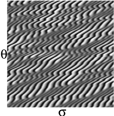
FIG. 1.: Space-time representation of the $CO_{2}$ laser intensity for a delay $\tau_{0}=400\mu s$ and for $\tau_{1}>\tau_{0}$ chosen so as to optimize the coherence of the vertical structures.

The most direct approach to the investigation of the dynamics of an experimental system consists in analysing the time record of a suitable observable. In the first part of this work [5], we discussed in detail the theoretical framework for the analysis of time-delayed feedback systems. In fact, it was necessary to develop a specific theory to reconstruct the equations of motion, since the high complexity of typical time-delayed feedback systems usually prevents the implementation of the standard embedding techniques[6, 7].

We are able to identify the deterministic structure underlying one such time series by adopting the ideas developed by Casdagli [8] for input–output systems. These are systems such as

$$\vec{x}_{n+1}=\vec{f}\left(\vec{x}_{n},\epsilon_{n}\right)\;,$$ (3)

where $\vec{x}_{n}\in{\mathbf{R}}^{d}$ is the state vector and $\epsilon_{n}$ is an additional time-dependent input. If a time series $\{y_{n}\}$ of some scalar observable $y(\vec{x})$ is available together with the (simultaneously recorded) input $\{\epsilon_{n}\}$, then Casdagli argued and more recently Stark et al. [9] have proven that the use of vectors of the form

$$\vec{v}_{n}=(y_{n},y_{n-1},\ldots,y_{n-m+1},\epsilon_{n},\epsilon_{n-1},\ldots,\epsilon_{n-m+1})$$ (4)

provide a proper embedding for $m>2d$. Such vectors unambiguously define the state of the system and in principle their knowledge uniquely determines the next observation $y_{n+1}$.

A discrete-time version of Eq. (1) has formally the same structure as an input-output system with the only difference that the input $\epsilon_{n}$ has to be replaced by the time-delayed value of the variable $x_{l}$ (see also [10, 11]). Therefore, a time series of $x_{l}$ allows to form vectors which are equivalent to those in Eq. (4). The same is possible also when the recorded variable does not coincide with the feedback one, although a higher-dimensional state space is required in this case (see Ref. [5]). More precisely, given the signal $x_{l}(t)$, we introduce the vectors

$$\vec{v}_{n}(m,\tau)=(y_{n},y_{n-1},\ldots,y_{n-m+1},y_{n-T},\ldots,y_{n-T-m+1}),$$ (5)

where $y_{n}=x_{l}(t=n\delta t)$ ($\delta t$ is the sampling time) and the integer $T$ corresponds to the physical time $\tau=T\delta t$. In Ref. [5], it has been shown that for $m>2d$ and $T=\tau_{0}/\delta t$, the knowledge of these vectors is (almost) sufficient to determine the future dynamics. In fact, some approximations arise because of the infinite-dimensional phase-space of the original continuous-time system that is replaced by a finite-dimensional space in the discrete-time representation. However, we have already seen in numerical simulations [5] and we shall confirm here by analysing experimental data that such approximations are harmless if the sampling time is sufficiently short.

A conceptually more satisfying reconstruction could be obtained by preserving the continuity of time, but this would be definitely less practical since the computation of derivatives from time-series data is a numerically unstable procedure that drastically increases any kind of noise.

The simplest convincing evidence that a given vector $\vec{v}_{n}(m,\tau)$ (for the rest of this work we will assume $\delta t=1$ and thus identify $T$ and $\tau$) provides a faitfhful reconstruction of the dynamics is through a good forecast of the next observation $y_{n+1}$. In practice, we introduce the following ansatz for the dynamics in the state space

$$y_{n+1}=h_{p}\left(\vec{v}_{n}(m,\tau)\right)\;,$$ (6)

where the function $h_{p}$ belongs to some class of parametrized functions. The unknown parameters $p$ are determined by minimizing the prediction error

$$\sigma_{m}=\sum_{n}(y_{n+1}-h_{p}\left(\vec{v}_{n}(m,\tau)\right))^{2}$$ (7)

with respect to the parameters $p$. A reasonable class of functions from the point of view of robustness, flexibility and numerical ease are local linear functions,

$$y_{n+1}=b_{n}+\vec{a}_{n}\vec{v}_{n}(m,\tau)\;,$$ (8)

where the parameters $\vec{a}_{n}$ and $b_{n}$ are determined for each individual $\vec{v}_{n}$ by fitting the behaviour in a suitable neighbourhood of $\vec{v}_{n}$ [12]. The resulting average forecast error (FCE) is thus computed as a function of $\tau$ for different embedding dimensions $m$. Its minima are used to determine the optimal choice of $m$ and $\tau$.

The representation of the dynamics by local linear maps allows most easily to compute the Lyapunov spectrum of the system, which is then approximated by $\tau+m$ exponents. It has been verified in many numerical simulations and there are good arguments showing that these are (approximations of) the largest $m+\tau$ exponents of the original system [13]. The implementation of this procedure will become definitely more transparent in Sec. III and IV where we discuss its application.

This paper is a case study on experimental data from a laser system to illustrate how far the investigation of a rather high dimensional dynamics can go when suitable methods are employed. Difficulties and limitations will be illustrated, but much more the overall power of the method will be proved.

In Sec. II, we describe the experimental set-up. In Secs. III and IV we study the low- and high-dimensional dynamics exhibited by the experiment for different delay times, while in Sec. V we present methods for the validation of the results. We will be able to obtain equations of motion that will be used for short time predictions, for the computation of the Lyapunov spectrum and for the generation of new time series, whose properties (such as the invariant measure) will be compared with the experimental data. Finally, we vary the time lag $\tau$ in the model equations obtained for a given delay time. This is to test the stability of the model that should be independent of the delay (as long as the equations of motion do not depend explicitely on $\tau$). The comparision of such numerically generated data with the experimental data obtained for the corresponding delay further confirm the validity of the reconstructed model. In summary, the following sections will demonstrate that the method proposed in [5] can be successfully employed in real experiments.

II The experimental setup

The experimental setup employs a single-mode CO₂ laser with an electro-optic feedback on the cavity losses (Fig. 2). The feedback consists in a signal proportional to the laser output intensity which, after a suitable delay and amplification, drives an intracavity electro-optic modulator. The intensity is detected with a fast Hg-Cd-Te photodiode and the delay line is realized using fast (2 MHz) and accurate (12 bits) A/D (analog-to-digital) and D/A converters allowing variations of the delay $\tau_{0}$ up to 130 ms with 0.5 $\mu$s resolution. The high-voltage amplifier adds to the delayed signal a continuous voltage level B which, once $\tau_{0}$ is fixed, acts as a control parameter. The overall error in the delay time is dominated by the delay line uncertainty, $\delta\tau_{0}=\pm 0.5\mu$s.

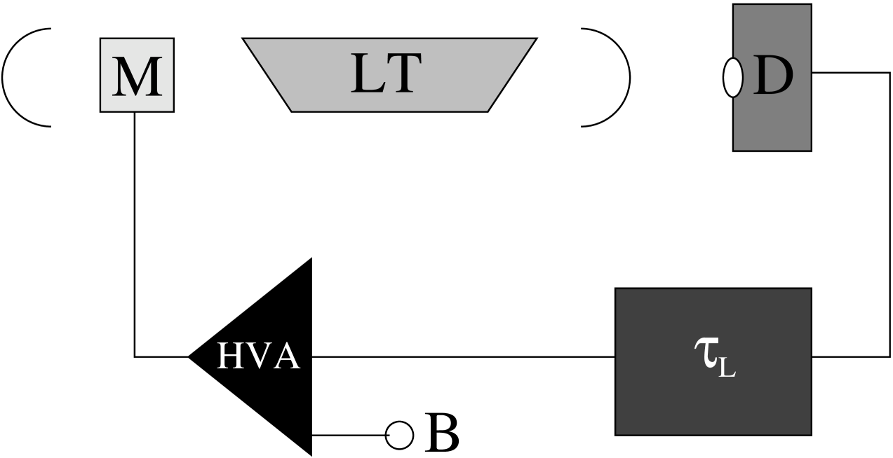
FIG. 2.: Scheme of the experimental setup: M, electro-optic modulator; LT, laser tube; D, detector; $\tau_{L}$, variable delay line; HVA, high voltage amplifier (amplification factor = 10000); B, bias voltage input.

The introduction of a delay $\tau_{0}$ in the feedback loop induces, upon increasing the bias B, a Hopf bifurcation with the frequency $f\approx 40.0$ kHz and the appearance of other incommensurate frequencies leading to the chaotic regime. Anyway, if $\tau_{0}$ is of the order of the characteristic period ($\sim$ 25 $\mu$s), the fractal dimension of the chaotic attractor remains between 2 and 3 [14, 15, 16]. Since the aim of the present work is to study the transition to a high dimensional chaotic regime characterized by more than one positive Lyapunov exponent, we have explored a delay range between $\tau_{0}=50\mu$s and $\tau_{0}=400\mu$s. For these $\tau_{0}$ values, the system shows the same qualitative behaviour. Superimposed to the Hopf oscillation, we observe a deep modulation paced by the inverse of the delay $\tau_{0}$, while the attractor becomes chaotic. A typical time sequence is shown in Fig. 2 (for B=250 V) together with the corresponding broad-band power spectrum. A further increase of B leads to a collapse of the attractor into a stable limit cycle.

FIG. 3.: (a) High dimensional time series of the $CO_{2}$-laser in the long delay regime, $\tau_{0}=400\mu$s. (b) Power spectrum of such a time series.

The chaotic time series analyzed in the next sections have been acquired by using a 12 bits A/D converter (LeCroy 6810) with sampling rate 1.0 $\mu$s and one million data memory.

The laser dynamics is influenced by “intrinsic” noise (dynamical noise) of the overall experimental setup. The latter is dominated by the noise of the electronic part of the feedback loop, which amount to approximately $3$ bits, i.e. about half a percent. This noise sets a lower bound for the prediction error computed later.

The simplest approach to model the dynamics of a single mode homogeneously broadened $CO_{2}$-laser is based on two rate equations for the laser intensity and the population inversion between the two relevant levels. However, this simple model is not adequate to fit data coming from experiments in the Q-switching regime, or in chaotic regimes obtained by sinusoidal modulation of the cavity losses, or with electro-optic feedback such as investigated in this paper.

A four-level molecular scheme, taking effectively into account the coupling between the resonant and some rotational levels provides a more accurate description of the laser dynamics. Nevertheless, the resulting model (a six-component DDE [17]) cannot be easily used to reproduce the behaviour of a $CO_{2}$-laser with electro-optical feedback because of the necessity of a fine tuning of the various parameters.

From the huge set of different measurements, we have selected three data sets we want to concentrate on in the rest of this paper. They mainly differ in the delay time, although other parameters of the laser were slightly modified too in order to keep the system in the same dynamical regime. The corresponding delays are $\tau_{0}=(50\pm 1)\mu s$, $\tau_{0}=(150\pm 1)\mu s$ and $\tau_{0}=(400\pm 1)\mu s$. The signal is sampled at times $t_{i}=i\delta t$ with the sampling time $\delta t=1.0\mu s$ in all three measurements. The laser intensity is measured with a 12-bit resolution (0-4095) and afterwards normalized such that $\langle y\rangle=0$, $\langle y^{2}\rangle=1$ in each individual time series. Each of the three data sets consists of $10^{6}$ points.

III The low dimensional case

We start the analysis of the laser system from the data set $\{y_{i}\}$ created with a sufficiently short delay time ($\tau_{0}=50$ $\mu$s) to ensure a low-dimensional dynamics. This has the advantage that we can cross-check our results with the outcome of standard embedding techniques.

The left panel of Fig. 4 shows the first 500 points of the time series. The delay time evidently represents a relevant scale of the system, since it corresponds to an approximate periodicity of the signal.

     

FIG. 4.: First 500 data of set with $\tau_{0}=50$ and the first 2000 points in a two dimensional delay representation.

The right panel shows a projection on the two-dimensional state space $(y(t-\tau_{0}),y(t))$ (here, we use the experimental knowledge of $\tau_{0}$; later, the delay time will be estimated from the time series). It gives a reasonable insight about the overall shape of the hypersurface on which the data lie. A characteristic signature of time-delayed systems is often found in the behaviour of the autocorrelation function and of the mutual information which exhibit a marked peak for a time difference slightly larger than the delay-time (see, for instance, [3]). Such revivals are clearly observable also in Fig. 5. In both cases, the first revival is situated at $\delta=58$, which is significantly larger than the delay time $\tau_{0}=50$. The reason is that the position of the peak does not depend only on the delay time, but also on the response of the system to the delayed feedback, so that one has to add an extra-delay due to the response time [18].

FIG. 5.: Autocorrelation (left panel) and time delayed mutual information (right panel).

Now, we discuss the implementation of the embedding technique described in [5]. In doing that, we consider that the delay $\tau_{0}$ is unknown and thus it is one of the quantities to be determined. We start computing the one-step prediction error $\sigma_{m}(\tau)$ (normalized to the standard deviation of the data) as a function of the time $\tau$ used in the reconstruction (see Eq. (5)) for $m=1,\ldots,5$. For a fair comparison of the results for different embedding dimensions, we ensured that the average neighborhood size employed in the local fits was the same (within small fluctuations) for all $m$. This means that we use the full data set of length $10^{6}$ only for $m=5$, while shorter segments are considered for smaller $m$. As a result, the systematic error due to the linear ansatz is the same for all dimensions. The results for $m=2,\ldots,5$ are reported in Fig. 6, where a clear minimum is observed in all cases: for $m=2$, the minimum is at $\tau=51\pm 1$, while for $m=3,4,5$, $\tau=50\pm 1$. Although the estimate of the delay time is in good agreement with our expectations, the forecast error is not very sensitive to variations in $\tau$ as, at most, it doubles when $\tau$ is grossly different from $\tau_{0}$. The only exception is the case $m=1$, not reported in the figure since it is approximately 50 times larger.

For $m\geq 2$ the minimal forecast error does never decrease below $\sigma\approx 2.3\cdot 10^{-3}$, which is mainly due to to the dynamical noise present in the experiment(see also Sec. II). In fact, the minimum error does not change by independently varying the size of the neighbourhood of the fit and the sampling time; therefore we can conclude that it can neither be attributed to modelling errors nor to the approximations inherent the map-ansatz (i.e. the projection of the infinite dimensional phase-space onto a finite-dimensional one). In Sec. IV, we shall find the same limitation on the FCE also for larger values of $\tau_{0}$.

FIG. 6.: Relative forecast error (multiplied by a factor of $10^{3}$) as a function of $\tau$ for embedding dimensions $m=2,\ldots,5$.

FIG. 7.: Lyapunov spectrum of the $\tau_{0}=50$ data set. The first exponent is estimated to be $\lambda_{1}\approx 1.8\ [1/{\rm ms}]$, while the second one is about a factor 10 smaller.

We now proceed with the determination of the Lyapunov spectrum by iterating the model equations. For this estimate we use again a variable number of points (depending on $m$) in order to ensure the same neighborhood size for the various embedding dimensions. The results are reported in Fig. 7 (Please note that the Lyapunov exponents are expressed in $1/{\rm ms}$ units rather than in the sampling frequency $1/\mu s$.). This analysis reveals only one positive Lyapunov exponent. One can also see that the first six exponents agree for all embedding dimensions, while irregular deviations are observed for the smaller ones. The reason for such deviations is not clear. It does not seem to be a systematic error, since there is no systematics observable by changing $m$. A possible explanation is a sensitivity of the very negative Lyapunov exponents to the details of the model which certainly change upon varying $m$ (because of the noise). In any case, the exponents involved in the determination of the Kaplan–Yorke dimension are not influenced and we find the following estimates for the dimension: $3.27$, $3.42$, $3.46$, $3.56$ for $m=2,3,4$ and $5$, respectively. By averaging these values, we can conclude that $D_{KY}=3.4\pm 0.1$. This value is small enough to allow us applying the methods of conventional nonlinear time-series analysis to validate the results. All numerical tools used here for this purpose are part of the TISEAN package [19, 20].

Since the marginally stable direction of flow data is unfavorable for the nonlinear analysis, we remove it. We construct a Poincaré map in the hyper-plane $\dot{y}=0$ by collecting all local maxima. The resulting data is shown in panel (a) of fig. 8. Although the noise level of the original flow data is fairly low, the Poincaré section is rather noisy. We thus apply the noise reduction algorithm presented in [21]. The result after 10 iterations (which turned out to be sufficient) is shown in panel (b) of Fig. 8.

FIG. 8.: Poincaré section of the flow data. Left panel before, right panel after applying a noise reduction scheme.

The figure shows that the noise reduction scheme allows resolving some singularities in the invariant measure of the data. Since the first negative Lyapunov exponent is close to zero (see Fig. 7), even the data of the Poincaré map look very much like flow data. Moreover, a clustering (a kind of phase locking) of the points is clearly visible: this is an artifact of the noise reduction which typically appears for flow data that are sampled almost in phase with the dominating frequency. The following results, however, are not significantly influenced by this clustering effect.

In Fig. 9, we show the behaviour of the correlation dimension [22]. The analysis was done for (standard) embedding dimensions $d_{E}=1,\ldots,10$. The dashed lines stem from the data before noise reduction (from bottom to top with increasing $d_{E}$). Due to the dominance of the noise, the only plateaus one sees are those corresponding to the embedding-space dimension, $d_{E}$. The solid lines in the figure show the behaviour after noise reduction. In this case, there is a nontrivial scaling behaviour on small length scales (smaller than $10^{-3}$). Though the estimates are still too fuzzy to derive a well defined dimension, the behaviour is in agreement with the Kaplan-Yorke dimension which corresponds to the horizontal line.

FIG. 9.: $D_{2}$ for the data in the Poincaré section. The solid lines show the result for the data after noise reduction, the dashed ones for the original data. The dashed horizontal line corresponds to the Lyapunov dimension obtained from the DM-model.

In the reconstructed phase space, one can obtain a model-free estimate of the maximal Lyapunov exponent by following the divergence of nearby segments of the trajectory. Also in this case (by implementing the procedure described in Ref. [23]), while we cannot draw a definite conclusion about the numerical value of the Lyapunov exponent, we can certainly say that the growth rate is consistent with the previous estimate of the Lyapunov spectrum.

The FCE is a local measure of the validity of a given model. However, as already seen in [5], a small FCE is a necessary condition for a global reproduction of the observed dynamics, but it is not at all sufficient. For this reason we have also decided to iterate the optimal models obtained for each value of $m$, starting from meaningful initial conditions (i.e. on the attractor). The ($m=1$)-dynamics leads to unbounded solutions. Accordingly, the hypothesis that a scalar model provides a convincing reconstruction of the dynamics can be rejected (notice that this conclusion was transparent already in view of the very large FCE found for $m=1$). For $m\geq 2$, the forward iterates of the local linear models remain bounded and their two-dimensional representations appear to be very similar to the experimental data (see Fig.4), so that we can conclude that the approximations implicit in the reconstruction with $m_{d}=2$ are small and harmless. In the second section, we mentioned that the minimal realistic model for a $CO_{2}$ laser with feedback involves 6 variables: the above result suggests that 4 of them can be, in a sense, adiabatically eliminated. This conclusion goes even beyond the application of the center manifold technique that allowed reducing the initial 6-dimensional model (in the case of short delay) to a 3-dimensional one [17].

Finally, we tried to model the dynamics by fitting autonomous models in the conventional embedding spaces. Although the attractor is fairly low dimensional, these models failed by either converging to fixed point solutions or diverging to infinity. Therefore, we can summarize the discussion on the low-dimensional chaotic dynamics by stating that the construction of a DM-model with $m\geq 2$ components is not only consistent with the application of standard methods of nonlinear time series analysis, but provides a more stable modellization. The superiority of the DM approach will become more transparent in the next section where we apply the method to high-dimensional signals, a case in which Takens-like embedding necessarily fails to give meaningful answers.

IV The high dimensional case

Past experience and the analogy with spatially extended systems indicate that large time-delays in the feedback loop enhance the complexity of the dynamics. In this section, we analyse the data sets obtained for $\tau_{0}=150$ and $\tau_{0}=400$, respectively. It will turn out that the attractor dimensions $D_{f}$ of these two series are indeed quite large, so that the standard embedding would fail due to the requirement $m>2D_{f}$. The aims are (i) to show that our ansatz allows us to model the data with reasonable accuracy and (ii) to estimate the minimal embedding dimension $m_{d}$ for a meaningful reconstruction. This gives an upper bound for the number $d$ of variables involved in the system [5].

As in the previous section, we employ the forecast error to identify the optimal delay time $\tau_{0}$. Again the length of the time series is varied from 20000 for $m=2$ to $10^{6}$ for $m=5$ to ensure a neighbourhood size almost independent of $m$ (approximately one percent of the attractor size).

FIG. 10.: Relative one-step prediction error (multiplied by $10^{3}$ in both panels) for the data sets with $\tau_{0}=150$ (left panel) and $\tau_{0}=400$ (right panel), respectively. The different curves correspond to different embedding dimensions.

The behaviour displayed by the FCE in Fig. 10 is qualitatively similar to that observed in the low–dimensional regime (reported in Fig. 6). At variance with the previous case, now there is a significant error reduction in passing from $m=2$ to $m=3$, but the minimum error does not further decrease by increasing $m$ beyond 3, meaning that the limit imposed by the noise level has been reached. Accordingly, this indicator does not allow drawing a definite conclusion about the relevance of additional degrees of freedom besides the first 3-ones. A further difference with the previous case is the larger value of the FCE for $\tau$ significantly different from $\tau_{0}$. In that region, the information contained in the second delayed window becomes increasingly negligible because of the decay of temporal correlations, so that the performance of our technique does not differ from that of the standard embedding approach for the same value of $m$. As here, at variance with the previous section, the attractor dimension is definitely larger than $m$ itself, larger FCE’s have to be expected for low-$m$ models.

The estimates of the delay times are reported in table I. Each value corresponds to the centre of the dip, while the error is the half-width of the dip. As in the low-dimensional case, we have investigated the peaks of the time delayed mutual information and of the autocorrelation. We find again an offset with respect to the known delay. For the data set corresponding to $\tau_{0}=150$, the peak lies at $\tau=157$ while for $\tau_{0}=400$ the peak is found at $\tau=407$. All such data together indicate that the offset is essentially independent of the delay, confirming that it is just the response time of the laser system to the feedback.

$\displaystyle\begin{array}[t]{|c|c|c|}\hline\cr m&\tau_{0}=150&\tau_{0}=400\\ \cline{1-3}\cr 2&152\pm 2&402\pm 2\\ 3&152\pm 2&402\pm 3\\ 4&151\pm 3&401\pm 4\\ 5&151\pm 3&401\pm 4\\ \hline\cr\end{array}$

TABLE I.: Estimates of the delay times for the $\tau_{0}=150$ and the $\tau_{0}=400$ data sets, respectively.

Together with the delay time, we now want to estimate $m_{d}$. Again, we require that a good model does not only yield good one-step forecasts but reproduces all the properties of the experimental data, when long trajectories are created by iterating the model itself. In other words we propose to compare global properties of the data sets [5]. Once we have verified that the trajectories do not escape to infinity under iteration of the model, we have determined the histograms of the data (i.e. the one-dimensional projection of the invariant measure) and the power spectra. Furthermore, we have investigated the convergence of the Lyapunov spectra as a function of $m$ and the behaviour of the cross–prediction errors between numerically generated time series and experimental data. For the sake of completeness, we have also investigated other indicators such as the mutual information, but we do not comment on the corresponding results as they simply confirm the overall scenario.

The comparison is performed as follows: for each embedding dimension we choose the optimal delay time from table I and accordingly generate an artificial trajectory which is used to compute the quantities to be compared with the corresponding ones obtained from the original data. If all of them (histograms, power spectra and Lyapunov exponents) agree for a given $m$, we can conclude that the $m$-value allows a faithful reconstruction. The smallest such $m$ is then defined to be $m_{d}$. Figures 11 and 12 show the results for the histograms and the power spectra, respectively.

FIG. 11.: One dimensional projection of the invariant measure of the original data and for modelled data in different embedding dimensions. Left panel (a): data set with $\tau_{0}=150$, right panel (b): data set with $\tau_{0}=400$. In both panels, the solid line corresponds to the original data, the dashed line to the fit for $m=3$, the dotted one to $m=4$ and the dashed–dotted one to $m=5$.

FIG. 12.: Power spectrum of the original data and for modelled data in different embedding dimensions. Left panel (a): data set with $\tau_{0}=150$, right panel (b): data set with $\tau_{0}=400$. The definition of the lines is the same as in fig. 11.

The histograms reported in Fig. 11 show a nonnegligible dependence on the embedding dimension (the curve for $m=2$ is not shown as it deviates even more strongly from the expected distribution). It is quite curious to see that while for $\tau_{0}=150$, simpler models ($m=3$, 4) give rise to a (spurious) peak around $y=-0.5$ which disappears upon further increasing $m$, the opposite is observed for $\tau_{0}=400$. We can understand this phenomenon by first noticing that $y\approx-0.5$ corresponds to an unstable fixed point of the dynamics (corresponding to the steady lasing state). Therefore, it turns out that a correct estimation of the stability of the fixed point is certainly crucial for a correct determination of the probability density in its surroundings. A posteriori, we can conclude that “underembedding” leads to a wrong estimation of the local stability.

The results for the power spectra are less clear. While for $\tau_{0}=400$, the relevant structures of the spectra are reproduced sufficiently well already for $m=3$, for $\tau_{0}=150$, differences are still observed by comparing the cases $m=3$ and $4$. Anyway, the relevant frequences are reproduced already for $m=3$, so that a clear conclusion about the appropriate $m_{d}$-value is quite hard to draw.

A more global test of the validity of a reconstructed model is through the computation of the cross–prediction error which is a measure of the “distance” between dynamical regimes. One might, for instance, be willing to compare different segments of the same time series to test the stationarity of the process as in Ref. [24]. In our context, the goal is to compare the original experimental signal $X=\{x_{n}\}$ with the computer generated trajectory $Y=\{y_{n}\}$, obtained by iterating the reconstructed model. More precisely, one uses the time series $Y$ as a data base to make a prediction $\tilde{x}_{n+1}(Y)$ for each possible value of $n$. This can be done by identifying the closest $Y$-points to each $X$ point in the $(2m)$-dimensional state-space and using them to construct a local linear model (see Ref. [5]). The average cross–forecast error is then defined as

$$\chi(X,Y)=\sqrt{\frac{\sum_{i=m}^{N}\left(\tilde{x}_{n}(Y)-x_{n}\right)^{2}}{(N-m)\sigma^{2}(X)}}\;,$$ (9)

where $\sigma^{2}(X)$ is the variance of the time series $X$. Notice that $\chi(X,X)$ reduces to the standard forecast error. Therefore, we expect $\chi(X,X)$ and $\chi(X,Y)$ to be approximately equal if $X$ and $Y$ follow the same dynamics.

$\displaystyle\begin{array}[t]{|c|c|c|}\hline\cr m&\tau_{0}=150&\tau_{0}=400\\ \cline{1-3}\cr\mbox{O}&5.0\cdot 10^{-2}&4.8\cdot 10^{-2}\\ \cline{1-3}\cr 2&11.9\cdot 10^{-2}&6.4\cdot 10^{-2}\\ 3&11.9\cdot 10^{-2}&6.0\cdot 10^{-2}\\ 4&10.3\cdot 10^{-2}&5.9\cdot 10^{-2}\\ 5&5.9\cdot 10^{-2}&6.1\cdot 10^{-2}\\ \hline\cr\end{array}$

TABLE II.: Estimates of the cross–prediction errors for the $\tau_{0}=150$ and the $\tau_{0}=400$ data sets, respectively. The row indicated by O is the usual prediction error using the original time series itself.

The results are shown in Tab. II. The first row shows the forecast error $\sigma(X,X)$ for both the $\tau_{0}=150$ and the $\tau_{0}=400$ data set. The forecasts are made with a zeroth order model (in five plus five dimensions) as described in Ref. [24, 5]. These results serve as references for the next lines. There, the cross–forecast errors are shown for data produced in the indicated embedding dimensions. Again the estimate of the error is done in five plus five dimensions. As for the spectra, we see differences between the two data sets. While for the $\tau_{0}=150$ data there is an improvement if $m$ is increased from $4$ to $5$, no such trend is visible for the $\tau_{0}=400$ data. There, the cross–forecast error is almost constant and comparably small already for $m=2$.

The convergence of the Lyapunov spectra as a function of $m$ is our last test. The resulting spectra are shown in Fig. 13. The left panel shows the first 30 exponents for $\tau_{0}=150$; in analogy with the previous analysis, we see that a convincing convergence is achieved only for $m\geq 5$ (the differences between the spectra for $m=5$ and $6$ concern the smaller Lyapunov exponents and are thus not dynamically relevant). The right panel of Fig. 13 shows the first 50 exponents for $\tau_{0}=400$. Again a faster convergence is observed as suggested from the cross-prediction error, although the Lyapunov spectrum appears to be a slightly more sensitive indicator as $m=4$ is the minimum embedding dimension for a convincing convergence.

FIG. 13.: Lyapunov spectra for the $\tau_{l}=150$ (panel a) and the $\tau_{0}=400$ (panel b) data sets. Note that the exponents are given in units of $1/ms$ and not in $1/\mu s$.

Taking into account all the results presented so far, it is rather difficult to draw a final conclusion about $m_{d}$. It is certainly true that $m=5$ is always sufficient to guarantee a good agreement with the experimental data, so that $m_{d}=5$ can be certainly considered as an upper bound to the minimal number of effective degrees of freedom to be used to construct the state-space. On the other hand, some properties are already recovered for $m=3$. This is confirmed by looking at Fig. 14, where the space–time representation of the $\tau_{0}=400$ data set (left panel) can be compared with the computer generated trajectory (right panel) obtained for $m=3$: no essential differences can be detected. While, it is not surprising that different indicators exhibit different sensitivity to modelling errors, it is somehow less understandable that the two data sets - corresponding to different delay times - give rise to different dependences on the embedding dimension. After a careful check of the original data, we have found that the time series with $\tau_{0}=150$ (the one exhibiting a slower convergence) is slightly corrupted by a noisy component at 50 Hz which evidently contributes to lowering the performance of our method. Anyway, in order to be on the safe side, in the remainder of the manuscript we shall always work with $m=5$.

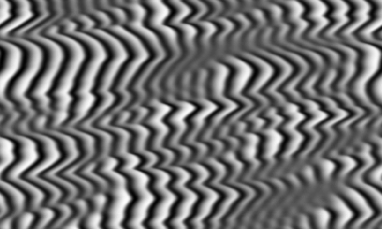
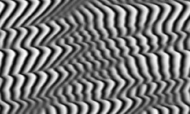
FIG. 14.: Space–time representation (as in fig. 1) of the $\tau_{0}=400$ data set. The left panel shows the original data, the right panel the data obtained by iterating a $m=3$ model.

The knowledge of the Lyapunov spectra allows to estimate both the fractal dimension $D_{KY}$ through the Kaplan-Yorke formula and the Kolmogorov-Sinai entropy $h_{KS}$ through the Pesin relation. From the results reported in Tab. III, we can see that the attractors are quite high dimensional: in both cases, $D_{KY}$ is larger than the dimension of our state space and, more importantly, is definitely beyond the limit for a successful application of the standard embedding approach.

Furthermore, our results on the attractor dimension in the various regimes provide the first experimental evidence that the dimension of a delayed system is proportional to the delay time. In fact, both in the low-dimensional chaotic regime examined in the previous section and in the two high-dimensional regimes studied here, we find approximately the same dimension density $d=D_{KY}/\tau_{0}\approx(64\pm 5)ms^{-1}$. This means that the addition of $(16\pm 1)\mu s$ to the delay line contributes to increasing the dimension by one unit. The extensivity of the fractal dimension, first noticed in [14] when studying the Mackey-Glass model, can be understood on the basis of the analogy with spatially extended systems which allows interpreting the delay as a “spatial” size of a suitable one-dimensional system [4].

$\displaystyle\begin{array}[]{|c|c|c|c|c|c|}\cline{1-6}\cr\tau_{0}&N&\lambda_{\rm max}$[1/{\rm ms}]$&D_{KY}&h_{\rm KS}$[1/{\rm ms}]$&D_{KY}/\tau_{0}$[1/{\rm ms}]$\\ \cline{1-6}\cr\cline{1-6}\cr 50&1&2.5&3.4&2.5&68\\ \cline{1-6}\cr 150&4&1.4&10.2&3.3&68\\ \cline{1-6}\cr 400&11&0.55&23.8&3.0&59\\ \cline{1-6}\cr\end{array}$

TABLE III.: Results exploring the Lyapunov spectra. $N$ is the number of positive Lyapunov exponents, $\lambda_{\rm max}$ the maximal exponent, $D_{KY}$ the Kaplan–Yorke dimension and $h_{\rm KS}$ the Kolmogorov-Sinai.

In contrast to the fractal dimension that is an extensive quantity, the dynamical entropy $h_{KS}$ of delay feedback systems turns out to be independent of the delay. The results reported in Tab. III clearly confirm this expectation. The reason for such a difference with truly extended systems (where the dynamical entropy too is extensive) can be traced back to the units of the “time” variable $\theta$ that have to be used for a meaningful space-time representation of delayed systems. As seen in Eq. (2), $\theta$ is essentially equal to the actual time except for a multiplicative factor equal to the delay time $\tau$ (for this discussion, the possible difference between $\tau_{0}$ and $\tau_{1}$ is immaterial). Accordingly, a dynamical entropy measured in ${\theta}^{-1}$ units has to be multiplied by $\tau$ and thus acquires an “extensive” character as expected for a spatially extended system.

The extensive character of the dimension and the intensive nature of the dynamical entropy both follow from a general property of the Lyapunov spectrum that is invariant (in the limit of long delays) under the simultaneous rescaling of the Lyapunov exponents by a factor $\tau$ and of the exponent’s index by $1/\tau$ [25]. Accordingly, the two spectra reported in Fig. 13 should collapse onto the same curve. This is indeed confirmed by Fig. 15, which at the same time confirms the correctness of the two-window embedding technique and provides experimental evidence for the scaling behaviour of the Lyapunov spectrum.

FIG. 15.: Rescaled Lyapunov spectra for the $\tau_{l}=150$ and the $\tau_{l}=400$ data sets. The exponents were calculated for $m=5$.

The spectrum obtained for $\tau_{0}=50$ does not overlap equally well. In complete analogy with space–time systems, this is certainly due to finite-“size” effects.

V Delay-time independence of the model

We started developing our theory under the assumption that we deal with delay differential equations such as in Eq. 1. The success of the two-window approach implies that the information contained in $\vec{v}_{n}$ is equivalent to that in $(\vec{x}(t),x_{l}(t-\tau_{0}))$ for $t=n\delta t$, provided that the correct value of $\tau=\tau_{0}$ is chosen in $\vec{v}_{n}$. Accordingly, there exists a delayed map $y_{n+1}=g(\vec{v}_{n})$ whose dynamics is equivalent to that stemming from the velocity field $f(\vec{x}(t),x_{l}(t-\tau_{0}))$. As a consequence, as long as the velocity field does not depend explicitly on $\tau$ (as it is the case in our experimental set-up), the same holds true for the mapping $g$.

The outstanding consequence is that the model constructed from a data set with some $\tau_{0}=\tau_{a}$ can be used to simulate the behaviour for a different delay $\tau_{0}=\tau_{b}$. The only problem comes from the lack of a global knowledge of $g$, which is inferred only in the region of the state-space visited by the input data. Therefore, the extension of the model to a different delay is possible only if, in the new regime, the dynamics does not leave the support of the invariant measure of the original one.

Iteration of a model constructed for $\tau_{0}=\tau_{a}$ with a different delay time $\tau_{b}$ can be executed in the following way. Let $\vec{v}_{i}(\tau_{a})$ be the vectors from the reference data set (our data base) and $\tilde{\vec{v}}_{i}(\tau_{b})$ the vectors to be produced. In order to forecast $\tilde{x}_{n+1}$ we determine $g$ in a small neighborhood of $\tilde{\vec{v}}_{n}(\tau_{b})$. This can be done by linearly approximating the set of all points $\vec{v}_{r}(\tau_{a})$ that are close to $\tilde{\vec{v}}_{n}(\tau_{b})$. Next, we use the fitted law to iterate $\tilde{\vec{v}}_{n}(\tau_{b})$. This is exactly the scheme of the cross-prediction described in the previous section, with the only difference that here the past window of $\tilde{\vec{v}}_{i}(\tau_{b})$ vectors differs from that of $\vec{v}_{i}(\tau_{a})$ ones.

More specifically, we have used the data set with $\tau_{a}=400$ to produce a trajectory simulating the behaviour for $\tau_{b}=150$. Since the dimension of the dynamics for $\tau_{a}$ is larger than that for $\tau_{b}$, we can expect that our artificial $\tau_{b}$-trajectory will not leave the region where we have to find $\tau_{a}$-neighbours (i.e., the support of the invariant measure for $\tau_{b}$ is a subset of that in the $\tau_{a}$ case). As an initial condition for the forecast, we used the first points of the $\tau_{a}$ data, so that we have to discard the initial transient.

FIG. 16.: First 1000 points of a trajectory with delay $\tau_{b}=150$ produced by using the data from the $\tau_{a}=400$ data set (panel a) and the original data from the $\tau_{0}=150$ data set (panel b).

Figure 16 shows 1000 points of the trajectory produced by the above described procedure. The main visible feature is a long periodicity approximately equal to $150\mu s$ , which matches the delay time $\tau_{b}$. Much more we cannot learn from this figure. In order to perform a more quantitative comparison we have looked at statistical properties of the data set. The left panel of fig. 17 shows the scalar distribution of the data.

FIG. 17.: Comparison of the invariant measure (more precisely the scalar distribution) (panel a) and the power spectrum (panel b) of the original data with $\tau_{b}=150$ (dashed line) and the data produced by iterating the $\tau_{a}=400$ model with $\tau_{b}=150$ (solid line).

The two lines shown in the plot are the distributions estimated from the computer generated (solid line) and from the original (dashed line) trajectory with $\tau_{b}$. The agreement is certainly comparable with that one guaranteed by the model constructed directly from the experimental data for $\tau_{b}$ (including the absence of a peak around $y=-0.5$). A similar conclusion can be drawn by looking at the power spectra in the right panel of the figures. In particular, the various peaks that are absent in the original dynamics at $\tau_{a}$ are located in the correct positions. The most significant deviations are found in the low-frequency region that is anyhow the most critical one as it can be observed in Fig.12.

As a last check we have computed the Lyapunov spectrum which agrees all the way down to the smallest exponents (see Fig. 18). Such a beautiful agreement must, however, be interpreted as a proof of the stability of the method (as we are comparing models obtained for two different delay times) rather than an indication of the correctness of the whole spectrum.

FIG. 18.: Similar to fig. 17, but for the Lyapunov spectra of both data sets.

We also tried to apply the same procedure to generate a trajectory with $\tau_{0}=50$. Unfortunately, all attempts have converged to a periodic orbit. In our opinion, the reason is the retuning of the bias voltage B in the experiment when switching from $\tau_{0}=50\mu s$ to $\tau_{0}=150\mu s$. In the low-dimensional case, several periodic windows can be detected in chaotic regions. Thus, a small change in a control parameter is likely to induce a transition either from chaotic to periodic behaviour or vice versa.

VI Conclusions

We have analysed the behaviour of a CO₂ laser with a time-delay feedback with a new embedding technique, designed to treat this class of systems. For a short delay-time, where the dynamics is low-dimensional, we have been able to check our methodology by comparing its results with those of well established methods from nonlinear time series analysis. Already in that case, the approach proved to be superior, allowing to construct a globally stable model. In the case of high-dimensional dynamics (longer delays) we have been able to model the system in a state-space of dimension significantly smaller than that of the attractor. We could show that the minimal embedding dimension needed to reproduce all relevant features is $m_{d}=5$, indicating that the active degrees of freedom of the laser are bounded between 2 and 5.

Furthermore, we have provided the first experimental evidence of the scaling behaviour of the Lyapunov spectra with the delay time. Accordingly, we have found that the dimension density is such that an additional active degree of freedom is created when the delay time is increased by 16 $\mu s$. Moreover, we have been able to confirm that the the dynamical entropy does not increase with the delay time.

Finally, we want to stress that with the identification of a model in the maximally chaotic regime (i.e. for sufficiently large delay) one could, in principle, study the whole bifurcation scenario of a delayed feedback system, upon changing the delay time. One could, for example, study the transition from standard chaos (one single positive Lyapunov exponent) to hyperchaos (more than one positive Lyapunov exponent) and compare with the experimental data. This interesting perspective is left to future investigations.

M.J.B. is supported by a Marie-Curie-Fellowship of the EU with the contract number: ERBFMBICT972305.; R. H. is partly supported by the EU with contract number: ERBFMRXCT96.0010 and wants to thank the colleagues at INOA for their kind hospitality. Support from the EU project PSS 1043 is also acknowledged.

REFERENCES

- [1] M. C. Mackey and L. Glass, Science 197, 287 (1977).
- [2] R. Lang and K. Kobayashi, IEEE J. of Quantum Electron. QE 16, 347 (1980).
- [3] F. T. Arecchi, G. Giacomelli, A. Lapucci, and R. Meucci, Phys. Rev. A 45, 4225 (1992).
- [4] G. Giacomelli and A. Politi, Phys. Rev. Lett. 76, 2686 (1996).
- [5] M. Bünner et al., Reconstruction of systems with delayed feedback: (I) Theory, European Physical J. D, submitted.
- [6] F. Takens, in Dynamical Systems and Turbulence (Warwick 1980), Vol. 898 of Lecture Notes in Mathematics, edited by D. A. Rand and L.-S. Young (Springer-Verlag, Berlin, 1980), pp. 366–381.
- [7] T. Sauer, J. A. Yorke, and M. Casdagli, J. Stat. Phys. 65, 579 (1991).
- [8] M. Casdagli, in Nonlinear Modeling and Forecasting, SFI Studies in the Sciences of Complexity (Addison-Wesley, Reading, 1992).
- [9] J. Stark, D. Broomhead, M. Davies, and J. Huke, Nonlinear Analysis, Methods & Applications 30, 5303 (1997).
- [10] R. Hegger, M. Bünner, H. Kantz, and A. Giaquinta, Phys. Rev. Lett. 211, 345 (1998).
- [11] M. J. Bünner, T. Meyer, A. Kittel, and J. Parisi, Phys. Rev. E 56, 5083 (1997).
- [12] J. Farmer and J. Sidorowich, Phys. Rev. Lett. 59, 845 (1987).
- [13] R. Hegger, Phys. Rev. E 60, 1563 (1999).
- [14] J. D. Farmer, Physica D 4, 366 (1982).
- [15] B. Dorizzi et al., Phys. Rev. A 35, 328 (1987).
- [16] G. Giacomelli, A. Lapucci, and R. Meucci, Phys. Rev. A 43, 4997 (1991).
- [17] A. Varone, A. Politi, and M. Ciofini, Phys. Rev. A 52, 3176 (1995).
- [18] G. Giacomelli, R. Hegger, A. Politi, and M. Vassalli, chao-dyn/9911025.
- [19] R. Hegger, H. Kantz, and T. Schreiber, CHAOS 9, 413 (1999).
- [20] R. Hegger, H. Kantz, and T. Schreiber, The Tisean Software Package, http://www.mpipks-dresden.mpg.de/tisean.
- [21] P. Grassberger et al., CHAOS 3, 127 (1993).
- [22] P. Grassberger and I. Procaccia, Phys. Rev. Lett. 50, 346 (1983).
- [23] H. Kantz, Phys. Lett. A 185, 77 (1994).
- [24] T. Schreiber, Phys. Rev. Lett. 78, 843 (1997).
- [25] G. Giacomelli, S. Lepri, and A. Politi, Phys. Rev. E 51, 3131 (1995).