SOGANG-ND 78/99
Phase Synchronization with Type-II Intermittency in Chaotic Oscillators

Abstract

We study the phase synchronization (PS) with type-II intermittency showing $\pm 2\pi$ irregular phase jumping behavior before the PS transition occurs in a system of two coupled hyperchaotic Rössler oscillators. The behavior is understood as a stochastic hopping of an overdamped particle in a potential which has $2\pi$-periodic minima. We characterize it as type-II intermittency with external noise through the return map analysis. In $\epsilon_{t}<\epsilon<\epsilon_{c}$ (where $\epsilon_{t}$ is the bifurcation point of type-II intermittency and $\epsilon_{c}$ is the PS transition point in coupling strength parameter space), the average length of the time interval between two successive jumps follows $\langle l\rangle\sim\exp(\mid\!\epsilon_{t}-\epsilon\!\mid^{2})$, which agrees well with the scaling law obtained from the Fokker-Planck equation.

Synchronization is one of the basic phenomena ubiquitously found in physical, chemical, biological and physiological systems. In the classical sense, synchronization of periodic self-sustained oscillators is usually defined as locking of the phases, $n\theta_{1}-m\theta_{2}=const$, due to weak interaction while the amplitudes can be quite different. This phenomenon has been quite well studied and has witnessed a lot of practical applications in various engineering fields [2].

Recently, the notion of synchronization has been extended to coupled chaotic oscillators (i.e., individual oscillators are chaotic without coupling). One of the remarkable developments is the observation of phase synchronization (PS) phenomenon in a system of two mutually coupled nonidentical self-sustained chaotic oscillators [3, 4]. The phenomenon is analogous to synchronization of periodic oscillators where only the phase locking is a matter of importance. Above a critical strength of coupling, suitably defined phases of two chaotic oscillators lock each other and synchronize, while their amplitudes remain chaotic and uncorrelated with each other. Also it was found that the phase difference $\phi$ between two oscillators increases with an intermittent sequence of $2\pi$ jumps before the PS transition occurs. It means that phase slips occur from time to time and the phase difference changes by $2\pi$ during a rather small interval of time.

The intermittent behavior and its scaling properties near the PS transition in a coupled Rössler system was studied by several authors [5, 6]. They provided an explanation for the phase jumps by reducing the original system into a simplified model describing an overdamped particle sliding in a “noisy wash-board potential”. Also by studying the scaling rules of the jumping behavior, they found that the phenomenon is related with type-I intermittency [8] in the presence of noise [5, 6]. So far, this has been known to be the only route to the PS transition in two coupled self-sustained chaotic oscillators, while nothing forbids other types of intermittency to exist.

In this paper, we report another route to PS transition exhibiting $\pm~{}2\pi$ jumps, which is characterized by the type-II intermittency with external noise. We consider the following two coupled hyperchaotic Rössler oscillators (HRO’s),

$$\stackrel{{\scriptstyle.}}{{x}}_{1,2} = -\Omega_{1,2}{y}_{1,2}-z_{1,2}+\epsilon({x}_{2,1}-{x}_{1,2}),$$ (1)

$$\stackrel{{\scriptstyle.}}{{y}}_{1,2} = \Omega_{1,2}{x}_{1,2}+0.25{y}_{1,2}+{w}_{1,2},$$ (2)

$$\stackrel{{\scriptstyle.}}{{z}}_{1,2} = 3.0+{x}_{1,2}{z}_{1,2},$$ (3)

$$\stackrel{{\scriptstyle.}}{{w}}_{1,2} = -0.5{z}_{1,2}+0.05{w}_{1,2}+\epsilon({w}_{2,1}-{w}_{1,2}),$$ (4)

where two variables $x$ and $w$ are coupled and the subscripts 1 and 2 refer to each of the oscillators. Here $\Omega_{1,2}=1.0\pm\Delta\Omega/2$  is the overall frequency of each chaotic oscillator, and $\epsilon$ is the coupling strength.

To observe PS we must define a suitable phase related to this system. Since the phase portrait of a hyperchaotic Rössler oscillator in the $x$-$y$ plane explicitly shows a rotational trajectory around a center, $(x_{0},y_{0})$ as shown in Fig. 1, the phase can be defined in relation with this rotation, i.e., $x_{1,2}$ and $y_{1,2}$ are transformed into polar variables $A_{1,2}$ and $\theta_{1,2}$ around the center of the rotation where $A_{1,2}=\sqrt{(x_{1,2}-x_{0})^{2}+(y_{1,2}-y_{0})^{2}}$ and $\theta_{1,2}=\tan^{-1}\left(\frac{y_{1,2}-y_{0}}{x_{1,2}-x_{0}}\right)$. With these variables, Eq. (1) can be rewritten as follows:

$$\stackrel{{\scriptstyle.}}{{A}}_{1,2} = 0.25A_{1,2}\sin^{2}\theta_{1,2}-z_{1,2}\cos\theta_{1,2}+\tilde{w}_{1,2}\sin\theta_{1,2}$$ (5)

$$+ \epsilon(A_{2,1}\cos\theta_{2,1}\cos\theta_{1,2}-A_{1,2}\cos^{2}\theta_{2,1}),$$ (6)

$$\stackrel{{\scriptstyle.}}{{\theta}}_{1,2} = \Omega_{1,2}+0.25\sin\theta_{1,2}\cos\theta_{1,2}$$ (7)

$$+ \frac{z_{1,2}}{A_{1,2}}\sin\theta_{1,2}+\frac{\tilde{w}_{1,2}}{A_{1,2}}\cos\theta_{1,2}$$ (8)

$$- \epsilon\left(\frac{A_{2,1}}{A_{1,2}}\cos\theta_{2,1}-\cos\theta_{1,2}\right)\sin\theta_{1,2},$$ (9)

$$\stackrel{{\scriptstyle.}}{{z}}_{1,2} = 3.0+({A}_{1,2}\cos\theta_{1,2}+x_{0}){z}_{1,2},$$ (10)

$$\stackrel{{\scriptstyle.}}{{w}}_{1,2} = -0.5{z}_{1,2}+0.05{w}_{1,2}+\epsilon({w}_{2,1}-{w}_{1,2}).$$ (11)

where $\tilde{w}_{1,2}$ is a shorthand for $w_{1,2}+x_{0}\Omega_{1,2}$ and $x_{0}=-16.0$ and $y_{0}=0.0$ are used. By solving Eq. (1) or (2) numerically, the phase difference ($\phi=\theta_{1}-\theta_{2}$) of the two oscillators is obtained as shown in Fig. 2. Note that the onset of PS occurs near $\epsilon_{c}=0.18$ [7]. Before the onset of PS, the smaller the coupling is the more frequently $2\pi$ jumps occur like the case of the Rössler system. But in our system, the phase difference jumps by $2\pi$ upwards or downwards irregularly as shown in Fig. 2, while in the Rössler case it jumps only upwards monotonously. In this respect, our system should be distinguished from the Rössler system qualitatively [3, 5, 6].

Here, we are interested in this new type of phase jumping behavior and would like to uncover the basic structure behind it. For this purpose, the following equation for the phase difference $\phi$ is obtained from Eq. (2):

$$\frac{d\phi}{dt} = \Delta\Omega+(0.25+\epsilon)(\sin\theta_{1}\cos\theta_{1}-\sin\theta_{2}\cos\theta_{2})$$ (12)

$$+ \frac{z_{1}}{A_{1}}\sin\theta_{1}-\frac{z_{2}}{A_{2}}\sin\theta_{2}+\frac{\tilde{w}_{1}}{A_{1}}\cos\theta_{1}-\frac{\tilde{w}_{2}}{A_{2}}\cos\theta_{2}$$ (13)

$$- \epsilon\left(\frac{A_{2}}{A_{1}}\sin\theta_{1}\cos\theta_{2}-\frac{A_{1}}{A_{2}}\cos\theta_{1}\sin\theta_{2}\right).$$ (14)

The r.h.s. of Eq. (3) can be rewritten in terms of $\phi$ by grouping relevant terms, and then we obtain the following phase equation similar to that describing phase locking of periodic oscillators in the presence of noise [3, 9, 10]:

$$\frac{d\phi}{dt} = \Delta\Omega+\alpha\sin\phi+\beta\sin\frac{\phi}{2}+\xi,$$ (15)

where

$$\alpha = (0.25+\epsilon)\cos(\theta_{1}+\theta_{2})-\frac{\epsilon}{2}\left(\frac{A_{2}}{A_{1}}+\frac{A_{1}}{A_{2}}\right),$$

$$\beta = 2\left\{\frac{z_{1}}{A_{1}}\cos\left(\frac{\theta_{1}+\theta_{2}}{2}\right)-\frac{\tilde{w}_{1}}{A_{1}}\sin\left(\frac{\theta_{1}+\theta_{2}}{2}\right)\right\},$$

$$\xi = \left(\frac{z_{1}}{A_{1}}-\frac{z_{2}}{A_{2}}\right)\sin\theta_{2}+\left(\frac{\tilde{w}_{1}}{A_{1}}-\frac{\tilde{w}_{2}}{A_{2}}\right)\cos\theta_{2}$$

$$- \frac{\epsilon}{2}\left(\frac{A_{2}}{A_{1}}-\frac{A_{1}}{A_{2}}\right)\sin(\theta_{1}+\theta_{2}).$$

Note that there are two time scales, i.e., the fast one, $2\pi/\Omega_{1,2}$, related with the frequency of each individual oscillator in Eq. (2), and the slow one, $2\pi/\Delta\Omega$, originating from the frequency mismatch in Eq. (3) which is the characteristic time of $\phi$ dynamics. Since $\alpha$ and $\beta$ and $\xi$ are fast fluctuating pieces compared with the time scale of $\phi$ variable, qualitative features of $\phi$ dynamics can be revealed after averaging $\alpha$ and $\beta$ over the slow time scale, while $\xi$ is left intact as an external noise in Eq. (4):

$$\frac{d\tilde{\phi}}{dt}=F(\tilde{\phi},\epsilon)+\xi,$$ (16)

where

$$F(\tilde{\phi},\epsilon)=\Delta\Omega+\langle\alpha\rangle\sin\tilde{\phi}+\langle\beta\rangle\sin\frac{\tilde{\phi}}{2}.$$ (17)

In Eq. (5) and (6), by $\tilde{\phi}$ we mean a new phase variable which simulates original $\phi$ dynamics. Here $\langle\alpha\rangle$, $\langle\beta\rangle$ represent averaged values for a long enough time interval which is order of $2\pi/\Delta\Omega$. This equation describes an overdamped particle moving in a potential under the influence of external noise $\xi$, where the potential $V(\tilde{\phi},\epsilon)$ is defined by $F(\tilde{\phi})=-\frac{dV(\tilde{\phi})}{d\tilde{\phi}}$ [5, 11]. This averaged potential is obtained by integrating the force $F(\tilde{\phi},\epsilon)$ with respect to $\tilde{\phi}$, i.e., $V(\tilde{\phi},\epsilon)=-\int^{\tilde{\phi}}F(\tilde{\phi}^{\prime},\epsilon)d\tilde{\phi}^{\prime}$ up to an arbitrary integration constant:

$$V(\tilde{\phi},\epsilon)=-\Delta\Omega\tilde{\phi}+\langle\alpha\rangle\cos\tilde{\phi}+2\langle\beta\rangle\cos\frac{\tilde{\phi}}{2}.$$ (18)

Figure 3 (a), (b), and (c) show time series of $\phi$ at $\epsilon=0.16$, the corresponding force $F$, and the potential $V$ respectively. As shown in Fig. 3 (c), the existence of $2\pi$-periodic minima is the main feature of the potential related with the phase jumping dynamics. Note that the overall slope of this potential is negligible due to the small constant force term $\Delta\Omega$, so that the “wash-board potential” picture [5] is not applicable to studying the bifurcation related with the intermittency in this system. With this potential structure, however, we can qualitatively explain the phase jumping dynamics as a hopping of an overdamped particle between $2\pi$-periodic minima in the potential through the stochastic process driven by the external noisy force $\xi$. In Fig. 3 (c), when a particle is in a potential well, it can jump randomly to the nearest neighboring potential wells since the barrier heights of both sides of the well are similar. When the well is not deep, the particle resides there for a short time interval, but it resides there longer when the well is deep. This behavior can be easily observed in the time series of $\phi$.

To determine the type of intermittency explicitly, we obtain the return map of $\phi$ from the original Eq. (2) by finding $\phi_{n}$ at every $2\pi$ rotation of phase $\theta_{1}$. Figure 4 (a) shows a schematic relation among force, potential, and the corresponding return map. In Fig. 4 (b), the return map shows many cells separated by $2\pi$ corresponding to $2\pi$-periodic minima in the potential structure. The trajectory in the return map moves from one cell to the neighboring cells irregurally in accordance with $\pm 2\pi$ jumps. To see the structure more clearly, we obtain the return map of $\tilde{\phi}$ from the averaged Eq. (5) in one cell at every $2\pi$ rotation of phase $\theta_{1}$ when $\xi=0$. The solid curves in Fig. 4 (b), (c), and (d) are the results and they quite well follow the one obtained directly from the original system (2). This means that the averaged Eq. (5) properly describes the main features of $\pm 2\pi$ phase jumping dynamics. From the shape of the curves, it is clear that the return map is actually that of type-II intermittency [8, 12]. In Fig. 4 (c) the center is a stable fixed point which becomes unstable when the slope at this point equals $1.0$ at the bifurcation point $\epsilon_{t}=0.038$ as shown in Fig. 4 (d). The trajectory can escape from the center to the nearest neighboring stable fixed points located each at $\pm~{}2\pi$ distance away through the stochastic process. Therefore the scaling of the average laminar length of $\phi$ (here the laminar length is the time elapsed between two successive $\pm 2\pi$ jumps) is expected to follow that of type-II intermittency in the presence of external noise.

In order to verify the above conjecture, we compare the average laminar length scaling relation obtained numerically from Eq. (2) with the analytical result obtained from the Fokker-Planck equation (FPE). The local Poincaré map of type-II intermittency with external noise is described by the following difference equation [11, 12, 13, 14]:

$$x_{n+1}=(1+\epsilon)x_{n}+ax_{n}^{3}+\sqrt{2D}\xi_{n},$$ (19)

where $a$ is a positive arbitrary constant, and $D$ is the dispersion of Gaussian noise $\xi_{n}$. It is well known that the above map (8) can be approximated to the backward FPE in the long laminar region [15]:

$$\frac{\partial G(x,t)}{\partial t}=-V^{\prime}(x)\frac{\partial G(x,t)}{\partial x}+D\frac{\partial^{2}G(x,t)}{\partial^{2}x}$$ (20)

where $G(x,t)$ is the probability density of particle at $(x,t)$. The scaling relation for the average escaping time can be derived analytically from this FPE. According to the analytical estimation made in our recent work [16], the average laminar length scales as follows when $\epsilon_{t}<\epsilon$:

$$\langle l\rangle\sim\langle l\rangle_{0}\exp(\mid\!\epsilon_{t}-\epsilon\!\mid^{2}).$$ (21)

Now, we perform numerical simulation to obtain the scaling law of the average laminar length from Eq. (2) and the results are shown in Fig. 5. First we get the value of $y$-intercept, $\ln\langle l\rangle_{0}$, in Fig. 5 (a) to determine the scaling exponent by the linear regression. The slope of the regression line in Fig. 5 (b) is very close to 2.0 within $\pm~{}5~{}\%$ error, which agrees with the scaling exponent in Eq. (10). Therefore our conjecture based on the return map analysis is verified and strengthened by this remarkable agreement with the result obtained from the FPE. Also this agreement in turn justifies our averaging out the fast fluctuating factors $\alpha$ and $\beta$ in Eq. (5), which marginally contribute as multiplicative perturbations in phase jumping dynamics.

In conclusion, we have firstly found the type-II intermittency route to the PS transition in a system of two coupled self-sustained HRO’s. In this system, the phase difference between two oscillators exhibits apparently irregular $\pm~{}2\pi$ jumps near the onset of the PS transition. Furthermore, we have identified this novel behavior as type-II intermittency with external noise through the return map analysis and the FPE approach.

We thank Dr. S. Rim and D. U. Hwang for valuable discussions. This work was supported by the Project of Creative Research Initiatives, Korea Ministry of Science and Technology. Y.-J. Park acknowledges the support from the Korean Council for University Education for 1999 Domestic Faculty Exchange.

FIG. 1.: The phase portrait of one of two coupled HRO’s projected on the $x$-$y$ plane. Initial values for HRO’s 1 and 2 are $x_{1}(0)=-20.0$, $y_{1}(0)=z_{1}(0)=0.0$, $w_{1}(0)=15.0$ and $x_{2}(0)=-20.1$, $y_{2}(0)=z_{2}(0)=0.0$, $w_{2}(0)=15.1$ respectively. Eq. (1) is numerically solved by using a fourth-order Runge-Kutta method with the parameter mismatch $\Delta\Omega=0.001$, and the same values are used throughout this Letter.

FIG. 2.: Time series of phase difference $\phi$ in two coupled HRO’s for various values of (a) $\epsilon=0.16$, (b) $\epsilon=0.17$, and (c) $\epsilon=0.18$. $\pm~{}2\pi$ phase jumps are shown for the cases of (a) and (b), while for (c) the PS transition seems to be achieved for the observed time scale.

FIG. 3.: (a) Time series of phase jumping dynamics, (b) the time-averaged force $F(\phi)$, and (c) the potential $V(\phi)$ at $\epsilon=0.16$.

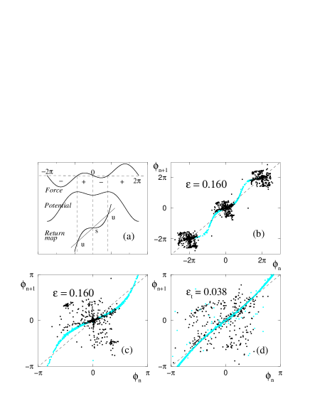
FIG. 4.: (a) schematic relation among force, potential, and return map; (b) return map (black dots) of original system (1) and return map (gray dots) from the averaged Eq. (4); (c) and (d) magnified return maps around one potential well with $\epsilon=0.16$ and $\epsilon_{t}=0.038$ respectively. Note that the tangent line at the center stable fixed point becomes tangential to the diagonal line in (d).

FIG. 5.: Scaling relation: average laminar length $\ln\langle l\rangle$ vs $\mid\!\epsilon_{t}-\epsilon\!\mid^{2}$ in (a) and $\ln(\ln\langle l\rangle-2.6)$ vs. $\ln\!\mid\!\epsilon_{t}-\epsilon\!\mid$ in (b). Note that the slope in (b) is approximately 2.0 within $\pm~{}5~{}\%$ error in agreement with the analytic estimation from the FPE.

REFERENCES

-
[1]
E-mail: chmkim@mail.paichai.ac.kr
- [2] I. I. Blekhman, Synchronization in Science and Technology (Nauka, Moscow, 1981 (in Russian)); English translation: (ASME Press, New York, 1988).
- [3] M. G. Rosenblum, A. S. Pikovsky and J. Kurths, Phys. Rev. Lett. 76, 1804 (1996); 78, 4193 (1997).
- [4] A. S. Pikovsky, M. G. Rosenblum, G. V. Osipov, M. Zaks and J. Kurths, Physica D 104, 219 (1997); M. G. Rosenblum, A. S. Pikovsky and J. Kurths, IEEE Trans. on Circuits and Systems-I, Vol.44, No.10, 874 (1997); E. J. Rosa, E. Ott, and M. H. Hess, Phys. Rev. Lett. 80, 1642 (1998); G. V. Osipov, A. S. Pikovsky, M. G. Rosenblum, and J. Kurths, Phys. Rev. E 55, 2353 (1997); A. S. Pikovsky, M. G. Rosenblum and J. Kurths, Europhys. Lett. 34, 165 (1996); O. Parlitz, L. Junge, W. Lanterborn, and L. Kocarev, Phys. Rev. E 54, 2115 (1996).
- [5] K. J. Lee, Y. Kwak and T. K. Lim, Phys. Rev. Lett. 81, 321 (1998).
- [6] W. H. Kye and C. M. Kim, to appear in Phys. Rev. E.
- [7] We cannot unambiguously determine the border of this transition. The transition to the synchronous state is always smeared and observed only as a tendency, or as a temporary event on some finite time intervals. According to Eq. (10), there doesn’t exist the onset point of PS because the average laminar length increases exponentially. But here the point is practically what can be observed in numerical simulation within the limit of computation time.
- [8] P. Manneville and Y. Pomeau, Physica (Amsterdam) 1D, 219 (1980); C. M. Kim, O. J. Kwon, E. K. Lee, and H. Y. Lee, Phys. Rev. Lett. 73, 525 (1994).
- [9] A. S. Pikovsky, Sov. J. Commun. Technol. Electron. 30, 85 (1985).
- [10] R. L. Stratonovich, Topics in the theory of Random Noise (Gordon and Breach, New York, 1963).
- [11] S. H. Strogatz, Nonliner Dynamics and Chaos (PERSEUS BOOKS, Reading, Massachusetts, 1994).
- [12] C. M. Kim, G. S. Yim, J. W. Ryu, and Y. J. Park, Phys. Rev. Lett. 80, 5317 (1998).
- [13] J. E. Hirsch, B. A. Heberman, and D. J. Scalapino, Phys. Rev. A 25, 391 (1982)
- [14] E. Ott, Chaos in Dynamical Systems (Cambridge University Press, 1994).
- [15] C. W. Gardiner, Handbook of Stochastic Methods (Springer-Verlag, 1985, 2nd ed.); H. Risken, The Fokker-Planck Equation (Springer-Verlag, 1996, 2nd ed.).
- [16] C. M. Kim, B. S. Yeom, W. H. Kye, and Y. J. Park, Characteristic Relations of Type-II and -III intermittency in the presence of noise, NRIC-preprint, (1999).