A New Feature in Some Quasi-discontinuous Systems

Many systems can display a very short, rapid changing stage (quasi-discontinuous region) inside a relatively very long and slowly changing process. A quantitative definition for the ”quasi-discontinuity” in these systems has been introduced. We have shown by a simplified model that extra-large Feigenbaum constants can be found inside some period-doubling cascades due to the quasi-discontinuity. As an example, this phenomenon has also been observed in Rose-Hindmash model describing neuron activities.
PACS: 05.45.+b

Recently, there has been considerable interest in piece-wise smooth systems (PWSSs). Such models usually describe systems displaying sudden, discontinuous changes, or jumping transitions after a long, gradually varying process. These systems may show some behaviors apparently different from those of the everywhere - differentiable systems (EDSs) [1-5]. In fact, the sudden changes in the above processes also need time. Therefore, such a process can be everywhere smooth if one describes it with a high enough resolution. Usually, in the largest part of the process, a quantity changes very slowly. It has a drastic changing only in one or several very small stages. We suggest to call the stage as a ”quasi-discontinuous region (QDR)” and shall define a ”quasi-discontinuity (QD)” inside it quantitatively. A system that can display QDR in its processes may be called a ”quasi-discontinuous system (QDS)”. Obviously, QDS is a much wider conception than PWSS and may serve as an intermediate between EDS and PWSS.

In order to show our basic idea and the first characteristic of QDS, we have constructed a model map as shown in Fig.1. The map reads:

$$f(x)=\left\{\begin{array}[]{ll}f_{1}(x)=k_{1}(x-x_{1})+y_{1}&x\in[0,x_{1}),\\ f_{2}(x)=A(x-x_{0})^{2}+y_{0}&x\in[x_{1},x_{3}),\\ f_{3}(x)=\sqrt{r^{2}-(x-o_{x})^{2}}+o_{y}&x\in[x_{3},x_{4}),\\ f_{4}(x)=k_{2}(x-x_{4})+y_{4}&x\in[x_{4},x_{5}),\\ f_{5}(x)=k_{3}(x-1)&x\in[x_{5},1].\end{array}\right.$$ (1)

As can be seen in Fig.1, the slope of $f_{1}$ branch is a unit. It is simulating the slowly changing part of the process. Branch $f_{4}$ is a linear line with a very large negative slope $k_{2}$. Branch $f_{3}$ is a small part of a circle introduced for a smooth connection of $f_{2}$ and $f_{4}$. The center of the circle locates at ($o_{x},o_{y}$), and its radius is $r$. Branches $f_{3}$ and $f_{4}$ can simulate the small drastic changing part. In Eqs. (1), $A$ is chosen as the control parameter. It is obvious that the fixed point at $P_{2}$ undergoes period-doubling bifurcation when $A$ changes inside a certain parameter range. $(x_{j},y_{j})$ denote the coordinates of points $P_{j}$ (j=0,…,5), respectively. They are determined by the conditions of smooth connections between neighboring branches. For certain function forms of $f_{2}$ and $f_{4}$, the circle of $f_{3}$ still may be very large or small. We define another parameter $\alpha$ to fix it. Therefore, $o_{x}$, $o_{y}$, $r$, $k$, and $(x_{j},y_{j})$ are all functions of $A$ and $\alpha$. Their explicit forms will not be shown in this short letter. The parameter ranges chosen for this study are $A\in[8.0,9.0]$ and $\alpha\in[0.99995,0.999997]$.

Now we will define QDR and QD in this model. According to the geometrical properties of Eqs. (1), one can obtain the following conclusions. When $\alpha=1$, $r=0$, the first order derivative of the map function is discontinuous at $x_{3}=x_{4}$. The second order derivative shows a singularity, that is, an infinitely large value here. When $\alpha\in(0,1)$, the branch $f_{3}$ has a finite length. The first order derivative of the map function is continuous at both $x_{3}$ and $x_{4}$. The second order derivative value between them is finite but trends toward infinite when $\alpha\rightarrow 1$. In this case, the maximum value of the second order derivative of the map function between $x_{3}$ and $x_{4}$ may be used to describe the ”quasi-discontinuity (QD)”. So we shall define QD as

$$\kappa=max{|\frac{d^{2}f}{dx^{2}}|_{x_{0}},x_{0}\in{[x_{3},x_{4}]}},$$ (2)

and define QDR as

$$\Delta=|x(2)-x(1)|,$$ (3)

where $x(2)$ and $x(1)$ are between $x_{3}$ and $x_{4}$, and satisfy

$$|\frac{df}{dx}|_{x(1)}=|\frac{df}{dx}|_{x(2)}=\frac{1}{\sqrt{2}}\max{|\frac{df}{dx}|}.$$

Acording to the definations (2) and (3), the QDR and QD for Eqs. (1) can be expressed as

$$x(1)=o_{x}-\frac{k_{2}r}{\sqrt{2+k_{2}^{2}}},\quad\quad x(2)=x_{4},$$ (4)

and

$$\kappa=\frac{-r^{2}}{[r^{2}-(x_{4}-o_{x})^{2}]^{3/2}},$$ (5)

respectively.

When $\alpha=1$ it is reasonable to observe one of the typical behaviors of PWSS. That is the interruption of a period - doubling bifurcation cascades by a type V intermittency [2,3].

When $\alpha$ is smaller than, but close to 1, there is a QDR between $x_{3}$ and $x_{4}$ instead of the non-differentiable point. The mapping is everywhere smooth, so the period-doubling bifurcation cascade should continue to the end. However, there is a drastic transition of the mapping function slope in a very small QDR that makes all further bifurcation points compressed into a relatively much shorter parameter distance. The Feigenbaum constants $\delta_{i}$ (i=3,4,5 or even more), influenced by the compression, should show some extraordinary values. That is exactly what we have observed. Table 1 shows the data about three cascades. In the table, $n$ indicate the sequence number of doubling, $\delta_{n}(i)$ $(i=1-3)$ are the Feigenbaum constants of the cascade $i$. The parameter values $\alpha(i)$ and the maximum value of the QD, $\kappa(i)$, for each cascade are indicated in the caption. In the table $\delta_{n_{0}}$ data are obtained from Ref. [6]. They are listed here for a comparison with the corresponding ones obtained in a typical everywhere smooth situation. As can be seen in table I, when $\kappa(i)$ is large, a lot of Feigenbaum constants, $\delta_{3}$, $\delta_{4}$, $\delta_{5}$, $\delta_{6}$ and $\delta_{7}$ are extraordinary. The further constants may be considered as ordinary, but they converge to the universal Feigenbaum number very slowly. When $\kappa(i)$ is smaller, only $\delta_{3}$, $\delta_{4}$ and $\delta_{5}$ are apparently extraordinary. The further constants converge much faster. When $\kappa(i)$ is very small, the whole Feigenbaum constant sequence is very close to the standard $\delta_{n_{0}}$ data. That may indicate a smooth transition from QDS to a EDS. Also, from these data one can believe that the extraordinary Feigenbaum constants in the period-doubling cascades are induced by QD of the system. Based on this understanding we suggest the use of the common extraordinary Feigenbaum constant $\delta_{j}(j=3,4)$ to signify this phenomenon. The relationship between $\kappa$, the QD, and the symbol of the phenomenon $\delta_{j}$ ($j=3,4$), have been computed. Figure 2 shows the result of function $\kappa-\delta_{j}$( Although $\kappa$ is dependent on both $\alpha$ and $A$, our numerical results demonstrate that $\kappa$ is not sensitive to the parameter $A$ at a given $\alpha$. Therefore, it is possible to choose the maxmum $\kappa$ to represent QD of a whole diagram. For example, for the bifurcation points $A_{n}(n=0,1,2,...,12)$, indicated in the second column of Table 1, the corresponding $\kappa$ are $220.9\times 10^{6}$, $208.2\times 10^{6}$, $205.6\times 10^{6}$, …, $205.0\times 10^{6}$, respectively. So we choose $220.9\times 10^{6}$ as the representative $\kappa$ of the bifurcation diagram). One can see that $\delta_{4}$ increases, but $\delta_{3}$ decreases when $\kappa$ becomes larger and larger.

It is important to find examples of this kind of interesting phenomenon in practical systems. We have done such a study in Rose-Hindmarsh (R-H) model. The model, which describes neuronal bursting [7], can be expressed by

$$\left\{\begin{array}[]{l}\frac{dx}{dt}=y-ax^{3}+bx^{2}+I-z,\\ \frac{dy}{dt}=c-dx^{2}-y,\\ \frac{dz}{dt}=r[s(x-x^{*})-z],\end{array}\right.$$ (6)

where $x$ is the electrical potential of the biology membrane, $y$ is the recovering variable, $z$ is the adjusting current, $a,b,c,d,s$ and $x^{*}$ are constants, $r$ and $I$ are chosen as the control parameters. We shall take $a=1,b=3,c=1,d=5,x^{*}=1.6,s=4$ for this study. Fig.3 shows the ${\rm Poincar\grave{e}}$ map of a strange attractor observed when $I=2.9,r=0.00433$ (Here the ${\rm Poincar\grave{e}}$ section is defined as the coordinate value of z axis at the maximum in x direction of the trajectory. We have also tested some different definitions of ${\rm Poincar\grave{e}}$ section, the results have shown that all of them are qualitatively the same as each other). It is clear that the iterations in the region $[z_{1},z_{2}]$ change very rapidly. Therefore, we call this region as a QDR.

Table 2 shows the critical bifurcation parameter values and the corresponding Feigenbaum constants for a period-doubling bifurcation cascade. One can see that $\delta_{1}$ and $\delta_{2}$ are larger than ordinary values. As our computation has confirmed, that means an interruption of the cascade by a collision of the periodic orbit with the QDR when the first time period-doubling finished.

For a comparison with the function $\kappa-\delta_{i}$ shown in Fig. 2, we have computed the bifurcation diagrams with $I=2.8,2.9,3.0,3.1,3.2,3.3,3.4$, and $r\in[0.1\times 10^{-2},4\times 10^{-2}]$. The results are shown in Fig. 4 (Here, we also choose the maxmum $\kappa$ to represent the quasi-discontinuouty of one bifurcation diagram). They are in a qualitative agreement with those in Fig. 2.

In conclusion, we have found some extraordinary Feigenbaum constants in some period-doubling bifurcation cascades in a constructive and a practical system. The mechanism of the phenomenon is that a periodic orbit near a critical point of bifurcation crosses a QDR in the system. This understanding may be important for the experimental scientists because very often they can measure only the first several Feigenbaum constants in a real experiment. After observing strange Feigenbaum constants, they can verify if their system is a QDS with the knowledge in this discussion. Moreover, our results also demonstrate that between typical PWSSs and EDSs there can be a type of transitive systems.

TABLE I.: The data for period-doubling bifurcation cascades in Eqs. (1) with $\alpha=0.9999970$ and $\kappa_{max}=220.9\times 10^{6}$ for cascade (1); $\alpha=0.9999196$ and $\kappa_{max}=8.2\times 10^{6}$ for cascade (2); $\alpha=0.9987537$ and $\kappa_{max}=0.5\times 10^{6}$ for cascade (3). The data are obtained by numerical method with a quadruple precision.

n	$\delta_{n}(1)$	$\delta_{n}(2)$	$\delta_{n}(3)$	$\delta_{n_{0}}$
1	4.626168416	4.626168416	4.626168416	4.744309468
2	4.638635250	4.638635250	5.965311262	4.674447827
3	8.823236594	9.982064249	7.746315906	4.670792250
4	16.553602405	11.112580986	4.756159889	4.669461648
5	1.619920263	3.966760226	4.705758197	4.669265809
6	4.147211067	4.411839476	4.674983020	4.669214270
7	5.173386810	4.526007508	4.670687838	4.669204451
8	4.765263421	4.709611842	4.669607200	4.669202201
9	4.757647408	4.671017586	4.669986034	4.669201737
10	4.687625667	4.677922775	4.669375410	4.669201636
11	4.701929236	4.703838840	4.699239861	4.669201614

TABLE II.: The data of the bifurcation critical parameter values and the corresponding Feigenbaum constants observed in system (6) with $I=2.8$.

n	$r_{n}\times 10^{-2}$	$\delta_{n}$
0	3.52000
1	1.55550	19.84344
2	1.45650	6.14905
3	1.44040	5.19350
4	1.43730	4.76981
5	1.43665

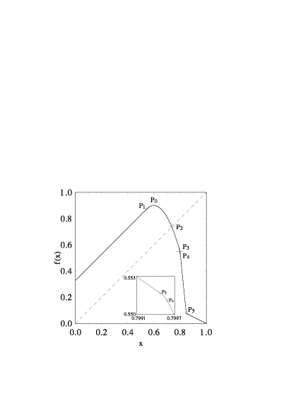
FIG. 1.: Function of Eqs. (1) when $A=8.75407,\alpha=0.998$. The inset is the enlargement area near $P_{3}$ and $P_{4}$.

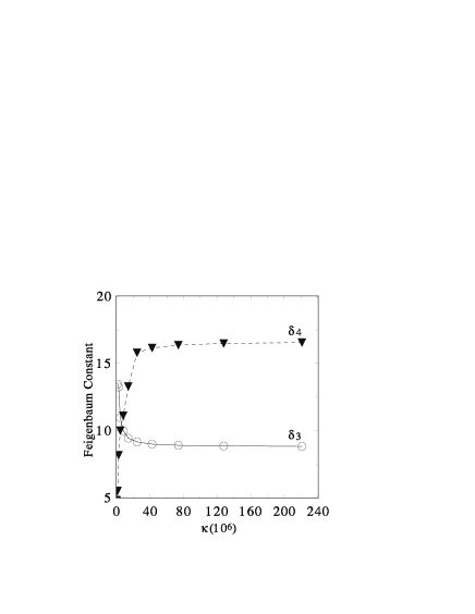
FIG. 2.: The function $\kappa-\delta_{i}$ for Eqs. (1) with the parameter value $\alpha\in[0.99966,0.999997]$.

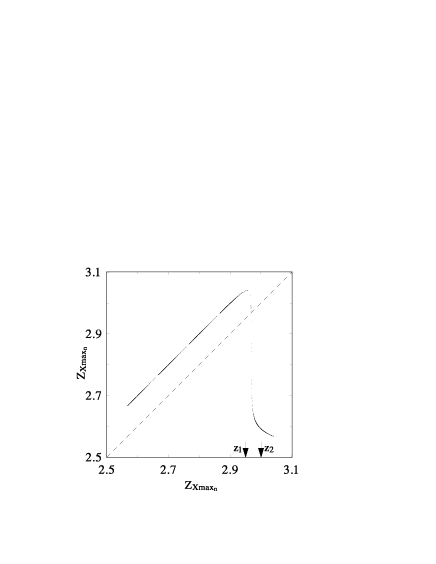
FIG. 3.: The ${\rm Poincar\grave{e}}$ map of R-H model. Here the range $[z_{1},z_{2}]$ schematically indicates the QDR, the real QDR calculated via Eq.(3) is too small to be clearly expressed.

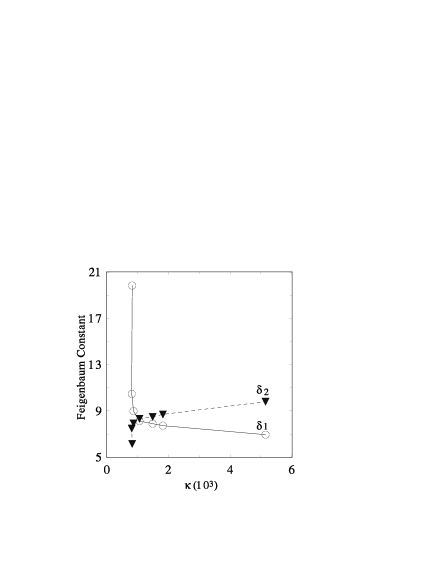
FIG. 4.: The function $\kappa-\delta_{i}$ for period-doubling bifurcation’s in R-H model.

REFERENCES

- [1] L. Glass, Chaos, 1 (1991) 13.
- [2] D.-R. He et al. Phys. Lett. A 171 (1992) 61.
- [3] C. Marriot and C. Delisle, Physica D 36 (1989) 198.
- [4] C. Wu, S. Qu, S. Wu and D.-R. He, Chin. Phys. Lett. 15 (1998) 246.
- [5] X. Ding, S. Wu, Y. Yin and D.-R. He, Chin. Phys. Lett. 16 (1999) 167.
- [6] M.J. Feigenbaum, J. Stat. Phys. 19 (1978) 158.
- [7] J. L. Hindmarsh and R. M. Rose, Nature(Landon), 296 (1982) 162.