Sensitive boundary condition dependence of noise-sustained structure

Abstract

Sensitive boundary condition dependence (BCD) is reported in a convectively unstable system with noise, where the amplitude of generated oscillatory dynamics in the downstream depends sensitively on the boundary value. This BCD is explained in terms of the manner in which the co-moving Lyapunov exponent (characterizing the convective instability) decreases from upstream to downstream. It is shown that a fractal BCD appears if the dynamics that represent the spatial change of the fixed point includes transient chaotic dynamics. By considering as an example a one-way-coupled map lattice, this theory for BCD is demonstrated.

Convective instability, which causes amplification of a disturbance along flow[1, 2], is generally important in open flow systems [2, 3]. If a system is convectively unstable (CU), a small disturbance at an upstream position is amplified and transmitted downstream. Due to this property, spatiotemporal structure with a large amplitude can be generated in the downstream by a tiny fluctuation in the upstream. Such structure is referred to as noise-sustained structure (NSS)[3].

Convective instability is quantitatively characterized by a co-moving Lyapunov exponent $\lambda_{v}$, i.e., the Lyapunov exponent observed in an inertial system moving with the velocity $v$ [4, 5]. If $\mathop{max}_{v}\lambda_{v}$ is positive for a given state, the state is convectively unstable. This condition is compared to that for linear instability, implies $\lambda_{0}>0$. Absolute stability (AS), which implies stability along any flow[1, 2], is guaranteed by the condition $\mathop{max}_{v}\lambda_{v}<0$. (With respect to an attractor, the co-moving Lyapunov exponent is used as an indicator of chaos: chaos with convective instability is characterized by the positivity of $\mathop{max}_{v}\lambda_{v}$. However, with respect to a state, it is generally used to characterize its stability.)

In a system with convective instability and noise, we have shown that the downstream dynamics depend on the boundary condition at the upstream. Such behavior exhibiting some threshold-type dependence on the boundary condition was identified and analyzed in connection with the change of the convective instability along the flow[6]. In the present letter, we demonstrate that sensitive BCD of the downstream dynamics can appear in a class of noisy open-flow systems, and we clarify the condition for this appearance.

In this letter we consider the simple case of a discrete system in one spatial dimension of the kind described above. As a simple example, we adopt a one-way coupled map lattice (OCML) [5, 7, 8, 9, 10, 11] with noise:

$$x_{n}^{i}=(1-\epsilon)f(x_{n-1}^{i})+\epsilon f(x_{n-1}^{i-1})+\eta_{n}^{i}.$$ (1)

Here $n$ is a discrete time step, $i$ is the index denoting elements ($i=1,2,,,,M=$ system size), and $\eta$ is a white noise satisfying $<<\eta_{n}^{i}\eta_{m}^{j}>>=\sigma^{2}\delta_{nm}\delta_{ij}$, with $<<...>>$ representing an ensemble average ($\sigma\ll 1$)[12]. A fixed boundary condition $x^{0}$ is adopted and the (sensitive) dependence of the downstream dynamics on $x^{0}$ is studied. The use of a CML here is just for convenience for illustration. The results and theory we present are straightforwardly adapted to the case of coupled ordinary differential equations (ODE).

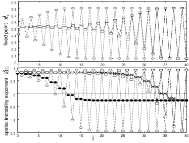
Figure 1: The patterns $x_{*}^{i}$ and $\lambda^{S}(i)$. The upper figure displays the fixed-point pattern $x_{*}^{i}$ in the absence of noise, while the lower figure displays the spatial pattern of $\lambda^{S}(i)$. Two sets of plots are overlaid for different values of the boundary, $x^{0}=0.52$ (solid line with $\Box$) and $0.60$ (dotted line with $\circ$). For the lower figure $\sum_{\ell=0}^{1}\lambda^{S}(i-\ell)/2$ ($\times$ for $x^{0}=0.52$, $\bullet$ for $0.60$) is also plotted. This difference reflects the difference in the downstream dynamics in the case with noise. For the boundary value for $x^{0}=0.60$ no oscillation is generated in the downstream (since the CU region is narrow, as discussed in the text), while oscillation is generated in the downstream for $x^{0}=0.52$, as shown in Fig.3. Here, $a=1.8,\epsilon=0.83$.

In the present case we choose the logistic map $f(x)=1-ax^{2}\ (-1<x<1)$. The parameters $a$ and $\epsilon$ are chosen so that in the noiseless case all elements are attracted to fixed points $x_{n}^{i}=x_{*}^{i}$ for any initial and boundary conditions [i.e., the fixed points (in time) are AS in the downstream]. This attraction to fixed points is realized in the strong coupling regime (see Ref.[9]). The values of the fixed points can depend on the lattice site number (i.e. can be functions of space), and set of points {$x_{*}^{i}$} form a spatially periodic pattern, as show in Fig.1. When noise is added, however, it can be amplified in the downstream to create oscillating motion (see Fig.2) if the upstream fixed points are convectively unstable [3].

Whether or not this noise-sustained structure is formed in the downstream depends on the boundary value $x_{0}$ and the noise strength. As a rough measure for the amplitude of the downstream oscillation, the root mean square (RMS) $\sqrt{<x_{n}^{i}-<x_{n}^{i}>>^{2}}$ is computed, where $<...>$ is the temporal average. As shown in Fig.3, the RMS has a threshold-type dependence on $x_{0}$. Such a BCD has been observed in a one-way coupled ODE[6]. The mechanism responsible for the sensitive BCD clarified in that study is universal and can be summarized as follows: A change in $x^{0}$ causes a change in the value of upstream fixed points $x_{*}^{i}$, which in turn causes a change in the degree of convective instability. Accordingly the downstream dynamics, generated through the spatial amplification of noise, can be different for different values of $x^{0}$.

In the present case this mechanism is quantitatively analyzed as follows: The spatial fixed points dynamics are described by the spatial recursive equation

$$\begin{array}[]{rcl}x_{*}^{i}&=&(1-\epsilon)f(x_{*}^{i})+\epsilon f(x_{*}^{i-1})\\ &=&\frac{-1+\sqrt{1+4a(1-\epsilon)(1-a\epsilon(x_{*}^{i-1})^{2})}}{2a(1-\epsilon)}\\ &\equiv&g(x_{*}^{i-1}),\end{array}$$ (2)

while the co-moving Lyapunov exponent $\lambda_{v}(i)$ of each fixed point $x_{*}^{i}$ [6, 10] is given by

$$\begin{array}[]{rcl}\lambda_{v}(i)&=&(1-\epsilon)\mbox{log}|f^{\prime}(x_{*}^{i})|+\epsilon\mbox{log}|f^{\prime}(x_{*}^{i-1})|\\ &&+\mbox{log}|\frac{1-\epsilon}{1-v}|+\mbox{log}|\frac{\epsilon(1-v)}{v(1-\epsilon)}|^{v}.\end{array}$$ (3)

A relevant quantity, characterizing the amplification of a disturbance per lattice site is given by the spatial instability exponent $\lambda^{S}(i)$ [13],

$$\lambda^{S}(i)=max_{v}\frac{\lambda_{v}(i)}{v}.$$ (4)

In Fig.1, $\lambda^{S}(i)$ is also plotted as a function of the lattice site number. For both the boundary values $x^{0}=0.52$ ($\Box$) and $x^{0}=0.60$ ($\circ$), convective instability exists in the upstream, as indicated by $\lambda^{S}(i)$. (Here the downstream pattern has spatial period 2, and $\lambda^{S}(i)$ also oscillates with this period. For this reason, $\sum_{\ell=0}^{1}\lambda^{S}(i-\ell)/2$, the average over the spatial period, is also plotted.) For $x^{0}=0.60$, $\lambda^{S}(i)$ (or the average over the spatial period) becomes negative at a smaller lattice site number than the case for $x^{0}=0.52$. In fact, as discussed below, this difference in the convergence rate of $\lambda^{S}(i)$ is relevant to the BCD of the downstream dynamics.

Since we have assumed that the fixed point pattern is AS in the downstream, the noise has to be amplified at a lattice point where the fixed point remains CU, in order for NSS to be formed. First, we estimate the lattice point $i_{u}$, defined as the site where the convective instability is lost; in other words, the site where the fixed point $x^{i}_{*}$ changes from CU to AS. Recall that the $x^{i}_{*}$ approach a periodic pattern in the downstream in the absence of noise. Denoting this spatial period by $L$, the lattice point $i_{u}$ is given by the point $i$ such that $\sum_{\ell=0}^{L-1}\lambda^{S}(i-\ell)/L$ is positive for $i<i_{u}$ and negative for $i\geq i_{u}$. As can be also expected by considering Figs.1 and Fig.3, $i_{u}$ is strongly correlated with the relaxation scale of the spatial map. If the convergence of the spatial map to its attractor is more rapid, $i_{u}$ is generally smaller. (See Fig.1: for example, $i_{u}=12$ for $x^{0}=0.60$ indicated by $\bullet$, while $i_{u}=36$ for $x^{0}=0.52$ indicated by $\times$.)

On the other hand, the scale $i_{g}$ required for the amplification of a tiny noise to $O(1)$ can be estimated by $\sigma\mbox{exp}(\sum^{i_{g}}_{i=1}\lambda^{S}(i))\sim 1.$ Then, the condition [6] for the formation of NSS is simply given by

$$i_{u}-i_{g}\geq 0.$$ (5)

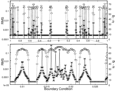
Figure 4: BCD of the RMS of $x^{200}$ ($\circ$) and $i_{u}-i_{g}$ ($\times$), with $\epsilon=0.9108$, spatial period = 4, and $\sigma=2\times 10^{-4}$. The lower figure is the blow-up of the upper figure.

In Fig.4, we have plotted $i_{u}-i_{g}$ and the RMS of downstream dynamics as function of the boundary value $x^{0}$. The numerical results clearly support the conclusion that the condition for NSS is given by $i_{u}-i_{g}\geq 0$. Although this condition concerns only the sign of $i_{u}-i_{g}$, the amplitude of the NSS is also highly correlated with the value of $i_{u}-i_{g}$, as shown in Fig.4. In the case of Fig.3, the downstream AS dynamics are of spatial period 2, where NSS appears around $x^{0}=0.52$ and $0.97$. The BCD here is simple, with just two regions allowing for NSS. For the case of spatial period 4, as shown in Fig.4, there are many undulation, and this BCD has a self-similar fine structure, to be shown as fractals (see the blow-up of Fig.4). The complexity of this self-similar structure of the BCD increases with the period, as shown in Fig.5 for the case of spatial period 16. With this self-similar structure, a small difference in the boundary value results in a large difference in the downstream dynamics.

We now discuss the origin of such sensitive BCD. As seen from Figs.4 and 5, this BCD is due to the complicated structure of the BCD of $i_{u}-i_{g}$. Here, $i_{g}$ has a rather smooth dependence on $x^{0}$, and the complicated structure is due mainly to $i_{u}$. In fact, there are (infinitely) many local maxima of $i_{u}$ considered as a function of $x^{0}$, in analogy to the plot of $i_{u}-i_{g}$ in Fig.4.

Recall that the scale $i_{u}$ is highly correlated with the duration of the transient process of the spatial map Eq.(2), i.e., the number of steps required for an orbit, generated by the map starting from $x^{0}$, to fall into a periodic attractor. When the period of the attractor of the map $g(x)$ is $L$, there are $L$ stable fixed points for the map $x\rightarrow g^{L}(x)$. Each stable fixed point corresponds to a different phase of the periodic attractor of the spatial map $g(x)$. For each value of the initial condition $x^{0}$ in the spatial map, the fixed point to which the $g^{L}(x)$ map is attracted [i.e., the phase of the cycle in the map $g(x)$] is different.

When multiple attractors coexist, it is often the case that the basin structure for each attractor is fractal [14]. This is true for $g^{L}(x)$, and here there can be infinitely many basin boundary points. For example, in Fig.6 we have plotted the basin boundary points in the spatial map. For the spatial period 2 case, there are 4 such points, as shown in Fig.6(a), while there are infinitely many points and the basin boundary is fractal for the case of spatial period 4 (or higher), as shown in Fig.6(b). Note that at unstable fixed points of $g^{L}(x)$, the phase of the attracted cycle slips. Successive preimages of such fixed points are nothing but the basin boundary of the map $g^{L}(x)$, with which fractal basin boundary is formed.

For each basin boundary point, the number of transient steps before the attraction of an orbit to an attractor diverges. Hence, $i_{u}$ takes a local maximum at each point. Accordingly, there are infinitely many local maxima of $i_{u}$, organized in a self-similar manner. Now, the sensitive dependence on $x^{0}$ is understood resulting from a fractal basin boundary in the spatial map. Since this formation of a fractal basin boundary is rather common in one-dimensional maps (with topological chaos), sensitive BCD is expected to be a general phenomenon. Here, it should be stressed that although the mechanism here is based on the fractal basin in the spatial map, the sensitive dependence is explained as a dependence on the boundary condition rather than the initial condition[15].

In conclusion, we have demonstrated the existence of a sensitive BCD in a system characterized by convective instability in the upstream. Note that the loss of convective instability in the downstream (for the noiseless case) is necessary to have such BCD. If the downstream without noise is CU, then the BCD becomes weaker as the distance from the boundary increases, and in an infinitely large system, this BCD eventually dies away completely.

The origin of boundary condition sensitivity is found to be the complex transient dynamics in the spatial map, which lead to a fractal basin boundary. Accordingly, a sensitive BCD is generally expected as long as the spatial map exhibits topological (or transient) chaos. The analysis presented here can be extended to the case in which, in the absence of noise, the downstream does not possess fixed points, but, rather possesses a stable cycle.

Although we have studied the sensitive BCD for the simplest case with a CML, our analysis can be straightforwardly extended to systems of ODE. Convective instability in open flow is observed in a wide variety of systems with fluctuations, including chemical reaction networks[6, 16], optical networks[17], traffic flow, and open fluid flow. Sensitive BCD is expected to be observed in an such systems. In particular, sensitive BCD in chemical reaction networks may be important in understanding diverse responses in signal transduction systems of cells.

This work is partially supported by Grants-in-Aid for Scientific Research from the Ministry of Education, Science, and Culture of Japan (11CE2006 and 11837004).

Figure 2: Spatiotemporal plot of NSS with $\sigma=2\times 10^{-3}$, $a=1.8,\epsilon=0.83,x^{0}=0.52$. Here $x_{n}^{i}$ is plotted for every second lattice site.

Figure 3: BCD of the RMS for the downstream dynamics. NSS appears around $x^{0}=0.52$ and $0.97$. Except these two regions for the boundary value, $x_{n}^{i}$ in the downstream falls on fixed points. Different lines correspond to different noise intensities: $\sigma=2\times 10^{-6},2\times 10^{-5},2\times 10^{-4},2\times 10^{-3}$. With the increase in the strength of the noise, the size of the region in which NSS is found increases. Here $\epsilon=0.842$, and the fixed point pattern is spatially period 2.

Figure 5: BCD of the RMS of $x^{200}$ with $\epsilon=0.928198$, spatial period = 16, and $\sigma=2\times 10^{-8}$. Successive blow-ups are given from the top to bottom figure. Each figure represents 5000 data points taken at equal intervals.

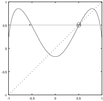
(a) (b)

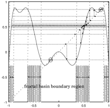
Figure 6: The orbits falling onto unstable fixed point for the spatial map $g^{L}(x)$. All the points on the orbits are the basin boundary points, where the phase of the spatial cycle shows slips. There are 4 such points in the spatial period 2 case (a), and an infinite number in the spatial period 4 case (b).

References

- [1] E.Lifshitz and L.Pitaevskii, Physical Kinetics (1981).
- [2] P.Huerre, in Instabilities and Nonequilibrium Structures (ed. E.Tirapegui and D.Villaroel, Reidel 1987) 141.
- [3] R.J.Deissler, J.Stat.Phys. 54 1459 (1989); 40 371 (1985).
- [4] R.J.Deissler and K.Kaneko, Phys Lett 119A 397 (1987).
- [5] K.Kaneko, Physica D 23 436 (1986).
- [6] K.Fujimoto and K.Kaneko, Physica D 129 203 (1999).
- [7] R.J.Deissler, Phys Lett 100A 451 (1984).
- [8] K.Kaneko, Phys Lett 111A 321 (1985).
- [9] F.H.Willeboordse and K.Kaneko, Physica D 86 428 (1995), and references cited therein.
- [10] J.P.Crutchfield and K.Kaneko, in Directions in Chaos (ed. B.L.Hao, World Scientific 1987) 272.
- [11] R.Carretero-Gonzalez, D.K.Arrowsmith and F.Vivaldi, Physica D 103 381 (1997).
- [12] Here we apply the noise to all elements. However, the noise only to the upstream is essential. In fact, we obtain the same results, even for a system with a noise only at the boundary .
- [13] D.Vergni, M.Falcioni, and A.Vulpiani, Phys.Rev.E. 56 6170 (1997).
- [14] C. Grebogi, E. Ott, and J.A. Yorke, Phys.Rev.Lett. 50 935 (1983); Physica D 24 243 (1987); S. Takesue and K. Kaneko, Prog.Theor.Phys. 71 35 (1984).
- [15] Of course, dependence on the boundary value with a finer scale than the applied noise is blurred. Since the noise has to exist to establish a finite , the self-similar structure is seen only down to , (which is typically very small).
- [16] A.B.Rovinsky and M.Menzinger, Phys.Rev.Lett. 69 1193 (1992); 70 778 (1993); R.Satnoianu, J.Merkin and S.Scott, Phys.Rev.E. 69 (1998) 3246.
- [17] K.Otsuka and K.Ikeda, Phys.Rev.A 39 5209 (1989).
(a) (b)
(b)