Can Strange Nonchaotic Dynamics be induced through Stochastic Driving?

Abstract

Upon addition of noise, chaotic motion in low–dimensional dynamical systems can sometimes be transformed into nonchaotic dynamics: namely, the largest Lyapunov exponent can be made nonpositive. We study this phenomenon in model systems with a view to understanding the circumstances when such behaviour is possible. This technique for inducing “order” through stochastic driving works by modifying the invariant measure on the attractor: by appropriately increasing measure on those portions of the attractor where the dynamics is contracting, the overall dynamics can be made nonchaotic, however not a strange nonchaotic attractor. Alternately, by decreasing measure on contracting regions, the largest Lyapunov exponent can be enhanced. A number of different chaos control and anticontrol techniques are known to function on this paradigm.

I Introduction

The effect of noise on the dynamics of low–dimensional nonlinear systems has been widely studied. One major motivation has been to verify the robustness of observed dynamical phenomena [1, 2], but a large number of studies are directed toward studying whether additive (or multiplicative) noise can induce novel dynamical phenomena.

In this context, noise–induced ordering has been extensively explored in the past few years [3, 4, 5, 6, 7]. At first glance, such results appear counterintuitive since the addition of randomness would normally be expected to enhance the effects of chaos in any system. At the same time, it is well–established that additive noise causes phenomena such as stochastic resonance [8], or otherwise stabilizes chaotic motion [9]. In other situations the effect is to reduce the value of the largest Lyapunov exponent (LE), namely to make the system less chaotic [10], or to create new random attractors [11].

Can strange nonchaotic attractors (SNAs) [12, 13] be formed via stochastic driving of a nonlinear system? While it has been suggested [10] that additive noise can create SNAs, this question touches upon an important open issue. The only examples of SNAs known to date have quasiperiodic driving in the dynamics [13], although there are some experimentally studied systems [14, 15] where the dynamics appears to be on strange nonchaotic attractors, but where there is no explicit quasiperiodic driving. This question therefore has considerable practical relevance.

In this article we examine the mechanism whereby the addition of a chaotic or stochastic signal to a general chaotic system has the effect of reducing the degree of disorder [10]. The particular systems where this occurs all appear to have large contracting regions in the phase space, typified by, say, an exponential tail in the Poincaré map. An additional motivation here is to understand the different mechanisms [4, 7] through which chaotic attractors are “made” nonchaotic. The contrast here is with quasiperiodically driven chaotic dynamical systems which can often transform a strange chaotic attractor into a strange nonchaotic one [12, 13]. On strange nonchaotic attractors (SNAs) the dynamics is aperiodic since the attractor is fractal, but the largest Lyapunov exponent is nonpositive, so there is no sensitivity to initial conditions. The dynamics is intermediate between quasiperiodic and chaotic; there are features of both regularity and chaos.

Our present results suggest that stochastic driving alone cannot create SNAs: noise–induced stabilization differs in important respects from strange nonchaotic dynamics. We find that the noise induced order proceeds as follows. By adding noise, the invariant measure on the (noisy) attractor is modified. If the measure on those regions where the dynamics is locally contracting is enhanced, then this has the effect of lowering the Lyapunov exponent. (Alternately, the Lyapunov exponent can be enhanced by increasing the measure in regions where the local dynamics is expanding). On the other hand, given a quasiperiodically driven system where there are strange nonchaotic attractors, the addition of noise may also destroy such attractors [16].

Our main results are presented in Section II, where we discuss model systems with stochastic forcing. We analyse the dynamics in terms of local Lyapunov exponents [16, 17] and show the methodology of this mechanism for inducing ordering. A number of previously studied control methods [18, 19, 20] appear to fall in this class of techniques, as does a related anticontrol method [21]. A summary follows in Section III.

II Results

Consider a stochastically driven nonlinear dynamical system specified by, say, the iterative mapping

$$x_{n+1}=f(x_{n})+\sigma\xi_{n},$$ (1)

where $\xi_{n}$ is additive stochastic or random noise of strength $\sigma$. We consider the case when the system has positive Lyapunov exponent with no driving, i.e. for $\sigma=0$. For nonzero $\sigma$ it can happen [10] that the Lyapunov exponent corresponding to the $x$ degree of freedom

$$\lambda=\lim_{N\to\infty}{1\over N}\sum_{i=1}^{N}\ln|f^{\prime}(x_{i})|$$ (2)

can become negative.

A number of related situations show a very similar property, namely that the Lyapunov exponent decreases on addition of an extra stochastic or chaotic term in the dynamics. For example, driving via another chaotic system,

$$x_{n+1} = f(x_{n})+\sigma\xi_{n}$$ (3)

$$\xi_{n+1} = g(\xi_{n}),$$ (4)

where the maps $f$ and $g$ can be different from each other, or in an extreme case, where $\xi_{n}$ is a constant, namely the case of constant feedback studied in some detail by Parthasarathy and Sinha [20]. This type of feedback causes the system, Eq. (1) to display a form of “control”. It may happen that a periodic orbit is stabilized via feedback [18, 19, 20]. Alternately, the motion continues to be aperiodic, but since the Lyapunov exponent is negative, two systems with different initial conditions which are driven by the exactly same noise will actually show synchronization.

However, in a trivial sense, the above dynamical system cannot possess a nonchaotic attractor because the largest Lyapunov exponent, namely that corresponding to the $\xi$ degree of freedom is positive. If one considers two separate initial conditions, namely driving two systems with independent realizations of the noise or chaotic driving, then there is no synchronization, as can be expected. In this feature, such dynamics differs from the motion on strange nonchaotic attractors where there can be robust synchronization [22]. One cannot have true SNA dynamics in the presence of stochastic driving alone.

Some understanding of the above results can be obtained by considering typical examples [3, 10]. For specific maps considered the exponential logistic map,

$$x_{n+1}\equiv F(x_{n})=x_{n}\exp[\alpha(1-x_{n})].$$ (5)

and the quadratic logistic map,

$$x_{n+1}\equiv F(x_{n})=\alpha^{\prime}x_{n}(1-x_{n}),$$ (6)

These show the typical bifurcation diagram as a function of $\alpha$  or  $\alpha^{\prime}$, with chaotic dynamics over a range in parameter space. In the latter case, Eq. (6), e. g.  at $\alpha^{\prime}=4$, it is observed [3, 6] that on adding the restricted noise [23] the LE does not decrease: a pair of such chaotic systems synchronize with identical driving noise [3]. The logistic map also synchronizes with restricted noise, and in this case, the Lyapunov exponent remains positive [6].

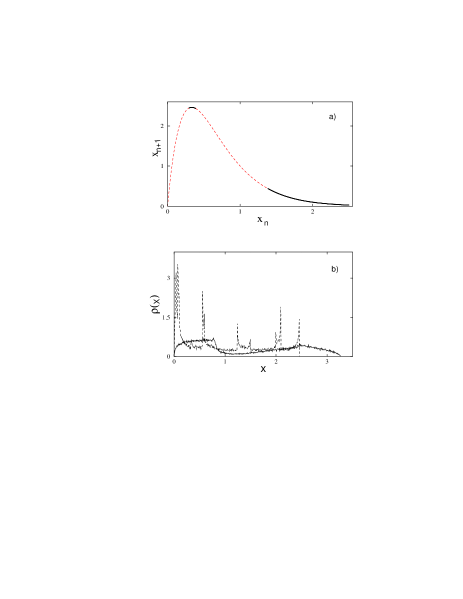
FIG. 1.: (a) The exponential logistic map with $\alpha=3$. Here, the dashed lines are the expanding regions of the map, $|f^{\prime}(x)|>1$, and the solid lines are the contracting regions. (b) The invariant density $\rho(x)$ at $\alpha=3$ with noise strength $\sigma=0$ (dashed line) and $\sigma=0.1$ (solid line). The noise is $\delta$-correlated white noise.

Both maps have contracting and expanding sub–regions but behave in different ways. This difference can be analysed by considering Eq. (5), for instance, at $\alpha=3$; the dynamics is chaotic for almost every initial condition on $[0,\infty]$. Beyond $x\approx 1.4$ and in the region around the map maximum [Fig. 1(a)], the map is contracting, so that only a small region of the phase space is effectively responsible for the chaotic dynamics. Most of the natural invariant measure is, however, concentrated away from these contracting regions; see Fig. 1(b). However for Eq. (6), the phase space is restricted only to [0,1] and the contracting region is relatively much narrower.

The mapping Eq. (5) has positive Lyapunov exponent for $\alpha=3$. By adding a noise term as in Eq. (1), the natural measure can be modified so as to increase the sampling of the contracting regions of phase space [Fig. 1(b)]: this reduces the Lyapunov exponent of the driven system. Consider the partial sums,

$$\lambda_{+}=\lim_{N_{+}\to\infty}{1\over N_{+}}\sum_{i}\ln|f^{\prime}(x_{i})|,~{}~{}~{}~{}~{}~{}|f^{\prime}(x_{i})|>1,$$ (7)

and

$$\lambda_{-}=-\lim_{N_{-}\to\infty}{1\over N_{-}}\sum_{i}\ln|f^{\prime}(x_{i})|,~{}~{}~{}~{}~{}~{}|f^{\prime}(x_{i})|<1,$$ (8)

namely the separate contributions to the Lyapunov exponent. These are obtained by partitioning a long trajectory ($N\to\infty$) into $N_{+}$ points on expanding regions and $N_{-}$ points on contracting regions. Clearly, $N=N_{+}+N_{-}$ and $\lambda=\frac{N_{+}}{N}\lambda_{+}-\frac{N_{-}}{N}\lambda_{-}$. As the intensity of the noise term increases, the dynamics is pushed out onto those parts of phase space where the average slope of the map is less than 1. Thus the latter partial sum, $\lambda_{-}$, increases in magnitude at the expense of $\lambda_{+}$ and eventually becomes larger than $\lambda_{+}$, leading to a Lyapunov exponent which is zero or negative. The variation of these quantities with noise strength $\sigma$ is shown in Fig. 2, and it is clear that the system can be made “nonchaotic” both in the case of additive noise, as well as for driving via an added chaotic signal.

FIG. 2.: The Lyapunov exponent (solid line) and its partial sums, $\lambda_{+}$ (dashed) and $\lambda_{-}$ (dots) [see Eqs. (7) and (8) respectively] as a function of the noise strength $\sigma$.

Similar ideas apply to noise–driven flows where analogous results can be obtained. Again, we find that systems where the Lyapunov exponents can be reduced by adding noise are characterized by having a large contracting region in the phase space; this can be detected by examination of the return map, for instance. An important class of such continuous system that we have studied are equations corresponding to the kinetics of coupled chemical reactions, as for example the cubic non-isothermal autocatalator (see Chapter 4 in Ref. [24] and references therein for more details).

$$\frac{dx}{dt} = \mu\exp(z)-xy^{2}-\kappa x$$ (9)

$$\frac{dy}{dt} = xy^{2}+\kappa x-y$$ (10)

$$\frac{dz}{dt} = \delta y-\gamma z$$ (11)

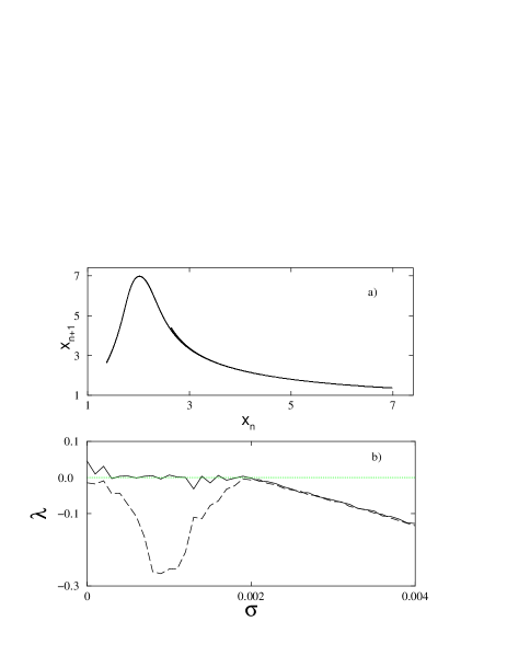
FIG. 3.: (a) Return map for the chemical reaction system, Eq. (11) with parameters $\mu=0.707,\kappa=0.00055,~{}\delta=0.1$,  and  $\gamma=0.5$ in the absence of noise; and (b) the variation of the largest two Lyapunov exponents for Eq. (11) as a function of the strength of added noise, $\sigma$.

Shown in Fig. 3(a) is the return map for the system in the regime where the dynamics is chaotic, which shows an exponential tail similar to the simple iterative mapping, Eq. (5). Upon addition of noise the Lyapunov exponents decreases as shown in Fig. 3(b). Other examples with very similar behaviour in higher dimensions are, for example, equations that model the Belousov-Zhabotinsky reaction [24, 25, 26]. Since these reactions can be studied experimentally, it is possible that the effect of noise in reducing chaos in such systems can be verified in practice [25].

A number of different systems which share the above features [10, 25, 27] can be controlled in this manner, namely by adding noise or chaotic driving. Note, however, that the system is not truly “nonchaotic”. Unlike the dynamics on periodic or quasiperiodic attractors or SNAs where all the Lyapunov exponents are nonpositive, here the dynamics is not confined to a single global attractor, but to some region of the phase space for each realization of noise. Therefore the fluctuations of all dynamical quantities, and in particular the Lyapunov exponents, actually increase because of the additive noise.

III Summary

Nonuniform attractors in nonlinear dynamical systems typically have interwoven contracting and expanding subregions. By increasing the measure on regions where the dynamics is locally contracting relative to those which are locally unstable, one can render the motion “nonchaotic”. This can be effected through the action of additive noise: the invariant measure on some chaotic attractors can be so modified [5, 10] that the dynamics is taken to those regions of the attractor which are contracting on average, and this results in a nonpositive Lyapunov exponent. Indeed, noisy experimental data can yield a negative value for the Lyapunov exponent even though the actual dynamics of the system may be chaotic.

Adding stochastic noise, does not, however, create strange nonchaotic attractors [12]. For each realization of the noise, the limiting set is different, and thus there are no attractors per se. One important property of SNAs is the synchronization of two trajectories driven by the same external quasiperiodic force [22]. Motion on the nonchaotic sets obtained by adding noise do not have this property unless they are driven by identical noise. Whether it is reasonable to expect that this can be realized in practice is a moot question.

In the present work, we have considered only additive stochastic driving. It is possible that some other forms of stochastic driving (perhaps via parametric modulation) can create true SNAs; this question remains to be explored.

ACKNOWLEDGMENT

This research has been supported by a grant from the Department of Science and Technology, India.

REFERENCES

- [1] J. Crutchfield, D. Farmer, and B. Huberman, Phys. Rep., 92, 42 (1982).
- [2] See e. g. T. Kapitaniak, Chaos in systems with Noise, (World Scientific, Singapore, 1990).
- [3] A. Maritan and J. R. Banavar, Phys. Rev. Lett., 72, 1451 (1994). See also A. Pikovsky, Phys. Rev. Lett., 73, 2931 (1994) and A. Maritan and J. Banavar, Phys. Rev. Lett., 73, 2932 (1994).
- [4] S. Fahy and D. R. Hamann, Phys. Rev. Lett., 69, 761 (1992).
- [5] K. Matsumoto and I. Tsuda, J. Stat. Phys., 31, 87 (1983).
- [6] L. Longa, S. P. Dias, and E. M. F. Curado, Phys. Rev. E, 56, 259 (1997).
- [7] A. S. Pikovsky, Phys. Lett. A, 165, 33 (1992).
- [8] See e. g. L. Schimansky-Geier, J. A. Freund, A. B. Neiman, and B. Shulgin, Int. J. Bifurcation and Chaos, 8, 869 (1998); J. Stat. Phys., 70, 1 (1993).
- [9] R. Wackerbauer, Phys. Rev. E, 52, 4745 (1995).
- [10] S. Rajasekar, Phys. Rev. E, 51, 775 (1995).
- [11] P. Ashwin, Physica D, 125, 302 (1999).
- [12] C. Grebogi, E. Ott, S. Pelikan, and J. A. Yorke, Physica D, 13, 261 (1984).
- [13] A. Prasad and R. Ramaswamy, to be published.
- [14] A. J. Mandell and K. A. Selz, J. Stat. Phys., 70, 255 (1993).
- [15] W. X. Ding, H. Deutsch, A. Dinklage, and C. Wilke, Phys. Rev. E, 55, 3769 (1997).
- [16] A. Prasad, V. Mehra, and R. Ramaswamy, Phys. Rev. E, 57, 1576 (1998).
- [17] H. D. I. Abarbanel, R. Brown, and M. B. Kennel, J. Nonlinear Sci. 2, 343 (1991).
- [18] E. R. Hunt, Phys. Rev. Lett., 67, 1953 (1991).
- [19] J. Güémez and M. Matías, Phys. Lett. A, 181, 29 (1993).
- [20] S. Parthasarathy and S. Sinha, Phys. Rev. E, 51, 6239 (1995).
- [21] R. E. Amritkar and N. Gupte, Phys. Rev. E, 54, 4580 (1996).
- [22] C. Zhou and T. Chen, Europhys. Lett. 38, 261 (1997); R. Ramaswamy, Phys. Rev. E, 56, 7294 (1997).
- [23] The random numbers, , are chosen such that the final value, remains in .
- [24] S. K. Scott, Chemical Chaos, (Clarendon Press, Oxford,1993) and references therein.
- [25] K. G. Coffman, W. D. McCormick, Z. Noszticzius, R. H. Simoyi, and Harry L. Swinney, J. Chem. Phys. 86, 119 (1987).
- [26] P. Richetti, J. C. Roux, F. Argoul, and A. Arneodo, J. Chem. Phys. 86, 3339 (1987).
- [27] P. C. Hemmer, J. Phys. A 17, L247 (1984).