Relaxation to the Invariant Density for the Kicked Rotor

Abstract

The relaxation rates to the invariant density in the chaotic phase space component of the kicked rotor (standard map) are calculated analytically for a large stochasticity parameter, $K$. These rates are the logarithms of the poles of the matrix elements of the resolvent, $\hat{R}(z)=(z-\hat{U})^{-1}$, of the classical evolution operator $\hat{U}$. The resolvent poles are located inside the unit circle. For hyperbolic systems this is a rigorous result, but little is known about mixed systems such as the kicked rotor. In this work, the leading relaxation rates of the kicked rotor are calculated in presence of noise, to the leading order in $1/\sqrt{K}$. Then the limit of vanishing noise is taken and the relaxation rates are found to be finite, corresponding to poles lying inside the unit circle. It is found that the slow relaxation rates, in essence, correspond to diffusion modes in the momentum direction. Faster relaxation modes intermix the motion in the momentum and the angle space. The slowest relaxation rate of distributions in the angle space is calculated analytically by studying the dynamics of inhomogeneities projected down to this space. The analytical results are verified by numerical simulations.

PACS number(s): 05.45.-a, 05.45.Ac

I Introduction

For chaotic systems specific trajectories are extremely complicated and look random  [1]. Therefore it is natural to explore the statistical properties of such systems. For this purpose the evolution of probability densities of trajectories in phase space is studied  [2, 3, 4]. For chaotic systems the probability densities, approach an equilibrium density that depends only on the system and not on the initial density. For hyperbolic systems (A systems), like the baker map, the relaxation is exponential. For such systems the existence of the relaxation rates was rigorously established and the relaxation rates are the Ruelle resonances  [5, 6, 7]. To study these rates it is instructive to introduce the evolution operator of densities that is sometimes called the Frobenius-Perron (FP) operator. Relaxation to the equilibrium density is studied traditionally in statistical mechanics. In particular for particles performing a random walk in a finite box, relaxation to the equilibrium uniform density takes place and is governed by the rate related to the lowest nontrivial mode of diffusion equation. It is known that for the classical kicked rotor, described by the standard map, diffusive spread in phase space takes place for a sufficiently large stochasticity parameter  [8, 9]. Therefore it is natural to study the Frobenius-Perron (FP) operator for the kicked rotor and to compare it to the diffusion operator, a comparison that enables to study some aspects of chaotic dynamics in the framework of statistical mechanics  [10]. The kicked rotor model is a paradigm for the chaotic behavior of systems where one variable is unbounded in the phase space. For such classical systems diffusive spreading takes place. For their quantum counterparts it is suppressed by interference effects, leading to a mechanism that is similar to Anderson localization in disordered solids  [11, 12, 13].

The kicked rotor is defined by the Hamiltonian (in appropriate units)

$${\cal{H}}=\frac{1}{2}J^{2}+Kcos\theta\sum_{n}\delta(t-n),$$ (1)

where $J$ is the angular momentum, $\theta$ is the conjugate angle $(0\leq\theta<2\pi)$ and $K$ is the stochasticity parameter. Since the angular momentum between the kicks is conserved, the equation of motion generated by (1) reduces to a map, known as the standard map

$$\bar{\theta}=\theta+\bar{J}$$ (2)

$$\bar{J}=J-Ksin\theta,$$ (3)

where $\theta$ and $J$ are the angle and the angular momentum before the kick, while $\bar{\theta}$ and $\bar{J}$ are these quantities just before the next kick. For $K>K_{c}\approx 0.9716$ diffusion in phase space is found, and for large $K$ the diffusion coefficient is given by an expansion in $\frac{1}{\sqrt{K}}$ as:  [14]

$$D(K)=\frac{K^{2}}{4}\left(1-2J_{2}(K)+...\right).$$ (4)

To be precise it was shown that after a large number of kicks, n, the variance of the momentum behaves as:

$$\langle(J-\langle J\rangle)^{2}\rangle\sim 2Dn,$$ (5)

where $\langle\cdots\rangle$ denotes an averaging over the angle initial distribution, and $D$ is given by (4).

It is assumed that the system evolves in presence of finite noise and the limit of the vanishing noise is taken in the end of the calculation. The noise is required here in order to get well defined results. It leads to escape from the accelerator modes and other stable islands. Accelerator modes, where the angular momentum $J$ grows linearly with time, are found for values of $K$ and the initial values ($\theta_{0}$,$J_{0}$) of the angle and the angular momentum, that satisfy $Ksin\theta_{0}=2\pi l_{0}$ and $J=2\pi l$ where $l$ and $l_{0}$ are integers. In such a situation at each step, $J$ grows by $2\pi l_{0}$, as is obvious from (2) and (3), namely its growth is linear in time. For some values of $K$ the point ($\theta_{0}$,$J_{0}$) is stable and also for initial conditions in its vicinity the momentum grows linearly. This differs from diffusion, that takes place in the chaotic component of phase space. For trajectories in the chaotic component of phase space noise avoids long time sticking in the vicinity of islands of stability  [15]. In numerical calculations without noise diffusion is found for $K>K_{c}$ for trajectories in the extended chaotic component for large values of $K$, but also some exceptions were reported  [15]. The diffusion coefficient (4) was calculated in presence of finite noise (in the long time limit) and the limit of the vanishing noise can be taken in the end of the calculation [14]. It describes the typical spreading of trajectories in the chaotic component. Since the kicked rotor is a mixed system, as is the case for most physical examples, the rigorous mathematical theory for relaxation  [5, 3, 2] does not apply and one has to resort to heuristic methods.

In the present paper [16] the Frobenius-Perron operator will be calculated for the kicked rotor on the torus:

$$\ \ \ (0\leq J<2\pi s)\\$$ (6)

$\displaystyle(0\leq\theta<2\pi),$

where $s$ is integer. This is reasonable since the map (2-3) is $2\pi$ periodic both in $J$ and in $\theta$. The operator is defined in the space spanned by the Fourier basis

$$\phi_{km}=(J\theta|km)=\frac{1}{\sqrt{2\pi}}\frac{1}{\sqrt{2\pi s}}\exp(im\theta)\exp\left(i\frac{kJ}{s}\right).$$ (7)

Note that the functions $\phi_{k0}$ form the basis of eigenstates of the diffusion operator in the angular momentum $J$. The FP operator for an area preserving invertible map,

$\displaystyle\bar{\bf x}=M({\bf x})$

is

$$\hat{U}\rho(\theta,J)=\rho(M^{-1}(\theta,J)).$$ (8)

It was studied rigorously for the hyperbolic systems and many of its properties are known  [2, 3, 5, 17, 18]. It is a unitary operator in ${\cal L}^{2}$, the Hilbert space of square integrable functions. Therefore its resolvent

$$\hat{R}(z)=\frac{1}{z-\hat{U}}=\frac{1}{z}\sum_{n=0}^{\infty}\hat{U}^{n}z^{-n}$$ (9)

is singular on the unit circle in the complex $z$ plane. The matrix elements of $\hat{R}$ are discontinuous there and one finds a jump between two Riemann sheets. This results from the fact that the spectrum is continuous and infinitely degenerate  [2]. The sum (9) is convergent for $|z|>1$, therefore it identifies the physical sheet, as the one connected with the region $|z|>1$. (This is analogous to the sign of the small imaginary increment in the energy that is used in the definition of the Green function). The Ruelle resonances are the poles of the matrix elements of the resolvent, on the Riemann sheet, extrapolated from $|z|>1$  [17]. These describe the decay of smooth probability distribution functions to the invariant density in a coarse grained form  [3, 5]. Even a smooth initial distribution will develop complicated patterns as a result of the evolution of a chaotic map. The Ruelle resonances describe the decay of its coarse grained form to the invariant density. In spite of the solid mathematical theory there are very few examples where the Ruelle resonances were calculated for specific systems. They were calculated analytically for the baker map where the basis of Legendre polynomials was used  [17] and various of its variants  [3]. The Ruelle resonances were calculated also for the “cat” map and some of its variants  [18]. Blum and Agam applied a variational method for the calculation of the leading Ruelle resonances of the “perturbed cat” map, and the results were verified numerically[19]. In addition they calculated the leading resonances of the standard map with $s=1$ for various values of the stochasticity parameter $K$. The leading Ruelle resonances for the kicked top were calculated by Weber, Haake and Šeba  [20] with the help of a combination of a cycle expansion and numerical calculations. The resonances mentioned above are not related to the spectrum of the Liouville operator that is confined to the unit circle because of its unitarity.

In the present work, the FP operator is calculated for the kicked rotor. Here the classical evolution operator, for one time step, can be written in the form

$$\hat{U}_{KR}=\delta(\bar{\theta}-\theta-\bar{J})\delta(\bar{J}-J+Ksin\theta),$$ (10)

and its operation on a phase space density $\rho$ is

$$\hat{U}\rho(\theta,J)=\rho(\theta-J,J+Ksin(\theta-J)).$$ (11)

To make the calculation well defined noise is added to the system. It is shown that the noise acts effectively as coarse graining and the resulting FP operator is not unitary (see also  [21]). For large stochasticity parameter $K$, we show that the slowest relaxation modes in the limit of infinitesimal noise are the modes of the diffusion operator in the angular momentum space. Also calculated is the slowest rate of relaxation in the angle space. The approximate analytical results are tested numerically.

It is understood that the noise is kept finite when the limits of large $K$ and $s$ are taken and then the limit of zero noise is taken. The natural question is whether it is possible that this description, which was established only for hyperbolic systems, holds also for mixed systems. Clearly, for mixed systems it can be only approximate. It holds for large values of the stochasticity parameter $K$ since then most of the phase space is covered by the chaotic component. For smaller values of $K$ the weight of the regular regions increases. In such a situation, in the limit of increasing resolution the resonances related to the regular component are expected to move to the unit circle in the complex $z$ plane, corresponding to the quasi-periodic motion, while the resonances associated with the chaotic component stay inside the unit circle. This was found by Weber, Haake and Šeba  [20] for the kicked top that is a mixed system.

How is the FP operator related to the quantum mechanical evolution operator? It was shown numerically for the baker map that if both operators are calculated with finite resolution they exhibit the same Ruelle resonances  [21]. In this calculation it was assumed that the phase space coarse graining tends to zero in the semi-classical limit $\hbar\rightarrow 0$. It was shown by Zirnbauer  [22] that some noise is required for a meaningful definition of the field theories introduced to study level statistics for chaotic systems  [23]. This noise affects only quantum properties, therefore the resulting ensemble has the same classical FP operator. The localization length of the kicked rotor calculated from this field theory  [24] is related to the classical FP operator. This operator is analyzed in the present work, clarifying some issues of that work. The results hold only for typical quantum systems, since the noise introduced in the present work as well as the noise required for the stabilization of the field theory  [22] washes out the sensitive quantum details such as the number theoretical properties of the effective Planck constant  [25].

The Frobenius-Perron operator in the basis (7) in the presence of noise is defined and calculated in Sec. 2, its Ruelle resonances are obtained within some approximations in Sec. 3 and their regime of validity is tested numerically in Sec. 4. The results are summarized and discussed in Sec. 5.

II The evolution operator of phase space distributions

In this section the evolution operator of phase space densities of the kicked rotor in presence of some type of noise is derived. The noise is added to the free motion part (2). In the absence of noise the phase space evolution of a distribution $f$ is given by Liouville equation

$$\frac{df}{dt}=\frac{\partial f}{\partial t}+\dot{\theta}\frac{\partial f}{\partial\theta}+\dot{J}\frac{\partial f}{\partial J}=0.$$ (12)

If noise that conserves J, and leads to diffusion in $\theta$, is added to the free motion, equation (12) should be replaced by

$$\frac{\partial f}{\partial t}+J\frac{\partial f}{\partial\theta}-\frac{\sigma^{2}}{2}\frac{\partial^{2}f}{\partial\theta^{2}}=0,$$ (13)

where $J=\dot{\theta}$ was used. It can be written as:

$$\frac{\partial f}{\partial t}=\hat{A}f,$$ (14)

where the operator $\hat{A}$ is:

$$\hat{A}=-J\frac{\partial}{\partial\theta}+\frac{\sigma^{2}}{2}\frac{\partial^{2}}{\partial\theta^{2}}.$$ (15)

The complete set of its eigenfunctions is given by $\varphi_{m}=\frac{1}{\sqrt{2\pi}}\exp(im\theta)$, where $m$ is integer. The operator we need is  $\hat{U}_{noise}=e^{\hat{A}}$, and explicitly

$$(J^{\prime}\theta^{\prime}|\hat{U}_{noise}|J\theta)=\sum_{m}\varphi_{m}(\theta^{\prime})\varphi_{m}^{*}(\theta)\exp(\alpha_{m})\delta(J-J^{\prime}),$$ (16)

where the $\alpha_{m}$ are the eigenvalues of the operator $\hat{A}$, namely $\hat{A}|\varphi_{m})=\alpha_{m}|\varphi_{m})$. Obviously

$$\alpha_{m}=-imJ-\frac{\sigma^{2}}{2}m^{2}$$ (17)

leading to

$$(J^{\prime}\theta^{\prime}|\hat{U}_{noise}|J\theta)=\sum_{m}\frac{1}{2\pi}\exp\left(im(\theta^{\prime}-\theta-J)-\frac{\sigma^{2}}{2}m^{2}\right)\delta(J-J^{\prime}).$$ (18)

The $\delta$-function in momentum reflects the fact that the noise does not affect the momentum. The matrix elements $(k_{2}m_{2}|\hat{U}|k_{1}m_{1})$ of evolution operator $\hat{U}$ in the Fourier basis (7) will be calculated in two steps, first the contribution of the kick, and then the one of the free motion with noise will be calculated. According to (3) and (11), the kick transforms the state $(\theta,J|k_{1}m_{1})=\frac{1}{\sqrt{2\pi}}\frac{1}{\sqrt{2\pi s}}\exp(im_{1}\theta)\exp\left(i\frac{k_{1}J}{s}\right)$ to the state

$$\frac{1}{\sqrt{2\pi}}\frac{1}{\sqrt{2\pi s}}\exp(im_{1}\theta)\exp\left(i\frac{k_{1}}{s}(J+Ksin\theta)\right)\equiv(\theta,J|\hat{U}_{K}|k_{1}m_{1}).$$ (19)

Adding the effect of noise yields the matrix element in the mixed representation

$$(J\theta|\hat{U}|k_{1}m_{1})=\int_{0}^{2\pi}d\theta^{\prime}\int_{0}^{2\pi s}dJ^{\prime}(J\theta|\hat{U}_{noise}|J^{\prime}\theta^{\prime})(J^{\prime}\theta^{\prime}|\hat{U}_{K}|k_{1}m_{1}).$$ (20)

Its transformation to the basis (7) is calculated in App. A and the result is

$$(k_{2}m_{2}|\hat{U}|k_{1}m_{1})=J_{m_{2}-m_{1}}\left(\frac{k_{1}K}{s}\right)\exp\left(-\frac{\sigma^{2}}{2}m_{2}^{2}\right)\delta_{k_{2}-k_{1},m_{2}s}.$$ (21)

For $\sigma=0$, using (21) one can verify by a straightforward summation that $\hat{U}^{\dagger}\hat{U}=I$, therefore the operator is unitary as required.

Some of the eigenfunctions of $\hat{U}$ in the limit $\sigma=0$ are easily found. It is convenient to use the representation (10) of $\hat{U}$. We guess an eigenfunction of the form

$$F(\theta,J)=\delta(\theta-\theta_{0})\sum_{l}\exp(iqJ/s)\delta(J-2\pi l)$$ (22)

with q integer satisfying $1\leq q\leq s$. These are functions localized on accelerator modes representing linear growth of the angular momentum with time. To check that these are indeed eigenfunctions we note that

$$\hat{U}_{KR}F(\theta,J)=\delta(\theta-J-\theta_{0})\sum_{l}\delta(J+Ksin\theta_{0}-2\pi l)\exp\left(i\frac{q}{s}(J+Ksin\theta_{0})\right)$$ (23)

taking $\theta_{0}$ so that

$\displaystyle Ksin\theta_{0}=2\pi l_{0},$

where $l_{0}$ is integer yields

$$\hat{U}_{KR}F(\theta,J)=e^{i2\pi ql_{0}/s}F(\theta,J),$$ (24)

since the RHS of (23) does not vanish only for $J=2\pi l$. The eigenvalues $e^{i2\pi ql_{0}/s}$ lie on the unit circle and become dense as $s\rightarrow\infty$. There are more eigenfunctions of this form located on other periodic orbits  [26].

III Identification of the Ruelle resonances

The purpose of this section is to calculate the Ruelle resonances for the kicked rotor with the help of Frobineus-Perron operator (21). The calculation will be done for finite noise $\sigma$ and then the limit $\sigma\rightarrow 0$ will be taken. The Ruelle resonances are the poles of matrix elements of the resolvent operator $\hat{R}$ of (9),

$$R_{12}=(k_{1}m_{1}|\hat{R}(z)|k_{2}m_{2})=\left(k_{1}m_{1}\left|\frac{1}{z-\hat{U}}\right|k_{2}m_{2}\right),$$ (25)

when analytically continued from outside of the unit circle in the complex plane. It is useful to introduce the operator

$$\hat{R}^{\prime}(z)=\frac{1}{1-z\hat{U}},$$ (26)

that is related to the resolvent by

$$\frac{1}{z}\hat{R}^{\prime}\left(\frac{1}{z}\right)=\hat{R}(z)$$ (27)

and

$$\frac{1}{z}\hat{R}\left(\frac{1}{z}\right)=\hat{R}^{\prime}(z).$$ (28)

The matrix elements of $\hat{R}$ and $\hat{R}^{\prime}$ satisfy similar relations. Continuing the matrix elements of $\hat{R}(z)$ from outside to inside of unit circle is equivalent to continuing the matrix elements of $\hat{R}^{\prime}(z)$ from inside to outside of unit circle. The last continuation is easier to study since the expansion

$$\hat{R}^{\prime}(z)=\frac{1}{1-z\hat{U}}=\sum_{n=0}^{\infty}z^{n}\hat{U}^{n}$$ (29)

is convergent inside the unit circle, because

$$||z\hat{U}||\leq 1.$$ (30)

The resulting matrix elements are

$$R^{{}^{\prime}}_{12}=(k_{1}m_{1}|\hat{R}^{\prime}(z)|k_{2}m_{2})=\sum_{n=0}^{\infty}a_{n}z^{n},$$ (31)

where

$$a_{n}=(k_{1}m_{1}|\hat{U}^{n}|k_{2}m_{2}).$$ (32)

Through (27) and (28) this expansion is related to matrix elements outside of the unit circle. If $z_{c}$ is a singularity of $R_{12}$ then $1/z_{c}$ is a singular point of $R^{{}^{\prime}}_{12}$. Consequently the first singularity of the analytic continuation of $R^{{}^{\prime}}_{12}(z)$ from inside to outside the unit circle gives the first singularity one encounters when analytically continuing $R_{12}(z)$ from outside to inside the unit circle, i.e. it is just the leading nontrivial resonance. This is the most interesting resonance determining the relaxation to the invariant density. The first singularity in the extrapolation of the matrix elements of $\hat{R}^{\prime}$ from inside to outside the unit circle is determined from the fact that it is the radius of convergence of this series. Moreover according to the Cauchy-Hadamard theorem (see  [27]) the inverse of the radius of convergence is given by

$$r^{-1}=\lim_{n\rightarrow\infty}\sup\sqrt[n]{|a_{n}|}.$$ (33)

If $a_{n}\sim c/r^{n}$ we may say that the radius of convergence is the asymptotic value of $a_{n-1}/a_{n}$. This is the basis for the ratio method for determining the radius of convergence. The resonance that is closest to the unit circle can be identified from the radius of convergence.

We turn now to calculate the coefficients $a_{n}$. First the matrix elements $(k0|\hat{R}^{\prime}(z)|k0)$ will be calculated. For these the expansion coefficients are:

$$a_{n}=(k0|\hat{U}^{n}|k0).$$ (34)

Introducing the resolution of the identity,

$$a_{n}=\sum_{k_{1},m_{1}}\sum_{k_{2},m_{2}}...\sum_{k_{n-1},m_{n-1}}(k0|\hat{U}|k_{1}m_{1})(k_{1}m_{1}|\hat{U}|k_{2}m_{2})...(k_{n-1}m_{n-1}|\hat{U}|k0),$$ (35)

and substitution of (21) leads to:

$$a_{n}=\sum_{k_{1},m_{1}}\sum_{k_{2},m_{2}}...\sum_{k_{n-1},m_{n-1}}J_{0-m_{1}}\left(\frac{k_{1}K}{s}\right)\delta_{k-k_{1},0}J_{m_{1}-m_{2}}\left(\frac{k_{2}K}{s}\right)\exp\left(-\frac{\sigma^{2}}{2}m_{1}^{2}\right)\delta_{k_{1}-k_{2},m_{1}s}$$ (36)

$\displaystyle J_{m_{2}-m_{3}}\left(\frac{k_{3}K}{s}\right)\exp\left(-\frac{\sigma^{2}}{2}m_{2}^{2}\right)\delta_{k_{2}-k_{3},m_{2}s}...J_{m_{n-1}-0}\left(\frac{kK}{s}\right)\exp\left(-\frac{\sigma^{2}}{2}m_{n-1}^{2}\right)\delta_{k_{n-1}-k,m_{n-1}s}.$

Summation over the $k_{i}$ yields,

$$a_{n}=\sum_{m_{1}}\sum_{m_{2}}...\sum_{m_{n-1}}J_{0-m_{1}}\left(\frac{kK}{s}\right)$$ (37)

$\displaystyle J_{m_{1}-m_{2}}\left(\frac{kK}{s}-m_{1}K\right)\exp\left(-\frac{\sigma^{2}}{2}m_{1}^{2}\right)J_{m_{2}-m_{3}}\left(\frac{kK}{s}-(m_{1}+m_{2})K\right)\exp\left(-\frac{\sigma^{2}}{2}m_{2}^{2}\right)$

$\displaystyle...J_{m_{n-2}-m_{n-1}}\left(\frac{kK}{s}-(m_{1}+m_{2}+...+m_{n-2})K\right)\exp\left(-\frac{\sigma^{2}}{2}m_{n-2}^{2}\right)$

$\displaystyle J_{m_{n-1}-0}\left(\frac{kK}{s}\right)\exp\left(-\frac{\sigma^{2}}{2}m_{n-1}^{2}\right)\delta_{m_{1}+m_{2}+...+m_{n-2}+m_{n-1},0}.$

Thus in order to obtain the expansion coefficient $a_{n}$ we should perform summation in (37) over all integers subject to the constraint

$$m_{1}+m_{2}+...+m_{n-1}=0.$$ (38)

We are interested in the limit of large $s$ and $K$. The limits are taken in the order

$$(1)\ s\rightarrow\infty,\ (2)\ K\rightarrow\infty,\ (3)\ \sigma\rightarrow 0.$$ (39)

Finite $\sigma$ is required to assure the absolute convergence of the series. Therefore (37) is summed for finite $\sigma$ and the limit $\sigma\rightarrow 0$ should be taken in the end of the calculation. Having this limit in mind the leading term in $K/s$ and $1/\sqrt{K}$ will be identified. It will be assumed that the mode that is calculated is sufficiently low so that

$$0<kK/s<<1.$$ (40)

Each term in (37) is defined by the string

$\displaystyle(m_{1},m_{2},...,m_{i},...,m_{n-1}).$

The leading contribution

$$a_{n}^{(0)}=J_{0}^{n}\left(\frac{kK}{s}\right)\approx\left(1-\frac{k^{2}K^{2}}{4s^{2}}\right)^{n}$$ (41)

results from the string where all $m_{j}$ vanish. A nonvanishing $m_{j}$ results in a Bessel function with a large argument, since $K/s<<1$ and $K>>1$, and therefore it leads to a factor $1/\sqrt{K}$ in the contribution to $a_{n}$. Let $m_{i}$ be the first nonvanishing $m_{j}$ and $m_{f}$ the last nonvanishing one. The first factor in (37) that is not $J_{0}(\frac{kK}{s})$ is $J_{-m_{i}}\left(\frac{kK}{s}\right)$ and the last factor that differs from $J_{0}(\frac{kK}{s})$ is

$$J_{m_{f}}\left(\frac{kK}{s}-(m_{1}+m_{2}+...+m_{f})K\right)=J_{m_{f}}\left(\frac{kK}{s}\right).$$ (42)

Since $J_{n}(x)\approx\frac{x^{n}}{2^{n}n!}$ for small $x$ and $J_{-n}(x)=(-1)^{n}J_{n}(x)$ the contribution of the terms between $i$ and $f$ is of the order

$$C\ \left(\frac{kK}{s}\right)^{|m_{i}|+|m_{f}|}\ ,$$ (43)

where $C$ is the contribution of the factors with $m_{j}$ that are not the first and last ones. The first factor after $m_{i}$ is

$\displaystyle J_{m_{i}-m_{i+1}}\left(\frac{kK}{s}-(m_{1}+...+m_{i})K\right)=J_{m_{i}-m_{i+1}}\left(\frac{kK}{s}-m_{i}K\right)$

and the last factor before $m_{f}$ is

$\displaystyle J_{m_{f-1}-m_{f}}\left(\frac{kK}{s}-(m_{1}+...+m_{f-1})K\right)=J_{m_{f-1}-m_{f}}\left(\frac{kK}{s}-(m_{i}+...+m_{f-1})K\right).$

The terms in between are of the form $J_{m_{j-1}-m_{j}}\left(\frac{kK}{s}-M_{j}K\right)$, where $M_{j}=m_{i}+m_{i+1}+...m_{j}\neq 0$ that are of the order $1/\sqrt{K}$. Therefore the largest contribution from a string $m_{i},m_{i+1},...,m_{f}$ is from the shortest string, namely $f=i+1$. Because of (38) $m_{i}=-m_{f}$ and because of (43) the leading contribution is from the string $m_{i}=-m_{f}=\pm 1$. The resulting contribution is

$$C=J_{m_{i}-m_{f}}\left(\frac{kK}{s}-m_{i}K\right)=J_{\pm 2}\left(\frac{kK}{s}-(\pm 1)K\right)\approx J_{2}(K).$$ (44)

The string can start at $n-2$ places, therefore the leading correction to $a_{n}^{(0)}$ is:

$\displaystyle a_{n}^{(1)}=2(n-2)J_{0}^{n-3}\left(\frac{kK}{s}\right)J_{2}\left(\frac{kK}{s}-K\right)J_{1}^{2}\left(\frac{kK}{s}\right)e^{-\sigma^{2}},$

that is approximated as,

$$a_{n}^{(1)}\approx 2(n-2)\left(1-\frac{k^{2}K^{2}}{4s^{2}}\right)^{n-3}J_{2}(K)\left(\frac{kK}{2s}\right)^{2}e^{-\sigma^{2}}.$$ (45)

The sum of the contributions (41) and (45) is

$$a_{n}^{(0)}+a_{n}^{(1)}\sim\left(1-\frac{k^{2}K^{2}}{4s^{2}}\right)^{n}+2n\left(1-\frac{k^{2}K^{2}}{4s^{2}}\right)^{n-1}J_{2}(K)\left(\frac{kK}{2s}\right)^{2}e^{-\sigma^{2}}\left(\frac{n-2}{n}\right)\left[\frac{1}{1-\frac{k^{2}K^{2}}{4s^{2}}}\right]^{2}.$$ (46)

In the leading order $\frac{1}{1-\frac{k^{2}K^{2}}{4s^{2}}}\approx 1$ and

$\displaystyle\lim_{n\rightarrow\infty}\frac{n-2}{n}=1.$

Therefore in the leading order

$$a_{n}^{(0)}+a_{n}^{(1)}\sim\left[\left(1-\frac{k^{2}K^{2}}{4s^{2}}\right)+2J_{2}(K)\left(\frac{kK}{2s}\right)^{2}e^{-\sigma^{2}}\right]^{n}=\left[1-\frac{k^{2}K^{2}}{4s^{2}}\left(1-2J_{2}(K)e^{-\sigma^{2}}\right)\right]^{n}.$$ (47)

The resonance closest to the unit circle, $z_{k}$ is identified from (33) as the inverse of the radius of convergence

$$z_{k}=1-\frac{k^{2}K^{2}}{4s^{2}}+\frac{k^{2}K^{2}}{4s^{2}}2J_{2}(K)e^{-\sigma^{2}},$$ (48)

or within this order of the calculation as

$$z_{k}=exp\left(-\frac{k^{2}K^{2}}{4s^{2}}(1-2J_{2}(K)e^{-\sigma^{2}})\right).$$ (49)

These are the eigenvalues of the diffusion operator with the diffusion coefficient

$$D(K)=\frac{K^{2}}{4}(1-2J_{2}(K)e^{-\sigma^{2}}),$$ (50)

in agreement with the earlier results  [14].

The analysis of the off-diagonal matrix elements

$$a_{n}=(km|\hat{U}^{n}|k^{\prime}m^{\prime})$$ (51)

is similar. We assume again (40) and $K>>1$. Analogously to (37) one obtains

$$a_{n}=\sum_{m_{1}}\sum_{m_{2}}...\sum_{m_{n-1}}J_{m-m_{1}}\left(\frac{kK}{s}-mK\right)\exp\left(-\frac{\sigma^{2}}{2}m^{2}\right)$$ (52)

$\displaystyle J_{m_{1}-m_{2}}\left(\frac{kK}{s}-(m+m_{1})K\right)\exp\left(-\frac{\sigma^{2}}{2}m_{1}^{2}\right)J_{m_{2}-m_{3}}\left(\frac{kK}{s}-(m+m_{1}+m_{2})K\right)\exp\left(-\frac{\sigma^{2}}{2}m_{2}^{2}\right)$

$\displaystyle...J_{m_{n-2}-m_{n-1}}\left(\frac{kK}{s}-(m+m_{1}+m_{2}+...+m_{n-2})K\right)\exp\left(-\frac{\sigma^{2}}{2}m_{n-2}^{2}\right)$

$\displaystyle J_{m_{n-1}-m^{\prime}}\left(\frac{k^{\prime}K}{s}\right)\exp\left(-\frac{\sigma^{2}}{2}m_{n-1}^{2}\right)\delta_{(m+m_{1}+m_{2}+...+m_{n-2}+m_{n-1})s,k-k^{\prime}}$

Because of the last $\delta-$ function the $a_{n}\neq 0$ only if $(k-k^{\prime})/s=q$ is integer. The leading contribution results from the string $m_{1}=-m$, $m_{n-1}=q$ and all other $m_{j}$ vanish. It is therefore of the form

$$a_{n}^{(0)}=B\ J_{0}^{n-4}\left(\frac{kK}{s}\right),$$ (53)

where

$$B=J_{2m}(mK)J_{-m}\left(\frac{kK}{s}\right)J_{-q}\left(\frac{kK}{s}\right)J_{q-m^{\prime}}\left(\frac{k^{\prime}K}{s}\right)\exp(-\sigma^{2}m^{2})\exp\left(-\frac{\sigma^{2}}{2}q^{2}\right)$$ (54)

that behaves as $a_{n}^{(0)}$ of (41) in the large $n$ limit. The leading correction is found from neighboring pairs $m_{i}=-m_{i+1}=\pm 1$ as in the case studied before with a result similar to $a_{n}^{(1)}$ of (45) in the large $n$ limit. Therefore no new resonances are found from the off-diagonal terms with $k\neq 0$, in the order of approximation that was used.

For $s\gg 1$ the diffusion modes in momentum space constitute the slow degrees of freedom of the system. However, the faster relaxation modes (or, alternatively the modes of a system with $s\sim 1$) cease to be angle independent. To evaluate the magnitude of such a fast relaxation rate within our perturbation scheme, we have to calculate matrix elements associated with relaxation of disturbances from the invariant density that involve functions from the angular subspace $\{\ |0,m)\ \}$ with $m\neq 0$. Consider, therefore, the matrix element

$$a_{n}=(0m|\hat{U}^{n}|km^{\prime}).$$ (55)

The equation corresponding to (36) is:

$$a_{n}=\sum_{k_{1},m_{1}}\sum_{k_{2},m_{2}}...\sum_{k_{n-1},m_{n-1}}(0m|\hat{U}|k_{1}m_{1})(k_{1}m_{1}|\hat{U}|k_{2}m_{2})...(k_{n-1}m_{n-1}|\hat{U}|km^{\prime})=$$ (56)

$\displaystyle\sum_{k_{1},m_{1}}\sum_{k_{2},m_{2}}...\sum_{k_{n-1},m_{n-1}}J_{m-m_{1}}\left(\frac{k_{1}K}{s}\right)\exp\left(-\frac{\sigma^{2}}{2}m^{2}\right)\delta_{-k_{1},ms}J_{m_{1}-m_{2}}\left(\frac{k_{2}K}{s}\right)\exp\left(-\frac{\sigma^{2}}{2}m_{1}^{2}\right)\delta_{k_{1}-k{2},m_{1}s}$

$\displaystyle J_{m_{2}-m_{3}}\left(\frac{k_{3}K}{s}\right)\exp\left(-\frac{\sigma^{2}}{2}m_{2}^{2}\right)\delta_{k_{2}-k{3},m_{2}s}...J_{m_{n-1}-m^{\prime}}\left(\frac{kK}{s}\right)\exp\left(-\frac{\sigma^{2}}{2}m_{n-1}^{2}\right)\delta_{k_{n-1}-k,m_{n-1}s}$

and summation over the $k_{i}$ yields a nonvanishing result only if $k/s\equiv q$ that is an integer. In this case:

$$a_{n}=\sum_{m_{1}}\sum_{m_{2}}...\sum_{m_{n-1}}J_{m-m_{1}}(-mK)\exp\left(-\frac{\sigma^{2}}{2}m^{2}\right)J_{m_{1}-m_{2}}((-m-m_{1})K)\exp\left(-\frac{\sigma^{2}}{2}m_{1}^{2}\right)$$ (57)

$\displaystyle J_{m_{2}-m_{3}}((-m-m_{1}-m_{2})K)\exp\left(-\frac{\sigma^{2}}{2}m_{2}^{2}\right)...J_{m_{n-2}-m_{n-1}}((-m-m_{1}-m_{2}-...-m_{n-2})K)\exp\left(-\frac{\sigma^{2}}{2}m_{n-2}^{2}\right)$

$\displaystyle J_{m_{n-1}-m^{\prime}}(qK)\exp\left(-\frac{\sigma^{2}}{2}m_{n-1}^{2}\right)\delta_{-m-m_{1}-m_{2}-...-m_{n-2}-m_{n-1},q}.$

The result is independent of $s$. This is a sum over $m_{i}$ constrained by

$$m+m_{1}+m_{2}+...+m_{n-2}+m_{n-1}=-q.$$ (58)

In every particular term in this multiple series, generally, we will have multiples of terms $J_{\nu}(MK)$. If $M=0$ and $\nu\neq 0$, such a term vanishes while if both M and $\nu$ do not vanish $J_{\nu}(MK)\sim\frac{1}{\sqrt{K}}$. The leading contribution is from sequences with the maximal number of factors $J_{0}(0)=1$. To identify these, we denote $J_{0}(0)=1$ by “1” and other factors by “$x$”. In this way, to every term in (57) corresponds the sequence of $n$ symbols:

$$x*x*1*x*x*x*1*x*1*x*x*...*1*x*x.$$ (59)

A crucial restriction is that if $m\neq 0$, two “1” symbols cannot be nearest neighbors as is shown in what follows. If $m\neq 0$ the sequence starts with “$x$” as is clear from (57). Let the $i$-th symbol be “1”. Then

$$J_{m_{i-1}-m_{i}}((-m_{1}-m_{2}-...-m_{i-1})K)=J_{0}(0).$$ (60)

The previous term is

$$J_{m_{i-2}-m_{i-1}}((-m_{1}-m_{2}-...-m_{i-2})K).$$ (61)

For both to be $J_{0}(0)$ it is required that $m_{i-1}=0$, and $m_{i-2}-m_{i-1}=0$, implying $m_{i-2}=0$ resulting in

$\displaystyle J_{m_{i-3}}((-m_{1}-m_{2}-...-m_{i-3})K)=0,$

for $m_{i-3}\neq 0$. Therefore if the term before the $i$-th one is “1” ( and we have two neighbors that are “1”s ) either $m_{i-3}$, and all $m_{j}$ with $j<i-2$, vanish and all factors before the $i$-th are “1”s, in contradiction with the fact that for $m\neq 0$ the sequence starts with an $x$, or the contribution of the sequence vanishes ( when one of the $m_{j}$ does not vanish ). Now one has to find the strings (59) with the maximal number of ones subject to given values of $m$, $m^{\prime}$ and $q$. For this purpose strings with alternating “$x$” and “1” are constructed.

The “$x$” represent factors $J_{m_{l}-m_{l+1}}(-M_{l}K)$ where $M_{l}=m+\sum_{i=1}^{l}m_{i}$ and we have to choose the $m_{i}$ so that the $J_{m_{l}-m_{l+1}}(-M_{l}K)$ are of maximal magnitude. Consider the string:

$$.....J_{m_{l}-m_{l+1}}(-M_{l}K)~{}J_{m_{l+1}-m_{l+2}}(-M_{l+1}K)~{}J_{m_{l+2}-m_{l+3}}(-M_{l+2}K)~{}J_{m_{l+3}-m_{l+4}}(-M_{l+3}K).....$$ (62)

where the factors $\exp(-\frac{\sigma^{2}}{2}m_{l}^{2})$ were omitted for the sake of brevity. Requiring that the second and fourth factors are “1” yields $m_{l+1}=m_{l+2}$ and $m_{l+3}=m_{l+4}$ as well as $M_{l+1}=M_{l+3}=0$. Therefore $M_{l}=-m_{l+1}$ and $M_{l+2}=m_{l+2}=-m_{l+3}$. This implies $m_{l+1}=m_{l+2}=-m_{l+3}=-m_{l+4}\equiv m^{*}$, and this string takes the form:

$$.....J_{m_{l}-m^{*}}(m^{*}K)~{}J_{0}(0)~{}J_{2m^{*}}(-m^{*}K)~{}J_{0}(0)....$$ (63)

Continuation of the string to the left requires $m_{l}=-m^{*}$. The factors “$x$” are $J_{2m^{*}}(-m^{*}K)=J_{-2m^{*}}(m^{*}K)=J_{2m^{*}}(m^{*}K)$. For each value of $K$ we choose the value of $m^{*}$ so that $\mid J_{2m^{*}}(m^{*}K)\mid$ is maximal, namely

$$\mid J_{2m^{*}}(m^{*}K)\mid=\max_{m}{\mid J_{2m}(mK)}\mid.$$ (64)

Now it is left to match this string to the ends that are determined by $m$, $m^{\prime}$ and $q$. The term (57) is the sum of terms of the form:

$$C^{(l)}(m,m^{*})\left(J_{2m^{*}}(m^{*}K)\exp(-\sigma^{2}m^{*2})\right)^{n^{\prime}}C^{(r)}(m^{*},m^{\prime},q)$$ (65)

where $n^{\prime}$ is an integer of the order $n/2$. The string (63) is of period $4$ therefore also the end terms are of period $4$ in $n$. One can always find enough values of $m_{i}$ in the beginning and in the end of strings in (57) so that they take the form (65). The end terms $C^{(l)}(m,m^{*})$ and $C^{(r)}(m^{*},m^{\prime},q)$ are sums of the contributions of these $m_{i}$. Some of the contributions to the end terms are presented in App. B. The end terms do not affect the resonance. Therefore the largest resonance associated with the fast decaying modes, corresponding to the slowest one, is up to the fourth root of the identity:

$$\tilde{z}=\sqrt{J_{2m^{*}}(m^{*}K)~{}\exp\left(-\frac{\sigma^{2}}{2}m^{*2}\right)},$$ (66)

independent of $m$, $m^{\prime}$ and $q$. The reason that $\tilde{z}$ is determined only up to the fourth root of the identity is the period $4$ of the string (63). The resonances associated with the other fast decaying modes cannot be determined in the framework of the perturbative expansion of the present work.

The Frobenius-Perron operator is the evolution operator $\hat{U}$ in the limit of vanishing noise. Therefore the Ruelle resonances are the poles of matrix elements of the resolvent $\hat{R}$ in this limit. They form several groups. There is

$$z_{0}=1,$$ (67)

that is related to the equilibrium state found for $m=m^{\prime}=q=0$. The resonances corresponding to the relaxation modes related to the diffusion in the angular momentum space are given by

$$z_{k}=exp\left(-\frac{k^{2}K^{2}}{4s^{2}}(1-2J_{2}(K))\right).$$ (68)

Finally, the largest resonance related to relaxation in the $\theta$ direction is, up to the fourth root of the identity,

$$\tilde{z}=\sqrt{J_{2m^{*}}(m^{*}K)},$$ (69)

where $m^{*}$ is chosen so that the expression is maximal for a given value of $K$. The corresponding relaxation rates $\gamma_{k}$ and $\tilde{\gamma}$ are defined by

$$z_{k}=e^{-\gamma_{k}}$$ (70)

and by

$$|\tilde{z}|=e^{-\tilde{\gamma}},$$ (71)

leading to $\gamma_{k}=|lnz_{k}|$ and $\tilde{\gamma}=|ln|\tilde{z}||$. The last resonance may take the four values

$$\tilde{z}=\pm e^{-\tilde{\gamma}},$$ (72)

and

$$\tilde{z}=\pm ie^{-\tilde{\gamma}}.$$ (73)

The perturbative calculation enables to compute only $|\tilde{z}|$.

IV Numerical Exploration of Relaxation

In Sec. 3 the Ruelle resonances were calculated for large $K$ and extrapolated from finite to vanishing variance of the noise $\sigma$. Finite noise has the effect of truncation of the matrix of the FP operator and the limit $\sigma\rightarrow 0$ is the infinite matrix limit. In the limit $K\rightarrow\infty$ complete stochasticity takes place, while for finite $K$ the system is a mixed one, but for large $K$ the chaotic component covers nearly all of phase space. The results of Sec. 3 were obtained as the leading terms in an expansion in powers of $1/\sqrt{K}$. In the present section the results will be tested numerically for finite $K$ and $\sigma=0$. The phase space (6) with various values of $s$ will be used. The resonances of the type (70), corresponding to diffusion in angular momentum $J$ and of the type (71) corresponding to relaxation in the $\theta$ direction will be calculated numerically from the relaxation rates of various perturbations to the uniform invariant density. For large $s$, the relaxation of the diffusion modes (70) (with small $k$) is slow and these dominate the long time behavior. To see the angular relaxation modes (71) one has to eliminate the slow relaxation. This can be done either by the choice of small $s$ or by the use of distributions that are uniform in the momentum $J$. Evolving an initial distribution $g$ for $n$ time steps and projecting it on a distribution $f$ defines the correlation function:

$$C_{fg}(n)=(f|\hat{U}^{n}|g).$$ (74)

For a chaotic system, for large $n$ it is expected to decay as

$$C_{fg}(n)\sim e^{-\gamma n}$$ (75)

and the relaxation rate $\gamma$ is computed numerically from plots of $C_{fg}(n)$ as a function of $n$. In what follows the distributions $g$ and $f$ will be selected from the Fourier basis (7) so that $\gamma$ is expected to take the values $\gamma_{k}$ or $\tilde{\gamma}$. Relaxation of the form (75) is expected to hold in the chaotic component. An efficient way to calculate correlation functions like (74) projected on this component is from a trajectory in phase space. By ergodicity it samples all phase space in this component. The phase space integrals involved in the calculation of (74) are replaced by time averages along the trajectory. The trajectories were started in the vicinity of the hyperbolic point $(\pi,0)$ and iterated for a large number of time steps, $N$. It was verified for several cases that the results “equilibrize”, namely they do not depend on $N$ for large $N$. The correlation function is calculated from the formula:

$$C_{fg}(n)=\lim_{N\rightarrow\infty}\frac{1}{N}\sum_{i=1}^{N}f(i)g(i+n)$$ (76)

where $f(j)$ and $g(j)$ are the values of $f$ and $g$ at the $j$-th time step. We first calculate numerically the slow relaxation rates $\gamma_{k}$ (70) related to diffusion and then turn to calculate and $\tilde{\gamma}$ (71) related to relaxation in the $\theta$ direction.

A The Diffusive Modes

The relaxation rates expected from the approximate calculations of Sec. 3 for the diffusive modes are given by (68) or

$$\gamma_{k}=\frac{k^{2}}{s^{2}}D(K),$$ (77)

where $D(K)$ is the diffusion coefficient (4) for $\sigma=0$. To test this relation, the correlation function (74) was calculated for various distributions $g$ and $f$ from the Fourier basis (7) and plots like the ones presented in Fig. 1 were prepared. The slope is $\gamma_{k}$ and the values of $D(K)$ are extracted with the help of (77) for various values of $k$ and $s$. In Fig. 2 these values of $D(K)$ are depicted for large values of the stochasticity parameter $K$. Excellent agreement with the theory is found: (a) The value of $D$ is found to be independent of $k$ and $s$; (b) It agrees with the theoretical prediction (4). We find indeed that for long time the behavior of distributions is indeed as for a diffusive process. In the past it was checked that only the second moment of the momentum grows linearly as expected for diffusion. The effect of sticking to the accelerator modes was not observed for the values of $K$ used for Fig. 2 since the size of the accelerated region is small and therefore special effort is required to observe these effects in numerical calculations  [15]. These are expected to be important for relatively small values of $K$ where the accelerated regions are larger.

In Fig. 3 the correlation function is plotted for relatively small values of the stochasticity parameter $K$ where larger deviations from the theory presented in Sec. 3 are expected. The diffusion coefficient as a function of K is presented in Fig. 4. Deviations of the numerical results from the analytical predictions are found for some values of $K$. Also for these the decay of correlations is found to be exponential and the diffusion coefficient extracted for all modes by (77) is the same. Therefore the behavior that is found is indeed diffusive, but the value of diffusion coefficient for some values of $K$ is larger than the one that is theoretically predicted. This is a result of sticking ( for finite times ) to accelerator modes. For most values of $K$ the value of $D$ found from (77) agrees with the one found from direct evaluation of trajectories in the chaotic component. The theoretical errors (marked by dashed line in Fig. 4 ) were estimated from the next term of the formula of Rechester and White for the diffusion coefficient  [14].

The actual errors are larger due to nonperturbative nature of the accelerator modes and the surrounding regions (such modes cannot be found in an expansion in $1/\sqrt{K}$ ). Since in all calculations only trajectories belonging to the chaotic component were propagated real acceleration is avoided. The trajectories used in the calculation of the correlation function by (76) effectively generate a projection on the chaotic component of phase space.

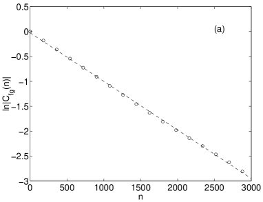
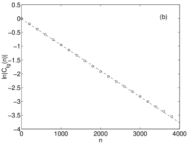
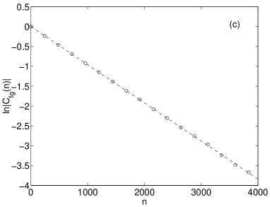
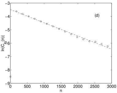
FIG. 1.: The function $C_{fg}(n)$ (semilogarithmic plot) for: (a) $f=g=\phi_{10},K=20,s=370,$ ; (b) $f=g=\phi_{20},K=30,s=900$; (c) $f=g=\phi_{50},K=40,s=3200$; (d) $f=\phi_{12},g=\phi_{13},K=27,s=450$. The dashed line represents the best fit to the data. The number of iterations is $N=8*10^{6}$.

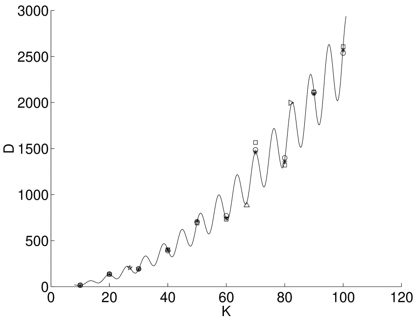
FIG. 2.: The diffusion coefficient $D$ for $K\geq 10$ as found from plots like the ones presented in Fig.1 for: the first mode (1a) (squares), the second mode (1b) (stars), the fifth mode (1c) (circles), correlation function for the off diagonal first mode (1d) (pentagram) and other off diagonal correlation functions (triangles), compared to the theoretical value (solid line).

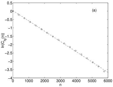
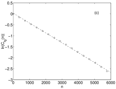
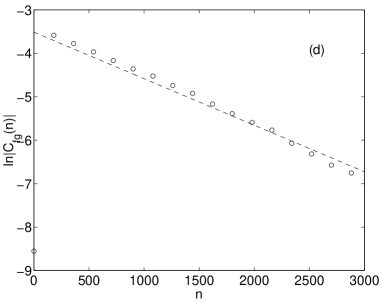
FIG. 3.: The function $C_{fg}(n)$ for (a) $f=g=\phi_{10},K=7,s=250$, (b) $f=g=\phi_{20},K=8,s=510$, (c) $f=g=\phi_{50},K=3,s=340$, (d) $f=\phi_{11},g=\phi_{12},K=17,s=225$. The dashed line represents the best fit to the data. The number of iterations is $N=8*10^{6}$.

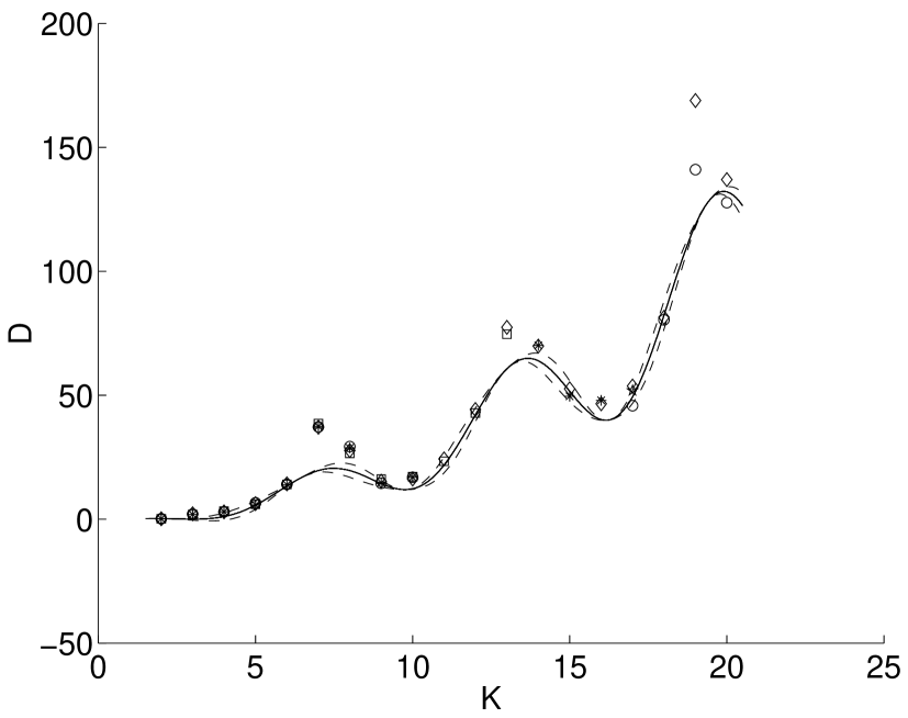
FIG. 4.: The diffusion coefficient $D$ for $K\leq 20$ as found from plots like the ones presented in Fig.3 for: the first mode (1a) (squares) , the second mode (1b) (stars), the fifth mode (1c) (circles) and off diagonal first mode (1d) (pentagram), compared to the theoretical value (solid line). The dashed line represents the approximate error. The values of $D$ obtained by direct simulation of propagation of trajectories are marked by diamonds.

B Angular Relaxation

In order to observe the angular relaxation mode it is required that no relaxation in the $J$ direction is present, because such a relaxation if present, is expected to dominate the long time limit. Since the results are independent on $s$, we use $s=1$. For this purpose we take $g=\phi_{km^{\prime}}$ (see (7)) so that $q=k/s$ is an integer, and $f=\phi_{0m}$. From (69) and (71) one concludes that the slowest of the angular relaxation rates is

$$\tilde{\gamma}=-\frac{1}{2}\ln{[\max_{m^{*}}\left(|J_{2m^{*}}(m^{*}K)|\right)]}.$$ (78)

The absolute value of the correlation function $C_{fg}(n)$ is presented in Figs. 5 and 6 for $g=\phi_{02}$ and $f=\phi_{01}$ and for $g=f=\phi_{01}$ respectively for several values of $K$. The numerical calculations are complicated since the relaxation is fast, with a characteristic time of the order of one time step. Moreover there are oscillations of the correlation function while (78) is just the envelope. In Figs. 5 and 6 the best fit to the envelope is marked by a dashed line. The slope of the dashed line is the numerical estimate for the relaxation rate. In Fig. 7 the numerical estimate is compared with the theoretical prediction. The error in the theoretical prediction is estimated as the value of the next order contribution to $a_{n}$. This results from a term where the “1”s in sequences corresponding to (63) and (65) is replaced by an “$x$” that represents a Bessel function of order $1/\sqrt{K}$, leading to an error of the order $\ln{(1\pm 1/\sqrt{K})}$ in the relaxation rate. It is difficult to estimate the error resulting from the numerical procedure of calculating the relaxation rates. The reason is that near the origin of the correlation function a large number of modes contributes. On the other hand, in the tail of the correlation function, where only one relaxation rate is dominant, the signal is too small. Nevertheless, the comparison between our numerical and theoretical results shows a good qualitative agreement.

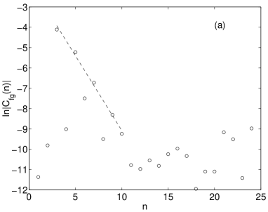
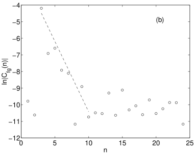
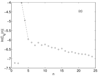
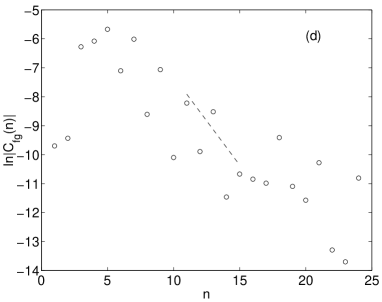
FIG. 5.: The absolute value of the function $C_{fg}(n)$ for $f=\phi_{01},g=\phi_{02}$ and (a) K=16.3, (b) K=19.5, (c) K=12, (d) K=16. The dashed line represents the best fit to the data. The values $s=1$ and $N=10^{8}$ were used.

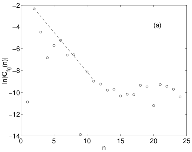
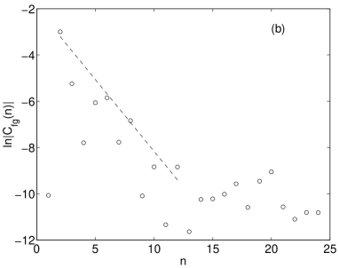
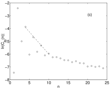
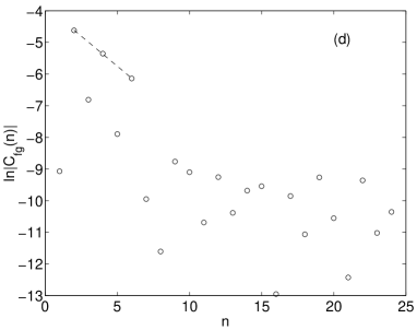
FIG. 6.: The absolute value of the function $C_{fg}(n)$ for $f=g=\phi_{01}$ and (a) K=10.7, (b) K=14.3, (c) K=12.55, (d) K=14.7. The dashed line represents the best fit to the data. The values $s=1$ and $N=10^{8}$ were used.

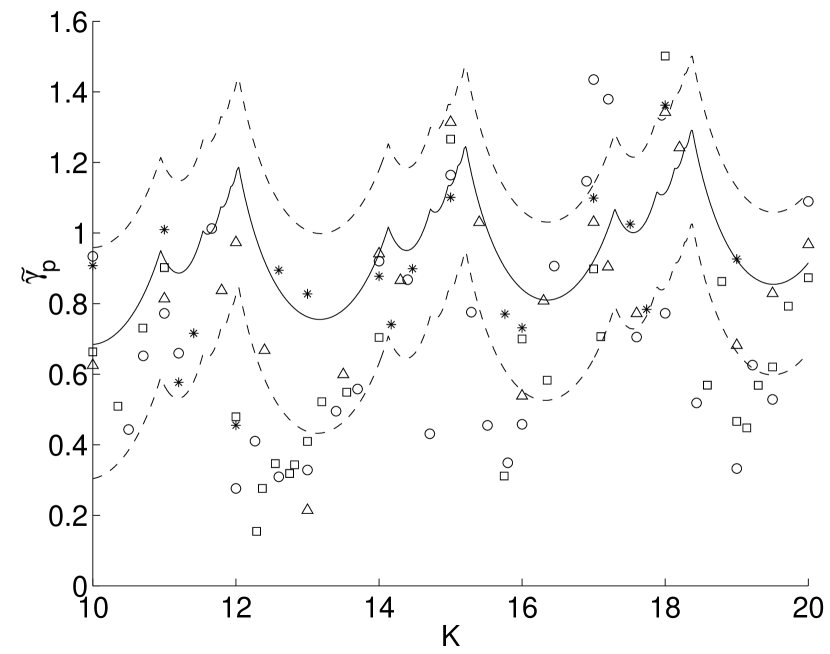
FIG. 7.: The fast relaxation rate $\tilde{\gamma}$ as found from plots like Figs. 5 and 6 for $f=\phi_{01}$, $g=\phi_{02}$(triangles), $f=\phi_{02}$, $g=\phi_{04}$(circles), $f=g=\phi_{02}$(stars) and $f=g=\phi_{01}$(squares), compared to the theoretical value (78) (solid line). The dashed lines denote the theoretically estimated error. Here we used $s=1$ and $N=10^{8}$.

V Summary and Discussion

Relaxation to equilibrium was studied for the kicked rotor that is a standard system for the exploration of classical chaos in driven systems and its quantum mechanical suppression. Relaxation and diffusion are important concepts in statistical mechanics. Here they were studied for a mixed chaotic system. Very little is known rigorously about such systems although most models describing real physical systems are mixed, namely in some regions of phase space the motion is regular while in some regions it is chaotic.

In this work the kicked rotor was studied in a phase space that is the torus defined by (6). The relaxation of distributions in phase space takes place in stages. First, the inhomogeneity in $\theta$ decays with rapid relaxation rates, the slowest of them is $\tilde{\gamma}$. Then relaxation of the inhomogeneities in the $J$ direction takes place with the relaxation rates related to the diffusion coefficient via (77). Diffusion was previously believed to be a good approximation for the kicked rotor, but here, to our best knowledge, the various time scales were analyzed carefully for the first time. In particular we have found the time scale, $1/\tilde{\gamma}$, below which the diffusion approximation does not hold since relaxation of correlations in the angle direction still takes place.

There is a clear relation between the relaxation of inhomogeneities in $\theta$ and the diffusion constant since

$$<(J_{n+1}-J_{0})^{2}>=\sum_{i,j=0}^{n}K^{2}<sin\theta_{i}sin\theta_{j}>,$$ (79)

where $J_{i}$ and $\theta_{i}$ are the momentum and angle before the $i$-th kick. For a chaotic trajectory

$$<sin\theta_{i}sin\theta_{j}>=<sin\theta_{0}sin\theta_{|i-j|}>=C_{ff}(|i-j|),$$ (80)

where $C_{ff}(|i-j|)$ is the correlation function (74) with $f=\phi_{01}$. If the sum $\sum_{i=0}^{\infty}C_{ff}(i)$ converges, as is the case where $C_{ff}$ falls off exponentially, diffusion is found and the value of the diffusion coefficient is

$$D=\frac{K^{2}}{2}\sum_{i=-\infty}^{\infty}C_{ff}(i).$$ (81)

In App. C we show that (50) that was obtained by Rechester and White in  [14] is just

$$D=\frac{K^{2}}{2}\sum_{i=-2}^{2}C_{ff}(i).$$ (82)

A derivation that is very similar is presented in  [28]. If the sum diverges one obtains anomalous diffusion.

Finite noise leads to the effective truncation of the evolution operator (21) . In the basis (7) it means that it results in limited resolution. Moreover for $\sigma>0$ the operator $\tilde{U}$ is nonunitary. The approximate eigenvalues of $\hat{U}$ given by (21), that were found in this work are $1$ and $z_{k}$ of (48) ( if (40) satisfied ) and $\tilde{z}$ of (71). In our approximation method we could not obtain many eigenvalues related to angular relaxation modes. Because of the effective truncation, $\psi_{\gamma}$, the eigenfunction of $\hat{U}$, can be expanded in terms of the basis states (7). The relaxation rates of these states are $-ln(z_{k})$ and $-ln(|\tilde{z}|)$, where $z_{k}$ and $\tilde{z}$ are given by (48) and (71). In the limit $\sigma\rightarrow 0$ the evolution operator is unitary, $\psi_{\gamma}$ approach some generalized functions while $z_{k}$ and $\tilde{z}$ approach the values of the poles of the matrix elements of the resolvent $\hat{R}$ of (25) obtained from the extrapolation from $|z|>1$ (corresponding to the $0<\epsilon\rightarrow 0$, used in the standard definition of the Green’s function ).

These are the Ruelle resonances that are related to the relaxation rates via (70) and (71). This is very similar to the situation for hyperbolic systems such as the baker map. For hyperbolic systems the Ruelle resonances ( related to the relaxation rates ) approach fixed values inside the unit circle in the complex $z$ plane in the limit of an infinite matrix for the evolution operator or of infinitely fine phase space resolution. This was found to be correct also here when one takes the limit $\sigma\rightarrow 0$ in (49) and (66) resulting in (68) and (69). Numerical tests in absence of noise confirm that the analytical results provide a good approximation for the relaxation to equilibrium and diffusion in the chaotic component. Results of similar nature were found in the standard map with $s=1$ for some values of $K$ [19], for the “perturbed cat” map [19], and also for the kicked top [20]. In all these works it was found, within the approximations used, that the leading resonances are either real or form the quartet $(\pm A,\pm iA)$ where $A$ is a real number satisfying $0<A<1$. The generality of this form should be subject to further research. For the kicked top it was attributed [20] to the dominance of an orbit of period $4$.

In mixed systems, such as the kicked rotor, even in the chaotic components there is sticking to regular islands and acceleration modes. Noise eliminates this sticking . The analytic formulas (68) and (69) are obtained from an expansion in powers of $1/\sqrt{K}$ for finite variance of noise $\sigma^{2}$ and the limit $\sigma^{2}\rightarrow 0$ is taken in the end of the calculation. A nonvanishing value of $\sigma^{2}$ assures the convergence of the series (57). Appearance of the islands and the sticking is a nonperturbative effect and therefore it is not reproduced in our theory. For this reason in absence of noise the results are only approximate. The effect of the sticking is extremely small for most values of the stochasticity parameter $K$, as verified by the numerical calculations without noise.

The physical reason for the decay of correlations is, that in a chaotic system, because of the stretching and folding mechanisms there is persistent flow in the direction of functions with finer details namely larger $|k|$ and $|m|$ in our case. Consequently the projection on a given function, for example one of the basis functions (7) in our case, decays  [20, 29]. The crucial point is that this function should be sufficiently smooth. This argument should hold also for the chaotic component of mixed systems. In the present paper the actual relaxation rates were calculated. Here noise was used in order to make the analytical calculations possible. In real experiments some level of noise is present, therefore the results in presence of noise are of experimental relevance. It was shown with the help of the Cauchy-Hadamard theorem  [27] ( see discussion following (32) ) that for $s>>K>>1$ exponential relaxation to the invariant density takes place with the rate $\gamma_{1}=D(K)/s^{2}$, where $D(K)$ is given by (4). It was deduced from the radius of convergence for the series of the matrix element of $\hat{R^{\prime}}$ (see (29)). This rate is independent of $\sigma$. It is found for all functions that can be expanded in the basis (7), with an absolutely convergent expansion. It excludes for example functions of the form (22). We believe this statement can be made rigorous by experts.

For the baker map it was found that the resolvent of the evolution operator of the Quantum Wigner function, when coarse grained has the same poles as the classical Frobenius-Perron operator  [21]. We believe it should hold also here. The fact that the Ruelle resonances of the modes of slow relaxation are $z_{k}$ that are identical to the ones of the diffusion operator gives additional support to approximations made for the calculation of the ensemble averaged localization length in  [24].

Finally, the Ruelle resonances, that were introduced and established rigorously for hyperbolic systems can be used to describe relaxation and transport in the chaotic component of mixed systems. Here it was demonstrated for the kicked-rotor.

VI Acknowledgments

We have benefited from discussions with E. Berg, R. Dorfman, I. Guarneri, F. Haake, E. Ott, R. Prange, S. Rahav, J. Weber and M. Zirenbauer. We thank in particular D. Alonso for extremely illuminating remarks and helpful suggestions. This research was supported in part by the US–NSF grant NSF DMR 962 4559, the U.S.–Israel Binational Science Foundation (BSF), by the Minerva Center for Non-linear Physics of Complex Systems, by the Israel Science Foundation, by the Niedersachsen Ministry of Science (Germany) and by the Fund for Promotion of Research at the Technion. One of us (SF) would like to thank R.E. Prange for the hospitality at the University of Maryland where this work was completed.

A The matrix elements of the evolution operator in presence of noise.

In this appendix the matrix elements in the representation (7) are calculated. For this purpose (20) is transformed to the Fourier representation by

$$(k_{2}m_{2}|\hat{U}|k_{1}m_{1})=\int_{0}^{2\pi}d\theta\int_{0}^{2\pi s}dJ\int_{0}^{2\pi}d\theta^{\prime}\int_{0}^{2\pi s}dJ^{\prime}(k_{2}m_{2}|J\theta)(J\theta|\hat{U}_{noise}|J^{\prime}\theta^{\prime})(J^{\prime}\theta^{\prime}|\hat{U}_{K}|k_{1}m_{1}).$$ (A1)

Substitution of (18) and (19) yields

$$(k_{2}m_{2}|\hat{U}|k_{1}m_{1})=\int_{0}^{2\pi}d\theta\int_{0}^{2\pi s}dJ\int_{0}^{2\pi}d\theta^{\prime}\frac{1}{\sqrt{2\pi}}\frac{1}{\sqrt{2\pi s}}\exp(-im_{2}\theta)\exp\left(i\frac{-k_{2}J}{s}\right)$$ (A2)

$\displaystyle\sum_{m}\frac{1}{2\pi}\exp(im(\theta^{\prime}-\theta))\exp\left(-imJ-\frac{\sigma^{2}}{2}m^{2}\right)\frac{1}{\sqrt{2\pi}}\frac{1}{\sqrt{2\pi s}}\exp(im_{1}\theta^{\prime})\exp\left(i\frac{k_{1}}{s}(J+Ksin\theta^{\prime})\right).$

Terms containing $\theta$ are $\exp(im(-\theta))\exp(-im_{2}\theta)$. Integration over $\theta$ yields $\delta_{m,-m_{2}}$ leading to

$$(k_{2}m_{2}|\hat{U}|k_{1}m_{1})=\int_{0}^{2\pi s}dJ\int_{0}^{2\pi}d\theta^{\prime}\frac{1}{\sqrt{2\pi s}}\exp\left(i\frac{-k_{2}J}{s}\right)$$ (A3)

$\displaystyle\frac{1}{2\pi}\exp(i(-m_{2}\theta^{\prime})\exp\left(im_{2}J-\frac{\sigma^{2}}{2}m_{2}^{2}\right)\frac{1}{\sqrt{2\pi s}}\exp(im_{1}\theta^{\prime})\exp\left(i\frac{k_{1}}{s}(J+Ksin\theta^{\prime})\right).$

Integration over $J$ results in $\delta_{k_{2}-k_{1},m_{2}s}$, yielding

$$(k_{2}m_{2}|\hat{U}|k_{1}m_{1})=\frac{1}{2\pi}\int_{0}^{2\pi}d\theta^{\prime}\exp(-i(m_{2}-m_{1})\theta^{\prime})\exp\left(-\frac{\sigma^{2}}{2}m_{2}^{2}\right)\exp\left(i\frac{k_{1}}{s}Ksin\theta^{\prime}\right)\delta_{k_{2}-k_{1},m_{2}s}$$ (A4)

Finally with the help of the integral representation for Bessel functions:

$\displaystyle J_{m}(z)=\frac{1}{2\pi}\int_{0}^{2\pi}d\theta\exp(-im\theta)\exp(izsin\theta)$

one obtains (21).

B The end terms in strings of the fast modes

In this appendix, possible examples for contributions to the end terms in (65) are presented. The left end term is a sum of terms of the form

$$C^{(l)}(m,m^{*})=$$ (B2)

$$J_{2m+m^{*}}(-mK)~{}J_{-m-2m^{*}}(m^{*}K)~{}J_{0}(0)~{}\exp\left[-\frac{\sigma^{2}}{2}\left(m^{2}+(m+m^{*})^{2}+m^{*2}\right)\right]$$

$$+ \sum_{m_{1}}J_{m-m_{1}}(-mK)~{}J_{2m_{1}+m+m^{*}}((-m-m_{1})K)~{}J_{-m-2m^{*}-m_{1}}(m^{*}K)~{}J_{0}(0)~{}$$ (B4)

$$\exp\left[-\frac{\sigma^{2}}{2}\left(m^{2}+m_{1}^{2}+(m+m^{*}+m_{1})^{2}+m^{*2}\right)\right]...$$

where in the first term $m_{1}=(m+m^{*})$ and $m_{2}=m_{3}=m^{*}$ while in the second term $m_{2}=-(m+m^{*}+m_{1})$ and $m_{3}=m_{4}=m^{*}$. For $q\neq 0$ the right end term is a sum of terms of the form

$$C^{(r)}(m^{*},m^{\prime},q)=$$ (B5)

$$\sum_{m_{n-1}}J_{2m^{*}+m_{n-1}+q}(-m^{*}K)~{}J_{-m^{*}-2m_{n-1}-q}((m_{n-1}+q)K)~{}J_{m_{n-1}-m^{\prime}}(qK)$$ (B6)

$$~{}\exp\left[-\frac{\sigma^{2}}{2}\left(m^{*2}+(m^{*}+m_{n-1}+q)^{2}++m_{n-1}^{2}\right)\right]....$$ (B7)

where $m_{n-2}=-(m^{*}+m_{n-1}+q)$ and $m_{n-3}=m^{*}$. For $q=0$ one has to take $m_{n-1}=m^{\prime}$ and the end term consists of a sum over $m_{n-2}$.

C The relation between the diffusion coefficient and correlation function.

In this appendix the relation between (82) and (50) will be derived ( for a somewhat similar derivation see  [28] ). For this purpose we note that

$$C_{ff}(n)=\int_{0}^{2\pi}\frac{d\theta}{2\pi}\int_{0}^{2\pi s}\frac{dJ}{2\pi s}sin\theta\ \hat{U^{n}}\ sin\theta=-\frac{1}{4}[(0,-1|-(0,1|]\hat{U^{n}}[|0,1)-|0,-1)],$$ (C1)

where the representation $|k,m)$ (see (7)) is used. The matrix elements of $\hat{U}$ are given by (21) and the matrix elements of $\hat{U^{2}}$ required for the present calculation are

$$(0,m_{2}|\hat{U^{2}}|0,m_{1})=J_{2m_{2}}\left(-m_{2}K\right)e^{-\sigma^{2}m_{2}^{2}}\delta_{m_{1},-m_{2}}$$ (C2)

as can be easily obtained from multiplication of two matrices of the form (21). From (C1) it is clear that $C_{ff}(0)=\frac{1}{2}$. Inspecting (21) with $k_{1}=k_{2}=0$ one notes that it is required that also $m_{1}=m_{2}=0$, therefore $C_{ff}(1)=0$. Substitution of (C2) in (C1) yields

$$C_{ff}(2)=-\frac{1}{2}J_{2}\left(K\right)e^{-\sigma^{2}}.$$ (C3)

Using the fact that $C_{ff}(-n)=C_{ff}(n)$, substitution of the values of $C_{ff}(0)$ and $C_{ff}(2)$ into (82) yields the expression (50) that was obtained by Rechester and White  [14]. Because of the discussion following (59) the correlation functions $C_{ff}(n)$ with $n>2$ lead to terms that are of higher orders in $1/\sqrt{K}$ than (50).

REFERENCES

- [1] E. Ott, Chaos in Dynamical Systems, Cambridge University Press, Cambridge, (1997).
- [2] V.I. Arnold and A. Avez, Ergodic Problems of Classical Mechanics, (Addison-Wesley NY, 1989).
- [3] P. Gaspard, Chaos, Scattering and Statistical Mechanics, (Cambridge Press, Cambridge 1998).
- [4] J.R. Dorfman, An Introduction to Chaos in Non-Equilibrium Statistical Mechanics, (Cambridge Press, Cambridge 1999).
- [5] D. Ruelle, Statistical Mechanics, Thermodynamic Formalism, (Addison-Wesley, Reading MA,1978); D. Ruelle, Phys. Rev. Lett. 56, 405 (1986).
- [6] P. Cvitanovi and B. Eckhardt, J. Phys. A 24, L237 (1991).
- [7] P. Gaspard, Phys. Rev. E 53, 4379 (1996).
- [8] A.J. Lichtenberg and M.A. Lieberman, Regular and Stochastic Motion (Springer, NY 1983).
- [9] B.V. Chirikov, Phys. Repts. 52, 263 (1979).
- [10] R. Balescu ,Statistical Dynamics, Matter out of Equilibrium, (Imperial College Press ,Singapore, 1983).
- [11] G. Casati, B.V. Chirikov, F.M. Izrailev and J. Ford in Stochastic Behavior in Classical and Quantum Hamiltonian systems, Vol. 93 of Lecture Notes in Physics, edited by G. Casati and J. Ford (Springer, Berlin 1979), p. 334
- [12] S. Fishman, D.R. Grempel and R.E. Prange, Phys. Rev. Lett. 49, 509 (1982); D.R. Grempel, R.E. Prange and S. Fishman, Phys. Rev. A29, 1639 (1984).
- [13] S. Fishman Quantum Localization, Lecture notes for the 44th Scottish Universities Summer School in Physics on Quantum Dynamics of Simple Systems Stirling, Scotland , 15-26 August 1994.
- [14] A.B. Rechester and R.B. White, Phys. Rev. Lett. 44, 1586 (1980); A.B. Rechester M.N. Rosenbluth and R.B. White, Phys. Rev. A 23, 2664 (1981); E. Doron and S. Fishman, Phys. Rev. A 37, 2144 (1988).
- [15] S. Benkadda, S. Kassibrakis, R.B. White and G.M. Zaslavsky, Phys. Rev. E 55, 4909 (1997); G.M. Zaslavsky, J. Plasma Physics. 59, part 4, 671 (1998); G.M. Zaslavsky, B.A. Niyazov, Phys. Repts. 283, 73 (1979); B. Sundaram and G.M. Zaslavsky, Phys. Rev. E59, 7231 (1999); G.M. Zaslavsky, M. Edelman and B.A. Niyazov, Chaos 7, 1 (1997).
- [16] A short version of this work is presented in M. Khodas and S. Fishman, Phys. Rev. Lett. 84, 2837 (2000).
- [17] H.H. Hasegawa and W.C. Saphir, Phys. Rev. A 46, 7401 (1992).
- [18] I. Antoniou, B. Qiao, Z. Suchanecki, Chaos Solitons & Fractals 8, 77 (1997).
- [19] G. Blum and O. Agam, to be published in Phys. Rev E.
- [20] J. Weber, F. Haake and P. Šeba, Frobinius-Perron Resonances for Maps with a Mixed Phase Space, CD/0001013 and private communications.
- [21] S.Fishman, in Suppersymmetry and Trace Formulae, Chaos and Disorder, edited by I.V. Lerner, J.P. Keating, D.E. Khmelnitskii (Kluwer Academic / Plenum Publishers, New York, 1999).
- [22] M.R. Zirnbauer, in Suppersymmetry and Trace Formulae, Chaos and Disorder, edited by I.V. Lerner, J.P. Keating, D.E. Khmelnitskii (Kluwer Academic / Plenum Publishers, New York, 1999), p. 193.
- [23] A. V. Andreev and B. L. Altshuler, Phys. Rev. Lett. 75, 902 (1995); O. Agam, B. L. Altshuler, and A. V. Andreev, Phys. Rev. Lett. 75, 4389 (1995); A. V. Andreev, O. Agam, B. D. Simons and B. L. Altshuler, Phys. Rev. Lett. 76, 3947 (1996); Nuclear Physics B482, 536 (1996); Phys. Rev. Lett. 79, 1778 (1997); O. Agam, A. V. Andreev, and B. D. Simons, Chaos, Solitons & Fractals 8, 1099 (1997); J. Math. Phys. 38, 1982 (1997).
- [24] A. Altland and M. R. Zirnbauer, Phys. Rev. Lett. 77, 4536 (1996); 80, 641 (1998).
- [25] G. Casati, F. M. Israilev and V. V. Sokolov, Phys. Rev. Lett. 80, 640 (1998).
- [26] M. V. Berry, in New trends in Nuclear Collective Dynamics, eds: Y. Abe, H. Horiuchi, K. Matsuyanagi, Springer proceedings in Physics. vol 58 pp183-186 (1992).
- [27] K. Knopp, Infinite Sequences and Series, (Dover publ. NY, 1956).
- [28] Cary, J. R., J. D. Meiss, A. Bhattacharee, Phys. Rev. A23, 2744 (1981).
- [29] F. Haake, Lecture at the International Workshop and Seminar on Dynamics of Complex Systems, Dresden, May, 1999.