Escape Probability and Mean Residence Time in Random Flows with Unsteady Drift

Abstract

We investigate fluid transport in random velocity fields with unsteady drift. First, we propose to quantify fluid transport between flow regimes of different characteristic motion, by escape probability and mean residence time. We then develop numerical algorithms to solve for escape probability and mean residence time, which are described by backward Fokker-Planck type partial differential equations. A few computational issues are also discussed. Finally, we apply these ideas and numerical algorithms to a tidal flow model.

Key Words: Random velocity fields, fluid transport, escape probability, mean residence time, finite element method and tidal flow

Short Running Title: Transport in Random Flows

1 Introduction

The Lagrangian view of fluid motion is particularly important in geophysical flows since only Lagrangian data can be obtained in many situations. It is essential to understand fluid particle trajectories in many fluid problems.

Stochastic dynamical systems arise as models for fluid particle motion in geophysical flows with random velocity field

$$\dot{x} = f(x,y,t)+a(x,y)\dot{w}_{1},$$ (1)

$$\dot{y} = g(x,y,t)+b(x,y)\dot{w}_{2},$$ (2)

where $w_{1}(t),w_{2}(t)$ are two real independent Brownian motion processes, $f,g$ are deterministic drift part, and $a,b$ are the intensity coefficients of diffusive noise part, of the velocity field. Note that the generalized derivative of a Brownian motion process is a mathematical model for “white noise”. For general background in stochastic dynamical systems, see [1, 6, 9].

Deterministic quantities, such as escape probability (from a fluid domain) and mean residence time (in a fluid domain), that characterize stochastic dynamics can be computed by solving the Fokker-Planck type backward partial differential equations.

In a previous paper [3], when the drift is steady, i.e, $f,g$ do not depend on time, we have quantified fluid transport between flow regimes of different characteristic motion by escape probability and mean residence time; developed methods for computing escape probability and mean exit time; and applied these methods in the investigation of geophysical fluid dynamics. In this paper, we further consider the case of unsteady or nonautonomous drift $f(x,y,t),g(x,y,t)$, develop a numerical algorithm for computing escape probability and mean exit time, and demonstrate the application of this approach to a tidal flow model.

2 Stochastic Dynamics
of Fluid Particle Motion

For a planar bounded domain $D$, we can consider the exit problem of random solution trajectories of (1)-(2) from $D$. To this end, let $\partial D$ denote the boundary of $D$. The residence time of a particle initially at $(x,y)$ at time $t$ inside $D$ is the time until the particle first hits $\partial D$ (or escapes from $D$). The mean residence time $\tau(x,y,t)=t+u(x,y,t)$, where $u(x,y,t)$ satisfies [8]

$$u_{t}+\frac{1}{2}a^{2}u_{xx}+\frac{1}{2}b^{2}u_{yy} + f(x,y,t)u_{x}+g(x,y,t)u_{y}=-1,$$ (3)

$$u(x,y,t) = 0,\;(x,y,t)\in\partial D\times(0,T),$$ (4)

$$u(x,y,T) = 0,\;(x,y)\in D,$$ (5)

where $T$ is big enough, i.e., $T>\sup\tau(x,y,t)$ and here the $\sup$ is taken over all $(x,y)$ in a compact set, i.e., the closure of the domain $D$.

Note that $u(x,y,t)=\tau(x,y,t)-t$ is the mean residence time after time instant $t$, or it quantifies how much longer a particle will stay inside $D$ after we observe it at position $(x,y)$ at the time instant $t$.

Let $\Gamma$ be a part of the boundary $\partial D$. The escape probability $p(x,y,t)$ is the probability that the trajectory of a particle starting at position $(x,y)$ and at instant $t$ in $D$ first hits $\partial D$ (or escapes from $D$) at some point in $\Gamma$ (prior to escape through $\partial D-\Gamma$), and $p(x,y,t)$ satisfies [10, 15]

$$p_{t}+\frac{1}{2}a^{2}p_{xx}+\frac{1}{2}b^{2}p_{yy} + f(x,y,t)p_{x}+g(x,y,t)p_{y}=0,$$ (6)

$$p(x,y,t) = 0,\;(x,y,t)\in(\partial D-\Gamma)\times(0,T),$$ (7)

$$p(x,y,t) = 1,\;(x,y,t)\in\Gamma\times(0,T),$$ (8)

$$p(x,y,T) = 1,\;(x,y)\in D.$$ (9)

Note that $p(x,y,t)$ depends on $\Gamma$, and it may be better denoted as $p_{\Gamma}(x,y,t)$.

Suppose that initial conditions (or initial particles) are uniformly distributed over $D$. The average escape probability $P(t)$ that a trajectory will leave $D$ along the subboundary $\Gamma$ at time $t$, before leaving the rest of the boundary, is given by [10]

$$P(t)=\frac{1}{|D|}\int\int_{D}p(x,y,t)dxdy,$$ (10)

where $|D|$ is the area of domain $D$.

3 Numerical Approaches

For the backward type of partial differential equation (3), we reverse the time

$$s=T-t$$

Then the mean residence time $u(x,y,s)$ (we still use the same notation) satisfies

$$u_{s} = \frac{1}{2}a^{2}u_{xx}+\frac{1}{2}b^{2}u_{yy}$$ (11)

$$+ f(x,y,T-s)u_{x}+g(x,y,T-s)u_{y}+1,$$

$$u(x,y,s) = 0,\;(x,y,s)\in\partial D\times(0,T),$$ (12)

$$u(x,y,0) = 0,\;(x,y)\in D.$$ (13)

Similarly for the escape probability $p(x,y,s)$ (we still use the same notation), we have

$$p_{s} = \frac{1}{2}a^{2}p_{xx}+\frac{1}{2}b^{2}p_{yy}+f(x,y,T-s)p_{x}+g(x,y,T-s)p_{y},$$ (14)

$$p(x,y,s) = 0,\;(x,y,s)\in(\partial D-\Gamma)\times(0,T),$$ (15)

$$p(x,y,s) = 1,\;(x,y,s)\in\Gamma\times(0,T),$$ (16)

$$p(x,y,0) = 1,\;(x,y)\in D.$$ (17)

A piecewise linear, finite element approximation scheme [4] was used for the numerical solutions of the escape probability $p(x,y,s)$, and the mean residence time $u(x,y,s)$, described by the parabolic equations (11), and (14), respectively. By transforming back to original time $t=T-s$, we get $p(x,y,t)$, and $u(x,y,t)$. We have used a few different time-discretization schemes, including the implicit backward in time, and Crank-Nicholson scheme [5]. The code works also for boundary defined by a collection of points lying on the boundary. A piecewise cubic splines were constructed to define such boundaries.

4 Application to a Tidal Flow

To demonstrate the above ideas and numerical algorithms, we consider a tidal flow model. This flow model is very idealistic and here we just use it as an illuminating example.

Oscillatory tidal water motions dominate a large part of the coastal regions. Beerens and Zimmerman [2] considered a tidal flow model with velocity field

$$u_{o} = \pi\sin(\pi x)\cos(\pi y)+\pi\lambda\cos(2\pi t),$$ (18)

$$v_{o} = -\pi\cos(\pi x)\sin(\pi y),$$ (19)

where $\lambda$ is a parameter measuring the intensity of the tidal wave $\pi\cos(2\pi t)$. We take $0<\lambda<3$ as used by Beerens and Zimmerman [2].

As pointed out by Beerens and Zimmerman [2], it is essential to include more complicated temporal modes in this model in order to describe more realistic tidal flows. We include random temporal modes or white noise in this model, i.e., we consider a tidal flow model with unsteady drift part and random diffusive part:

$$\hat{u}_{o} = \pi\sin(\pi x)\cos(\pi y)+\pi\lambda\cos(2\pi t)+\sqrt{2\epsilon}\dot{w}_{1},$$ (20)

$$\hat{v}_{o} = -\pi\cos(\pi x)\sin(\pi y)+\sqrt{2\epsilon}\dot{w}_{2},$$ (21)

where $\epsilon>0$ is the constant intensity of the white noise. We assume that the random temporal modes are weaker than the time-periodic mode and so we take $0<\epsilon<0.1$ in the following simulations.

We study the transport of fluid particles in this tidal flow model. The equations of motion of fluid particles in this tidal flow are

$$\dot{x} = \pi\sin(\pi x)\cos(\pi y)+\pi\lambda\cos(2\pi t)+\sqrt{2\epsilon}\dot{w}_{1},$$ (22)

$$\dot{y} = -\pi\cos(\pi x)\sin(\pi y)+\sqrt{2\epsilon}\dot{w}_{2},$$ (23)

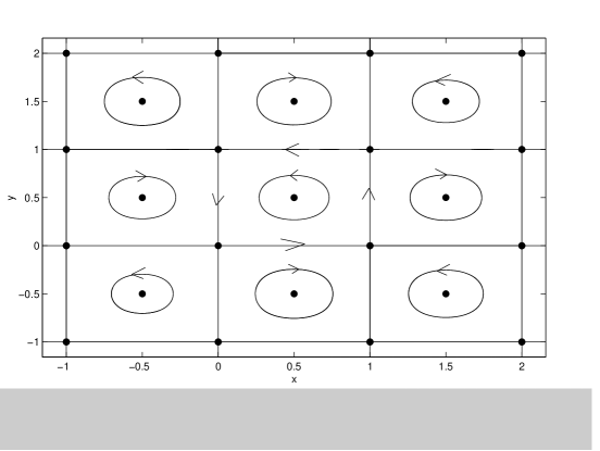
where $w_{1}(t),w_{2}(t)$ are two independent Brownian motion processes. The unperturbed flow, with no temporal periodic “tidal” mode $\cos(2\pi t)$ and no temporal white noise modes $\dot{w}_{1},\dot{w}_{2}$ of this tidal flow model, is the so-called cellular flow:

$$\dot{x} = \pi\sin(\pi x)\cos(\pi y),$$ (24)

$$\dot{y} = -\pi\cos(\pi x)\sin(\pi y).$$ (25)

Figure 1 shows the phase portrait of this unperturbed flow (24)-(25).

Figure 1: Unperturbed flow

The partial differential equations for mean residence time $u$ of fluid particles in a fluid domain $D$, and for the escape probability $p$ of fluid particles cross a subboundary $\Gamma$ of $D$, are the following (in reversed time $s=T-t$), respectively,

$$u_{s} = \epsilon(u_{xx}+u_{yy})$$ (26)

$$+ [\pi\sin(\pi x)\cos(\pi y)+\pi\lambda\cos(2\pi T-s)]u_{x}$$

$$- \pi\cos(\pi x)\sin(\pi y)u_{y}+1,$$

$$p_{s} = \epsilon(p_{xx}+p_{yy})$$ (27)

$$+ [\pi\sin(\pi x)\cos(\pi y)+\pi\lambda\cos(2\pi T-s)]p_{x}$$

$$- \pi\cos(\pi x)\sin(\pi y)p_{y}.$$

In practical numerical simulations, the “final” time $T$ should be taken big enough so that the solutions $u$, $p$ do not change within a reasonable tolerance. To do so, we monitor the mean-square difference of $u$ (and also $p$) at time $T$ and $T+1$. When this difference is within a reasonable tolerance (we use $0.001$), we take the $T$ as the “final” time; otherwise, we increase the value of $T$ and do the simulation again, until the tolerance criterion is met.

We take a fluid domain $D$ to be a typical cell, i.e., the unit square, in the unperturbed flow; see Figure 2.

Figure 2: A fluid domain $D$

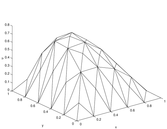
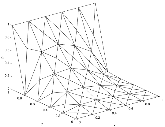
Unlike the stochastic systems with steady drift as studied by Brannan, Duan and Ervin [3], the mean residence time and escape probability depend on time (although the change is small in this specific example); see Figures 3, 4, 5 and 6. All these plots are for $\lambda=1$ and $\epsilon=0.1$. The mean residence time and escape probability for $0<\lambda<3$ and $0<\epsilon<0.1$ display similar features.

Figure 3: Mean residence time after time $t=10$

Figure 4: Mean residence time after time $t=50.5$

Figure 5: Escape probability crossing the top boundary $y=1$ after time $t=10$

Figure 6: Escape probability crossing the top boundary $y=1$ after time $t=60$

In this flow model, it turns out that the average escape probability crossing the top boundary $y=1$ does not change much with time, with value around $0.2639$. We observe similar features for crossing other three side boundaries.

In the tidal flow model (18)-(19) with only time-periodic “tidal” mode $\pi\lambda\cos(2\pi t)$, Beerens and Zimmerman [2] found that there are “islands” in the tidal flow and the fluid particles trapped in such islands will never escape, for $0<\lambda<3$ as used by Beerens and Zimmerman [2]. This phenomenon is common in non-dissipative, Hamiltonian planar systems. Although the dissipation in the oceans is small, “no matter how small the dissipation is, the (oceanic) fluid has substantial time to experience the action of dissipative forces” [12]. So this “islands” phenomenon does not appear to be likely in realistic tidal flows; see more physical discussions in [7, 11, 14].

While in our tidal flow model (20)-(21) with both time-periodic “tidal” mode $\pi\lambda\cos(2\pi t)$ and temporal white noise modes, all fluid particles will eventually escape from any fluid domain in finite time after we first observe them; see Figures 3, 4. This feature is true for any $\epsilon>0$. It appears that our stochastic tidal model is a little more realistic than Beerens and Zimmerman’s model [2]. We remark again that we use this simple tidal flow model to demonstrate the applications of mean residence time and escape probability.

In summary, in this paper we have discussed the quantification of fluid transport between flow regimes of different characteristic motion by escape probability and mean residence time, developed numerical algorithms to solve for escape probability and mean residence time, and applied these ideas and numerical algorithms to a tidal flow model.

Acknowledgement.

We would like to thank Ludwig Arnold for very useful suggestions. We would also thank the hospitality of the Oberwolfach Mathematical Research Institute, Germany. This work was supported by the NSF Grant DMS-9704345.

References

- [1] L. Arnold, Random Dynamical Systems, Springer-Verlag, New York, 1998.
- [2] S. P. Beerens, H. Ridderinkhof and J. T. F. Zimmerman, An analytical study of chaotic stirring in tidal areas, Chaos, Solitons and Fractals 4 (1994), 1011-1029.
- [3] J. Brannan, J. Duan and V. Ervin, Escape Probability, Mean Residence Time and Geophysical Fluid Particle Dynamics, Physica D 133 (1999).
- [4] S. Brenner and L. Scott, The Mathematical Theory of Finite Element Methods, Springer-Verlag, New York, 1996.
- [5] K. Eriksson, D. Estep, P. Hansbo and C. Johnson, Computational Differential Equations, Cambridge, Sweden, 1996.
- [6] M. I. Freidlin and A. D. Wentzell, Random Perturbations of Dynamical Systems, Springer-Verlag, New York, 1984.
- [7] A. E. Gill, Atmosphere-Ocean Dynamics, Academic Press, New York, 1982.
- [8] R. Z. Hasminskii, Stochastic Stability of Differential Equations, Sijthoff & Noordhoff, The Netherlands, 1980.
- [9] B. Oksendal, Stochastic Differential Equations: An Introduction with Applications, Springer-Verlag, New York, 5th ed., 1998.
- [10] C. C. Lin and L. A. Segel, Mathematics Applied to Deterministic Problems in the Natural Sciences, SIAM, Philadelphia, 1988.
- [11] J. Pedlosky, Geophysical Fluid Dynamics, Springer-Verlag, 2nd edition, 1987.
- [12] J. Pedlosky, Ocean Circulation Theory, Springer-Verlag, 1996.
- [13] H. Risken, The Fokker-Planck Equation, Springer-Verlag, 1984.
- [14] R. Salmon, Lectures on Geophysical Fluid Dynamics, Oxford Univ. Press, Oxford, 1998.
- [15] Z. Schuss, Theory and Applications of Stochastic Differential Equations, Wiley Sons, 1980.