Detecting and analysing nonstationarity in a time series with nonlinear cross–predictions

Abstract

We propose an informal test for stationarity in a time series which checks for the compatibility of nonlinear approximations to the dynamics made in different segments of the sequence. The segments are compared directly, rather than via statistical parameters. The approach provides detailed information about episodes with similar dynamics during the measurement period. Thus physically relevant changes in the dynamics can be followed.
PACS: 05.45.+b

Almost all methods of time series analysis, traditional linear or nonlinear, must assume some kind of stationarity. Therefore, changes in the dynamics during the measurement period usually constitute an undesired complication of the analysis. There are however situations where such changes represent the most interesting structure in the recording. For example, electroencephalographic (EEG) recordings are often taken with the main purpose of identifying changes in the dynamical state of the brain. Such changes occur e.g. between different sleep stages, or between epileptic seizures and normal brain activity. In this letter we propose an approach to the study of potentially nonstationary signals which does not only provide a powerful test for stationarity but also allows for a time resolved study of the dynamical changes. While testing for stationarity might appear to be a technical problem of time series analysis, the analysis and understanding of nonstationary signals is a topic of current research in many areas of science.

A number of statistical tests for stationarity in a time series have been proposed in the literature. Most of the tests we are aware of are based on ideas similar to the following: Estimate a certain parameter using different parts of the sequence. If the observed variations are found to be significant, that is, outside the expected statistical fluctuations, the time series is regarded as nonstationary. In many applications of linear (frequency based) time series analysis, stationarity has to be valid only up to the second moments (“weak stationarity”). Then, the obvious approach is to test for changes in second order quantities, like the mean, the variance, or the power spectrum. See e.g. [1] and references therein. Nonlinear statistics which can be used include higher order correlations, dimensions, Lyapunov exponents, and binned probability distributions.[2]

Stationarity can also be tested for without comparing running statistical parameters. One such test which is particularly useful in the context of correlation dimension estimates is the space–time separation plot introduced in Ref. [3]. Also the recurrence plot of Ref. [4] and the method proposed in [5] provide related information. However, these algorithms do not allow for a time resolved study. Other material concerning nonstationarity in a nonlinear setup is found in Ref. [6].

In the following, a novel approach is taken which is based on the similarity between parts of the time series themselves, rather than the similarity of parameters derived from the time series by local averages. In particular, the (nonlinear) cross–prediction error, that is, the predictability of one segment using another segment as a data base, will be evaluated. This concept is particularly useful if nonstationarity is given by changes of the shape of an attractor while dynamical invariants remain effectively unchanged. Other statistics which measure the similarity of time series can be used alternatively.

Let $\{x_{n},\quad n=1,\ldots,N\}$ be a time series which is split the series into adjacent segments of length $l$, the $i$–th segment being called $S_{i}^{l}=\{x_{(i-1)l+1},\ldots,x_{il}\}$. Traditionally, a statistic $\gamma_{i}$ is now computed for each such segment. It is then tested if the sequence $\{\gamma_{i}\}$ is constant up to statistical fluctuations. How this is done depends on what we know about the properties of the statistic $\gamma$, in particular its probability distribution. Alternatively, one can compare statistics computed on segments to values obtained from the full sequence. Note that $\gamma$ is typically a scalar but vectors like binned distributions can also be used. In this paper, we will take a different approach and use statistics defined on pairs of segments, $\gamma_{ij}=\gamma(S_{i}^{l},S_{j}^{l})$, in particular the cross–prediction error.

Statistical testing with nonlinear parameters $\gamma$ is difficult because we can assume very little about the statistical properties of $\gamma$. Estimators of dimensions and Lyapunov exponents do not usually follow normal distributions. Mean prediction errors are composed of many individual errors and thus more likely to be normal. However, the empirical errors are not expected to be independent which complicates the estimation of the variance of $\gamma$. By using statistics $\gamma_{ij}$ on pairs of segments we increase the number of parameters computed at a fixed number of segments from $N/l$ to $(N/l)^{2}$. It can be argued that we gain largely redundant information for the purpose of statistical testing since the $\gamma_{ij}$ for different $i,j$ are not expected to be independent. However, we will be able to detect different and more hidden kinds of nonstationarity. We can get a more detailed picture about the nature of the changes and, in particular, locate segments of a nonstationary sequence which are similar enough for the purpose of our analysis and which can therefore be analysed together.

In principle, $\gamma(S_{i},S_{j})$ can be any quantity which is sensitive to differences in the dynamics in $S_{i}$ resp. $S_{j}$. Examples of such quantities can be found in Refs. [7] and [8]. For the application we have in mind, theoretical rigor in the definition of $\gamma$ is less important than robustness and the possibility to obtain a stable estimate on rather short segments $S_{i},S_{j}$. One statistic which meets these criteria is the error of a simple nonlinear prediction algorithm. Predictions with locally constant approximations yield stable results for sequences of a few hundred points or less. Global nonlinear predictions can be performed with even less points, provided the global ansatz is chosen properly. Here we want to avoid the latter nontrivial requirement. More attractive from the theoretical point of view is the crosscorrelation integral defined in Ref. [7]. However, it requires longer segments and a low noise level in order to obtain stable results without manual evaluation of scaling plots.

Let us again stress that the main point of this letter is to exploit the information contained in the relative statistics $\gamma(S_{i},S_{j})$, in addition to that contained in the diagonal terms $\gamma(S_{i},S_{i})$. Many nonlinear statistics can be naturally generalized to relative quantities. We mentioned cross–prediction errors and the crosscorrelation integral. Lyapunov exponents might be generalized by measuring the divergence of pairs of trajectories, one taken from $S_{i}$, one from $S_{j}$.

Let us define the cross–prediction error $\gamma_{ij}$ we will use as a statistic to compare segments. It is computed as follows. Let $X\equiv\{x_{n},\quad n=1,N_{X}\}$ and $Y\equiv\{y_{n},\quad n=1,N_{Y}\}$ be two time series and $m$ be a small integer denoting an embedding dimension. From both time series we can form embedding vectors $\{\vec{x}_{n},\quad n=m,N_{X}-1\}$ resp. $\{\vec{y}_{n},\quad n=m,N_{Y}-1\}$ in the same $m$ dimensional phase space, where $\vec{x}_{n}=(x_{n-m+1},\ldots,x_{n})$. Further let us fix a length scale $\epsilon$. For each $\vec{y}_{n}$ we want to make a prediction one step into the future, that is, given $\vec{y}_{n}=(y_{n-m+1},\ldots,y_{n})$ we want to estimate $y_{n+1}$, using however $X$ as a data base. A locally constant approximation to the dynamics relating $\vec{x}_{n}$ and $x_{n+1}$ yields the estimate

$$\hat{y}_{n+1}^{X}=\frac{1}{|{\cal U}_{\epsilon}^{X}(\vec{y}_{n})|}\sum_{\vec{x}_{n^{\prime}}\in{\cal U}_{\epsilon}^{X}(\vec{y}_{n})}x_{n^{\prime}+1}\,.$$

In the above formula, ${\cal U}_{\epsilon}^{X}(\vec{y}_{n})=\{\vec{x}_{n^{\prime}}:\|\vec{x}_{n^{\prime}}-\vec{y}_{n}\|<\epsilon\}$ is an $\epsilon$–neighborhood of $\vec{y}_{n}$, formed however within the set $X$. $|{\cal U}_{\epsilon}^{X}(\vec{y}_{n})|$ denotes the number of elements in that neighborhood. For isolated points with empty neighborhoods we take the sample mean of the segment $X$ as an estimate $\hat{y}_{n+1}^{X}$. This or similar schemes are widely used for prediction and noise reduction. Our formulation however leaves room for the possibility that the approximation to the dynamics is performed on a different data set $X$ than the actual prediction. If we take $X$ and $Y$ to be the same but exclude from ${\cal U}_{\epsilon}^{Y}(\vec{y}_{n})$ all $2m-1$ vectors which share components with $\vec{y}_{n}$, then $\hat{y}_{n+1}^{Y}$ is an ordinary out–of–sample prediction of $y_{n+1}$.[9] The root mean squared prediction error $\gamma(X,Y)$ of the sequence $Y$, given $X$, is defined by

$$\gamma(X,Y)=\sqrt{{1\over N_{Y}-m}\sum_{n=m}^{N_{Y}-1}(\hat{y}_{n+1}^{X}-y_{n+1})^{2}}\,.$$

For $X=Y$, this is the usual take–one–out, out–of–sample prediction error. $\gamma(X,Y)$ probes in how far the locally constant approximation to the dynamics of $X$ is suitable to predict values in $Y$. For a stationary time series, we expect that $\gamma(S_{i}^{l},S_{j}^{l})$ is independent of $i$ and $j$ unless the coherence time of the process is longer than $l$. If there is variability in the sequence on time scales longer than $l$, be it due to a slow variable or due to a changing parameter, the diagonal terms $\gamma(S_{i}^{l},S_{i}^{l})$ will be typically smaller than those with $i\neq j$.

Note that in general $\gamma(X,Y)\neq\gamma(Y,X)$. In particular, if the attractor of $Y$ is embedded within the attractor of $X$, for example if $Y$ forms a periodic orbit which is present as an unstable orbit in $X$, points in $Y$ can be well predicted using $X$ as a data base. However, $Y$ does not contain enough information to predict all points in $X$. While the asymmetry of $\gamma_{ij}$ can provide valuable insights, it may also be confusing in some cases. One can then use a symmetrized statistic like $\gamma_{ij}+\gamma_{ji}$.

Let us illustrate the method with a numerical example, a generalization of the well known “baker map”

$$\begin{array}[]{ll}{\rm if}\;v_{n}\leq\alpha:&\begin{array}[]{rcl}u_{n+1}&=&\beta u_{n}\\ v_{n+1}&=&v_{n}/\alpha\end{array}\\ {\rm if}\;v_{n}>\alpha:&\begin{array}[]{rcl}u_{n+1}&=&0.5+\beta u_{n}\\ v_{n+1}&=&(v_{n}-\alpha)/(1-\alpha)\,,\end{array}\\ \end{array}$$

defined for $v_{n}\in[0,1],\quad\alpha,\beta\in]0,1[$. For this piecewise linear mapping, the two Lyapunov exponents can be computed analytically (see e.g. [10]):

$$\lambda_{1} = \alpha\log{1\over\alpha}+(1-\alpha)\log{1\over 1-\alpha}$$

$$\lambda_{2} = \log\beta\,.$$

By varying $\beta$ only, we can create sequences with different dynamics but with the same maximal Lyapunov exponent. Indeed, we will generate a nonstationary time series by varying $\beta$ slowly with time: $\beta=n/N$. We keep $\alpha=0.4$ fixed and measure $N=40000$ points by recording $u+v$. From this we subtract the running mean and we normalize to unit running variance. The actual time series is thus:

$$x_{n}={w_{n}-\langle w\rangle_{k}\over\sqrt{\langle(w-\langle w\rangle_{k})^{2}\rangle_{k}}},\qquad w_{n}=u_{n}+v_{n}\,,$$

where $\langle\cdot\rangle_{k}$ denotes the average over indices $n^{\prime}=n-k,\ldots,n+k$. Here $k=50$. The nonstationarity in the sequence is very hard to detect since many observables remain unchanged. The running mean and variance are constant up to finite sample fluctuations, autocorrelations show only very small variation, finite time estimates of the largest Lyapunov exponent essentially do not change. Figure 1 shows the nonlinear prediction error $\gamma_{ii}$ for 40 segments of length 1000 each. We used an $m=2$ dimensional embedding and neighbourhoods of radius $\epsilon=0.25$. Only towards the end of the sequence one could suspect that something is changing.

FIG. 1.: “Diagonal” cross–prediction error $\gamma_{ii}$ for a nonstationary sequence of the generalized baker map with $\alpha=0.4$ and $\beta=n/N$. The total signal of $N=40000$ is split into 40 segments of length 1000.

The parameter drift is however revealed by Cross–predictions using one segment $S_{i}^{l}$ of length $l=1000$ as a data base to predict values within another segment $S_{j}^{l}$, as can be seen in Fig. 2. Prediction errors are encoded as gray scales. Black is used for $\gamma_{ij}\leq 0.3$, white for $\gamma_{ij}\geq 0.8$, and linear shading in between. Predictability degrades rapidly with the temporal distance of the segments.

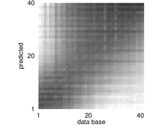
FIG. 2.: Mutual predictions between sections of length 1000 for the baker map time series used in Fig. 1.

As a realistic example, we study a recording of the breath rate of a human patient during almost a whole night (about 5 h), measured twice a second. The data is part of data set B from the Santa Fe Institute time series contest held in 1992. It is described in Ref. [11]. Obviously, conditions cannot be assumed to be constant during a night’s sleep. Changes of the calibration and the instantaneous variance, as well as the linear autocorrelations are easy to detect by standard methods. In order to emphasize that the algorithm is sensitive to changes in the nonlinear structure, we subtract from the data the running mean and divide it by the running root mean squared amplitude. Further, all prediction errors are normalized to the error of the best linear AR(1) model.

FIG. 3.: Prediction error $\gamma_{ii}$ for segments of a long, nonstationary recording of the breath rate of a human.[11] The set was split into 40 segments of 850 points (425 secs.) each. Errors are normalized to the error of the best AR(1) model. Considerable fluctuations are present but there is no indication of a qualitative difference between the first and the second half of the recording.

In order to detect nontrivial changes, we split the recording into 40 nonoverlapping segments $S_{i}$ of 850 points (425 sec.) each. Cross–predictions are performed using $m=2$, and $\epsilon$ is chosen to be $0.25$ (at unit rms amplitude). In Fig. 3 we show the (auto–) prediction error $\gamma_{ii}$ as a function of segment number. There are some fluctuations, most prominent are the lower errors for segments 15–18. The cross–prediction error is shown in Fig. 4 as grey shades. Black means $\gamma\leq 0.9$, white $\gamma>1.3$, linear grey shades are used in between. Except from the lower errors for $i=j$ (see note [9]), we see that there is a transition around one third of the recording: segments up to about 15 are less useful for predictions of segments after about 20 and vice versa. That segments 15–18 are different was aparent from Fig. 3 already. For this data set, most nonlinear tests are able to detect that nonstationarity is present. The main advantage of the present method is that it provides more detailed, time resolved information than just a statement that nonstationarity has been found.

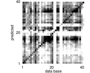
FIG. 4.: Cross–prediction errors for segments of a recording of the breath rate of a human. The figure shows that there is a qualitative change in the dynamics around segment 15.

The algorithm as described here contains a few parameters which have to be chosen appropriately for each data set. The embedding dimension $m$ and neighborhood size $\epsilon$ should yield good overall predictions. The segment size is determined by the tradeoff between statistical stability of $\gamma_{ij}$ for long segments and finer time resolution for short segments. A slight advantage may be gained by the use of overlapping segments. Other relative statistics than cross–predictions may be used and the table of the $\gamma_{ij}$ may be interpreted by other means than grey scale plotting. In particular, ongoing research is devoted to the evaluation of $\gamma_{ij}$ in terms of cluster analysis.

In a nonlinear setting, for instance if it is planned to apply algorithms from the theory of deterministic chaos to a time series, weak stationarity (constant second moments) is certainly not enough. Let us further remark that the widespread notion that the system which produces the time series must remain unchanged during the time of measurement is neither a necessary nor a sufficient condition for stationarity. The reason is that there is no a posteriori distinction between a system parameter (to remain constant) and a variable (which may evolve in time). Thus a system with a rapidly fluctuating parameter may yield a stationary time series because these fluctuations can be averaged over, while a system with constant parameters can produce signals which for all practical work must be considered nonstationary. An example for the latter case is given by intermittency where the time evolution of some variables may become arbitrarily slow. For processes, stationarity can be defined by requiring that the joint probability distribution remains constant. Given a finite time series, this probability distribution can only be estimated up to statistical fluctuations. It is problematic to define stationarity on the base of such an estimate. In this paper we have taken a rather pragmatic point of view and call a signal stationary if anything which changes in time (no matter if we call it a variable or a parameter) does so on a time scale such that the changes average out over times much smaller than the duration of the measurement.

We were able to detect changes in the dynamics of a system even if scalar statistics do not change significantly. The proposed method is meant to augment known tests for stationarity, in particular since it includes the possibility to find interrelations and similarities between different parts of a time series.

We thank Holger Kantz and Peter Grassberger for useful comments. This work was supported by the SFB 237 of the Deutsche Forschungsgemeinschaft.

REFERENCES

- [1] M. B. Priestley, “Non–linear and Non–stationary Time Series Analysis”, Academic Press, London (1988).
- [2] H. Isliker and J. Kurths, Int. J. Bifurcation and Chaos 3 1573 (1993).
- [3] A. Provenzale, L. A. Smith, R. Vio, and G. Murante, Physica D 58 31 (1992).
- [4] J. P. Eckmann, S. Oliffson Kamphorst, and D. Ruelle, Europhys. Lett. 4 973 (1987).
- [5] M. B. Kennel, Statistical test for dynamical nonstationarity in observed time-series data, preprint (1995)
- [6] R. Manuca and R. Savit, Stationarity and nonstationarity in time series analysis, to appear in Physica D (1996); G. Sugihara, B. Grenfell, and R. M. May, Phil. Trans. R. Soc. Lond. B 330 235 (1990); L. A. Smith, K. Godfrey, P. Fox, and K. Warwick, in Control 91, Vol. 1, 1062. IEE Conference Publication 332 (1991).
- [7] H. Kantz, Phys. Rev. E 49 5091 (1994).
- [8] L. M. Pecora, T. L. Carroll, and J. F. Heagy, Phys. Rev. E 52 3420 (1995).
- [9] Since consecutive individual prediction errors are not independent, temporal neighbors of closer than a typical correlation time must be excluded in order to obtain an out–of–sample error.
- [10] H. G. Schuster, “Deterministic Chaos: An Introduction”, Physik Verlag, Weinheim (1988).
- [11] D. R. Rigney, A. L. Goldberger, W. Ocasio, Y. Ichimaru, G. B. Moody, and R. Mark, in A. S. Weigend and N. A. Gershenfeld, editors, “Time Series Prediction: Forecasting the Future and Understanding the Past”, Santa Fe Institute Studies in the Science of Complexity, Proc. Vol. XV, Addison-Wesley (1993).