Geometrical properties of Maslov indices in periodic-orbit theory

Abstract

Maslov indices in periodic-orbit theory are investigated using phase space path integral. Based on the observation that the Maslov index is the multi-valued function of the monodromy matrix, we introduce a generalized monodromy matrix in the universal covering space of the symplectic group and show that this index is uniquely determined in this space. The stability of the orbit is shown to determine the parity of the index, and a formula for the index of the n-repetition of the orbit is derived.

PACS numbers: 05.45.Mt, 02.40.Ma

Over the past few decades a large number of studies have been made on periodic-orbit theory [1]. However, the Maslov index, which is an additional phase factor appearing in periodic orbit theory, doesn’t seem to be thoroughly understood. For hyperbolic orbits, Robbins [2] showed that these indices are the winding numbers which are defined by the invariant Lagrangian manifolds around these orbits. Moreover, it was conjectured that the same argument could be extended to elliptic orbits and more general orbits which have mixed stability. However, this is not the case since general orbits don’t necessarily have such invariant manifolds around them. Furthermore, Brack et al. [3] investigated periodic orbits in anisotropic harmonic oscillator (these orbits are elliptic), and showed the Maslov index of the n-repetition of the orbit $\mu_{n}$ is not equal to $n\mu_{1}$. This result contradicts Robbins’s conjecture, which leads to $\mu_{n}=n\mu_{1}$.

In this letter, we propose a new approach to the problem which can be applied to all periodic orbits, irrespective of the type of the stability. Our method is based on phase space path integral of the partition function. The advantage of using phase space path integral is that it respects symmetries of the system: time translation symmetry and canonical invariance. In addition to global canonical transformations, our method allows us to use local canonical transformations which act differently at each point of the orbit. They are regarded as gauge transformations with gauge group ${\rm Sp}(2n,R)$, and the topological nature of this gauge group plays essential role in our theory. Derivation of semiclassical trace formula using phase space path integral was given by Sakita et al.[7], and similar analysis was made by Kuratsuji [8] for coherent state path integral, but Maslov indices are neglected in these works. Maslov indices of semicalassical propagator (but not the periodic orbit) was investigated by Levit et al. [5, 6] using phase space path integral, and they showed that this index is given by the excess of the negative eigenvalues of second variation of action around the orbit. We treat Maslov indices of periodic orbits in the same way as theirs. There are two types of Maslov indices of periodic orbits: indices for the partition function (time region), and that for the density of states (energy region). We calculate Maslov indices for the partition function first. Then it is easy to calculate Maslov indices for the density of states by taking into account the extra phase contributions that arises in performing the Fourier-Laplace transform by the stationary phase approximation.

The main idea of this paper is that the linearized symplectic flow around the orbit directly determines the Maslov index. Therefore we don’t use Lagrangian manifolds in this paper. The linearized symplectic flow is represented by $V(t)$ (a symplectic matrix with one parameter $t$), and $V(t)$ is considered to be a curve on the group manifold of ${\rm Sp(2n,R)}$. We can see various properties of Maslov indices by continuous deformation of this curve.

Our final results can be summarized in the following formula eq.(1) and eq.(2). The Maslov index of the orbit is

$$\mu=p+q+2k,$$ (1)

where $p$ is the numbers of elliptic pairs of eigenvalues, $q$ is the number of inverse hyperbolic pairs of eigenvalues, and $k$ is the winding number which will be defined later on. We can see that parity of the index is determined by $p$ and $q$ from this formula. The Maslov index of the n-repetition of this orbit is

$$\mu_{n}=\sum_{i=1}^{p}\left(1+2\left[\frac{n\alpha_{i}}{2\pi}\right]\right)+nq+2nk,$$ (2)

where $\alpha_{i}$ is the stability angle of the i-th elliptic eigenvalues. Note that $\mu_{n}$ is not equal to $n\mu_{1}$ if the orbit have elliptic eigenvalues.

Let us start with the following identity for the density of states;

$$\rho(E)=-\frac{1}{\pi}{\rm Im}\;g(E+i\epsilon),$$ (3)

$$g(E)=\mbox{${\rm Tr}$}\frac{1}{E-\hat{H}}.$$ (4)

$g(E)$ is obtained by Fourier-Laplace transform of the partition function:

$$g(E)=\frac{1}{i\hbar}\int_{0}^{\infty}dTe^{iET/\hbar}Z(T).$$ (5)

We use the phase space path integral of the partition function:

$$Z(T)={\rm Tr}\exp\left[-\frac{i}{\hbar}\hat{H}T\right]=\int{\cal D}\mbox{\boldmath$p$}{\cal D}\mbox{\boldmath$q$}\exp\left[\frac{i}{\hbar}\oint(\mbox{\boldmath$p$}d\mbox{\boldmath$q$}-Hdt)\right].$$ (6)

Strictly speaking, we should write (6) in a discrete form to obtain well-defined continuum limit. However, to make the discussion simple and show our essential idea, we use continuum notation throughout this paper. The detailed analysis of (6), including subtle problems concerning operator ordering and changing variables, will be reported in the forthcoming paper. [13].

Let us evaluate (6) by the stationary phase approximation. The stationary phase condition reads

$$\delta\oint(\mbox{\boldmath$p$}d\mbox{\boldmath$q$}-Hdt)=0,$$ (7)

which leads to the Hamilton equations of motion. It follows from the periodic boundary condition of the path integral that the solutions of (7) are periodic orbits. Thus the semi-classical approximation $Z_{sc}(T)$ to $Z(T)$ is given by a sum over the periodic orbits.

$$Z_{sc}(T)=\sum_{p.o.}K\exp\left[\frac{i}{\hbar}R\right].$$ (8)

Here $R=\oint(\mbox{\boldmath$p$}d\mbox{\boldmath$q$}-Hdt)$ is the classical action of the periodic-orbit, and $K$ is the contribution of the quadratic fluctuation around the orbit,

$$K=\int{\cal D}\mbox{\boldmath$x$}\exp\left[i\delta^{2}R[\mbox{\boldmath$x$}(t)]\right],$$ (9)

$$\mbox{\boldmath$x$}(t)=\frac{1}{\sqrt{\hbar}}(\delta p_{1},\delta q_{1},\delta p_{2},.....,\delta q_{n})$$ (10)

The explicit form of the second variation $\delta^{2}R$ is

$$\delta^{2}R[\mbox{\boldmath$x$}(t)]=\frac{1}{2}\int_{0}^{T}dt\;\mbox{\boldmath$x$}^{T}(t)\left(-J\frac{d}{dt}-H^{{}^{\prime\prime}}(\mbox{\boldmath$p$}(t),\mbox{\boldmath$q$}(t))\right)\mbox{\boldmath$x$}(t),$$ (11)

where $J$ is a matrix of the form:

$$J=\left(\begin{array}[]{ccccc}j&&&&\\ &j&&&\\ &&.&&\\ &&&.&\\ &&&&j\end{array}\right),$$ (12)

and $j$ is a $2\times 2$ matrix:

$$j=\left(\begin{array}[]{cc}0&-1\\ 1&0\end{array}\right).$$ (13)

We rewrite (11) as

$$\delta^{2}R=-\frac{1}{2}\int_{0}^{1}dt^{{}^{\prime}}\mbox{\boldmath$x$}^{T}(t^{{}^{\prime}})\mbox{$D\hskip-6.49994pt/\;$}(t^{{}^{\prime}})\mbox{\boldmath$x$}(t^{{}^{\prime}}),$$ (14)

where $t^{{}^{\prime}}=t/T$, and $D\hskip-6.49994pt/\;$ is defined as

$$\mbox{$D\hskip-6.49994pt/\;$}(t)=JD=J\left(\frac{d}{dt}-A(t)\right),$$ (15)

$$A(t)=TJ\;H^{{}^{\prime\prime}}(\mbox{\boldmath$p$}(t/T),\mbox{\boldmath$q$}(t/T)).$$ (16)

$A$ is the connection for the displacement vector $x$, and $D=d/dt-A$ is the covariant derivative. The parallel transport of $x$ is defined by the equation $D\mbox{\boldmath$x$}=0$ (Fig.1), which is the Hamiltonian equation of motion for $x$:

$$\frac{d}{dt}\mbox{\boldmath$x$}=JH^{{}^{\prime\prime}}\left(\mbox{\boldmath$p$}(t),\mbox{\boldmath$q$}(t)\right)\mbox{\boldmath$x$}.$$ (17)

Hereafter we slightly generalize the problem, and $A$ is considered to be a generator of symplectic group which satisfies $A^{T}J+JA=0$. Then $A$ is written as

$$A(t)=JH(t),$$ (18)

where $H$ is a symmetric matrix of even demension. (16) is the special case of (18). We deal with the quadratic path integral of the following form instead of (9):

$$K=\int{\cal D}\mbox{\boldmath$x$}\exp\left[-\frac{i}{2}\mbox{\boldmath$x$}^{T}\mbox{$D\hskip-6.49994pt/\;$}\mbox{\boldmath$x$}\right]=\frac{1}{\sqrt{\mbox{${\rm Det}\>$}i\mbox{$D\hskip-6.49994pt/\;$}}}$$ (19)

Here $\mbox{$D\hskip-6.49994pt/\;$}=J(d/dt-A)$, and $A$ is defined in (18). The phase of (19) defines the Maslov index:

$$\frac{1}{\sqrt{\mbox{${\rm Det}\>$}i\mbox{$D\hskip-6.49994pt/\;$}}}=\frac{e^{-i\pi\mu/2}}{\sqrt{|\mbox{${\rm Det}\>$}\mbox{$D\hskip-6.49994pt/\;$}|}}$$ (20)

$$\mu=\frac{\mu_{+}-\mu_{-}}{2}.$$ (21)

Here $\mu_{+}(\mu_{-})$ denote the number of the positive (negative) eigenvalues of $D\hskip-6.49994pt/\;$. In the continuum limit, both $\mu_{+}$ and $\mu_{-}$ become infinity, and the formula (21) cannot directly define the Maslov index. However, we can evaluate the relative change of the index by deforming the operator $D\hskip-6.49994pt/\;$ continuously and analyzing the points where the sign of the eigenvalue changes. (This is similar to the discussion given in [5, 6] for the semi-classical propagator.)

In the following, we calculate $|\mbox{${\rm Det}\>$}\mbox{$D\hskip-6.49994pt/\;$}|$ and $\mu$ in (20). The procedure consists of three steps.

1. Diagonalization of $D$ and calculation of $|\mbox{${\rm Det}\>$}\mbox{$D\hskip-6.49994pt/\;$}|=|\mbox{${\rm Det}\>$}D|$.

2. Diagonalization of $D\hskip-6.49994pt/\;$ using the basis given in the first step.

3. Calculation of $\mu$ by continuous deformations of $D\hskip-6.49994pt/\;$.

The first step is essentially the same as the discussions given in [7] and [8]. The second and the third steps are first given in this paper.

The first step is the calculation of $|\mbox{${\rm Det}\>$}\mbox{$D\hskip-6.49994pt/\;$}|$. For this purpose, we first diagonalize the covariant derivative $D$:

$$D\mbox{\boldmath$x$}=\left(\frac{d}{dt}-A\right)\mbox{\boldmath$x$}=\epsilon\mbox{\boldmath$x$}.$$ (22)

This equation is easy to solve because the time derivative has diagonal form. We introduce a symplectic matrix $V(t)$ which stands for the flow around the orbit:

$$DV(t)=0.$$ (23)

If we fix $V(0)=1$, $D$ and $V$ has one to one correspondence, and $V(1)\;(=M)$ is the monodromy matrix of the orbit. Let $\mbox{\boldmath$\xi$}_{\zeta}$ be the eigenvector of M, and $\zeta$ be the stability angle of the orbit,

$$M\mbox{\boldmath$\xi$}_{\zeta}=e^{-i\zeta}\mbox{\boldmath$\xi$}_{\zeta}.$$ (24)

Then the solutions of (22) are written as follows:

$$\mbox{\boldmath$x$}_{\zeta,n}(t)=\exp(\epsilon_{\zeta,n}t)V(t)\mbox{\boldmath$\xi$}_{\zeta},$$ (25)

$$D\mbox{\boldmath$x$}_{\zeta,n}=\epsilon_{\zeta,n}\mbox{\boldmath$x$}_{\zeta,n},$$ (26)

$$\epsilon_{\zeta,n}=(\zeta+2n\pi)i.$$ (27)

If $e^{-i\zeta}$ is the eigenvalue of $M$, $e^{i\zeta}$ also becomes the eigenvalue of $M$ [4], and the absolute value of the functional determinant of $D\hskip-6.49994pt/\;$ can be evaluated as a product of eigenvalues (27):

$$|\mbox{${\rm Det}\>$}\mbox{$D\hskip-6.49994pt/\;$}|=|\mbox{${\rm Det}\>$}D| = \prod_{n,l}\left|(2\pi n)^{2}-\zeta_{l}^{2}\right|,$$ (28)

$$\sim \left|\prod_{l}\zeta_{l}^{2}\prod_{n=1}^{\infty}\left(1-\left(\frac{\zeta_{l}}{2n\pi}\right)^{2}\right)\right|.$$ (29)

Here we replace the divergent constant $\prod_{n=1}^{\infty}2\pi n$ by 1. In discrete formalism, this term corresponds to

$$\frac{1}{N}\prod_{n=1}^{N-1}2\sin\frac{\pi n}{N}=1.$$ (30)

For $n\ll N$, $\prod_{n}2\sin\pi n/N\sim\prod_{n}2\pi n/N$, therefore (30) is considered to be a normalized value of $\prod_{n=1}^{\infty}2\pi n$. Details of this renormalization procedure will be given in [13].

The result is

$$|\mbox{${\rm Det}\>$}\mbox{$D\hskip-6.49994pt/\;$}| = \left|\prod_{l}\left(2\sin\frac{\zeta_{l}}{2}\right)^{2}\right|,$$ (31)

$$= |\det(M-I)|.$$ (32)

Here we used the formula

$$\prod_{n=1}^{\infty}\left(1-\frac{x^{2}}{n^{2}}\right)=\frac{\sin\pi x}{\pi x}.$$ (33)

The second step is the diagonalization of $D\hskip-6.49994pt/\;$. If we represent $D\hskip-6.49994pt/\;$ using the basis (25), it is easy to see that $D\hskip-6.49994pt/\;$ is the block diagonal matrix. We can obtain diagonal representation of $D\hskip-6.49994pt/\;$ by diagonalizing this block diagonal matrix again.

First we assume that $M$ has no degenerate eigenvalue. If $\zeta$ is a stability angle of the orbit, $-\zeta$ and $\zeta^{*}$ are also stability angles of the orbit because $M$ is the symplectic matrix [4]. Therefore eigenvalues of $M$ can be classified into four types, and $M$ can be transformed into a block diagonal matrix by a symplectic transformation.

$$M=\left(\begin{array}[]{ccccc}m_{1}&&&&\\ &m_{2}&&&\\ &&.&&\\ &&&.&\\ &&&&m_{k}\\ \end{array}\right)$$ (34)

1. elliptic: $\zeta=\pm\alpha$

   $$m=\left(\begin{array}[]{cc}\cos\alpha&-\sin\alpha\\ \sin\alpha&\cos\alpha\end{array}\right)$$ (35)

2. hyperbolic: $\zeta=\pm i\beta$

   $$m=\left(\begin{array}[]{cc}e^{\beta}&0\\ 0&e^{-\beta}\end{array}\right)$$ (36)

3. inverse hyperbolic: $\zeta=\pm i(\beta+\pi)$

   $$m=\left(\begin{array}[]{cc}-e^{\beta}&0\\ 0&-e^{-\beta}\end{array}\right)$$ (37)

4. loxodromic: $\zeta=\pm\alpha\pm i\beta$

   $$m=\left(\begin{array}[]{cccc}e^{\beta}\cos\alpha&0&-e^{\beta}\sin\alpha&0\\ 0&e^{-\beta}\cos\alpha&0&-e^{-\beta}\sin\alpha\\ e^{\beta}\sin\alpha&0&e^{\beta}\cos\alpha&0\\ 0&e^{-\beta}\sin\alpha&0&e^{-\beta}\cos\alpha\end{array}\right)$$ (38)

The matrix elements between $\mbox{\boldmath$x$}_{\zeta,n}$ and $\mbox{\boldmath$x$}_{\zeta^{{}^{\prime}},n^{{}^{\prime}}}$ are non-zero only if $\zeta$ and $\zeta^{{}^{\prime}}$ belong to the same block. Therefore it is enough to diagonalize each block separately to diagonalize $D\hskip-6.49994pt/\;$.

For example, eigenvalues and eigenvectors which belong to a hyperbolic block are

$$M\mbox{\boldmath$x$}_{\pm}=e^{\pm\beta}\mbox{\boldmath$x$}_{\pm}.$$ (39)

Here, the normalization condition is taken as

$$[\mbox{\boldmath$x$}_{+},\mbox{\boldmath$x$}_{-}]=1,$$ (40)

and eigenvalues and eigenvectors of $D$ are

$$D\mbox{\boldmath$x$}_{\pm,n}(t)=\epsilon_{\pm,n}\mbox{\boldmath$x$}_{\pm,n}(t),$$ (41)

$$\mbox{\boldmath$x$}_{\pm,n}(t)=\exp(\epsilon_{\pm,n})V(t)\mbox{\boldmath$x$}_{\pm}(t),$$ (42)

$$\epsilon_{\pm,n}=\mp\beta+2n\pi i.$$ (43)

We define real vectors $\mbox{\boldmath$x$}_{c,\pm,n},\mbox{\boldmath$x$}_{s,\pm,n}$ as

$$\mbox{\boldmath$x$}_{c,\pm,n} = \frac{1}{\sqrt{2}}(\mbox{\boldmath$x$}_{\pm,n}+\mbox{\boldmath$x$}_{\pm,-n}),$$ (44)

$$\mbox{\boldmath$x$}_{s,\pm,n} = \frac{1}{\sqrt{2}i}(\mbox{\boldmath$x$}_{\pm,n}-\mbox{\boldmath$x$}_{\pm,-n})\;\;\;(n=1,2,...).$$ (45)

Since $\mbox{\boldmath$x$}_{\pm,0}$ are real vectors, we don’t have to re-define them. Matrix elements which have non-zero values are

$$\int_{0}^{1}\!dt\;\mbox{\boldmath$x$}_{c,+,n}^{T}\mbox{$D\hskip-6.49994pt/\;$}\mbox{\boldmath$x$}_{c,-,n} = -\beta,$$ (46)

$$\int_{0}^{1}\!dt\;\mbox{\boldmath$x$}_{s,+,n}^{T}\mbox{$D\hskip-6.49994pt/\;$}\mbox{\boldmath$x$}_{c,-,n} = -2n\pi,$$ (47)

$$\int_{0}^{1}\!dt\;\mbox{\boldmath$x$}_{c,+,n}^{T}\mbox{$D\hskip-6.49994pt/\;$}\mbox{\boldmath$x$}_{s,-,n} = 2n\pi,$$ (48)

$$\int_{0}^{1}\!dt\;\mbox{\boldmath$x$}_{s,+,n}^{T}\mbox{$D\hskip-6.49994pt/\;$}\mbox{\boldmath$x$}_{c,-,n} = -\beta,$$ (49)

$$\int_{0}^{1}\!dt\;\mbox{\boldmath$x$}_{+,0}^{T}\mbox{$D\hskip-6.49994pt/\;$}\mbox{\boldmath$x$}_{-,0} = -\beta.$$ (50)

Therefore $D\hskip-6.49994pt/\;$ is represented by the matrix $d_{n}$ in the space spanned by $\mbox{\boldmath$x$}_{c,\pm,n},\mbox{\boldmath$x$}_{s,\pm,n}$:

$$d_{n}=\left(\begin{array}[]{cccc}0&0&-\beta&2n\pi\\ 0&0&-2n\pi&-\beta\\ -\beta&-2n\pi&0&0\\ 2n\pi&-\beta&0&0\end{array}\right)\;\;\;(n\geq 1).$$ (51)

In the case of $n=0$,

$$d_{0}=\left(\begin{array}[]{cc}0&-\beta\\ -\beta&0\\ \end{array}\right).$$ (52)

The solutions of the eigenvalue equation $\det(d_{n}-\lambda I)=0$ are

$$\lambda = \pm\sqrt{\beta^{2}+(2n\pi)^{2}}\;\;\;\;(n\geq 1),$$ (53)

$$\lambda = \pm\beta\;\;\;\;(n=0).$$ (54)

The solutions for $n\geq 1$ are doubly degenarate. Thus we obtain diagonal representation of $D\hskip-6.49994pt/\;$ for hyperbolic blocks.

Other blocks can be treated in the same way. First, we define real basis from the real parts and the imaginary parts of the basis (25), and represent $D\hskip-6.49994pt/\;$ using this basis. Then $D\hskip-6.49994pt/\;$ become a block diagonal matrix and each block is $4\times 4$ at most. Second, we diagonalize these blocks, then we obtain diagonal representation of $D\hskip-6.49994pt/\;$.

Diagonal elements of an elliptic block are

$$\alpha+2n\pi\;\;\;(n=0,\pm 1,\pm 2,...).$$ (55)

For a inverse hyperbolic block,

$$\pm\sqrt{\beta^{2}+(2n+1)^{2}}\;\;\;(n=0,1,2,...).$$ (56)

For a loxodromic block,

$$\pm\sqrt{\beta^{2}+(\alpha+2n\pi)^{2}}\;\;\;(n=0,\pm 1,\pm 2...).$$ (57)

All diagonal elements are doubly degenerate. These results are summarized in Table 1.

Till now, we have assumed that the monodromy matrix $M$ has no degenerate eigenvalue. If $M$ has degenerate eigenvalues, we have to deal with these cases separately. We will not go into the details of these exceptional cases, but the case in which $M$ has eigenvalue 1 is very important. In this case, the stability angle of the eigenvalue is 0, which means that $D\hskip-6.49994pt/\;$ USA a zero-mode and the orbit is not isolated. Therefore we have to calculate the functional determinant of $D\hskip-6.49994pt/\;$ in the space where the zero-mode is removed (we denote this as $\mbox{${\rm Det}\>$}^{{}^{\prime}}\mbox{$D\hskip-6.49994pt/\;$}$), and integrate with respect to the zero-mode separately.

We deal with the simplest case in which the eigenvalue 1 is doubly degenerate.(This type is called parabolic.) We can choose the basis $\mbox{\boldmath$x$}_{\alpha}\;(\alpha=1,2)$ as

$$M\mbox{\boldmath$x$}_{1} = \mbox{\boldmath$x$}_{1},$$ (58)

$$M\mbox{\boldmath$x$}_{2} = \mbox{\boldmath$x$}_{2}+\gamma\mbox{\boldmath$x$}_{1},$$ (59)

$$[\mbox{\boldmath$x$}_{1},\mbox{\boldmath$x$}_{2}]=1.$$ (60)

In this case, the basis (25) are not complete set. Therefore we define new basis as

$$\mbox{\boldmath$x$}_{\alpha,n}(t) = V(t)\exp\left[t(2n\pi iI-B)\right]\mbox{\boldmath$x$}_{\alpha}\;\;\;(\alpha=1,2).$$ (61)

Here, $I$ is the unit matrix, and $B$ is defined as

$$B\mbox{\boldmath$x$}_{1} = 0,$$ (62)

$$B\mbox{\boldmath$x$}_{2} = \gamma x_{1}.$$ (63)

Note that $B$ is the generator of $M$($e^{B}\mbox{\boldmath$x$}_{\alpha}=M\mbox{\boldmath$x$}_{\alpha}$). $D$ acts on these basis as

$$D\mbox{\boldmath$x$}_{1,n} = 2n\pi i\mbox{\boldmath$x$}_{1,n},$$ (64)

$$D\mbox{\boldmath$x$}_{2,n} = 2n\pi i\mbox{\boldmath$x$}_{2,n}-\gamma\mbox{\boldmath$x$}_{1,n}.$$ (65)

We define real basis as in (45), then $D\hskip-6.49994pt/\;$ is represented in this space as

$$d_{n}=\left(\begin{array}[]{cccc}0&0&0&2n\pi\\ 0&0&-2n\pi&0\\ 0&-2n\pi&\gamma&0\\ 2n\pi&0&0&\gamma\\ \end{array}\right)\;\;\;(n\geq 1),$$ (66)

$$d_{0}=\left(\begin{array}[]{cc}0&0\\ 0&\gamma\end{array}\right).$$ (67)

The functional determinant of this part (except zero-mode) is

$$\mbox{${\rm Det}\>$}^{{}^{\prime}}\mbox{$D\hskip-6.49994pt/\;$} = \gamma\prod_{n=1}^{\infty}(2\pi n)^{4},$$ (68)

$$\sim \gamma.$$ (69)

The integration of the zero-mode must be done separately.

If $D\hskip-6.49994pt/\;$ is derived from the stationary phase approximation of the time-independent Hamiltonian system, it has at least one zero-mode corresponding to time-translation symmetry. In this case $\gamma=-dT/dE$ [10], and the result of the integration of the zero-mode is proportional to the period $T$:

$$K=\frac{T}{\sqrt{2\pi\hbar\frac{1}{i}\frac{dT}{dE}}\sqrt{|\det(M^{{}^{\prime}}-I)|}}.$$ (70)

Here $M^{{}^{\prime}}$ denote the monodromy matrix whose parabolic part is removed. The factor $\sqrt{2\pi\hbar\frac{1}{i}\frac{dT}{dE}}$ is canceled by the Fourier transformation (5), then we obtain the well-known amplitude factor of the Gutzwiller trace formula:

$$\frac{T}{i\hbar\sqrt{|\det(M^{{}^{\prime}}-I)|}}.$$ (71)

Details of the integration of the zero-mode will be discussed in [13].

The third step is the calculation of the Maslov index $\mu$. If $A=0$, the Maslov index is considered to be 0, and we can see relative changes of the Maslov index by continuously deforming the operator $D\hskip-6.49994pt/\;$. Thus we can calculate the Maslov index. The point is that the deformation of $D\hskip-6.49994pt/\;$ corresponds to that of $V(t)$. $V(t)$ is a curve on the symplectic group, therefore deformation of $D\hskip-6.49994pt/\;$ means deformation of the curve on the symplectic group. If we continuously deform the curve without changing the initial point (origin) and the end point (monodromy matrix), the Maslov index of the curve doesn’t change because the diagonal elements are determined only by the monodromy matrix and don’t change during the deformation. Therefore we regard such curves are equivalent (Fig.2). (We refer this equivalence relation as $\sim$.) This means that we can regard two operator $\mbox{$D\hskip-6.49994pt/\;$}(A)$ and $\mbox{$D\hskip-6.49994pt/\;$}(A^{{}^{\prime}})$ equivalent if $A$ and $A^{{}^{\prime}}$ are connected by a continuous gauge transformation.

However, if two curves which have the same terminal points can’t be shrunk to a point continuously, two curves doesn’t necessarily have the same Maslov index. Such cases actually happen, because symplectic groups have non-trivial topology and the fundamental group of them are [11]

$$\pi_{1}({\rm Sp}(2n,R))=Z.$$ (72)

In other words, the Maslov index (and the path integral (19)) is the multi-valued function of the monodromy matrix. The Maslov index is completely determined by the curve on the symplectic group starting from the origin (we refer this set of curves as F), then the Maslov index is uniquely determined on the quotient space $F/\sim$, and this is exactly the definition of the universal covering space;

$$F/\sim\;\;=\tilde{{\rm Sp}}(2n,R).$$ (73)

Therefore the Maslov index is regarded as the function on $\tilde{{\rm Sp}}(2n,R)$, instead of ${\rm Sp}(2n,R)$. This is similar to the construction of Riemann surface of the complex multi-valued function, for example, $\log z$.

A point on $\tilde{{\rm Sp}}(2n,R)$ is specified by two quantities: a symplectic matrix and a winding number. First we investigate the change of the Maslov index which comes from the winding number. For example, if we continuously change $\alpha$ to $\alpha+2\pi$ in elliptic case, the Maslov index changes by 2. Therefore in this case the change of the winding number by 1 corresponds to the change of the Maslov index by 2 (Fig.3). This rule can be applied to all cases, which can be proven as follows.

Let $A1$ and $A2$ be curves on the symplectic group. We assume that both have the same terminal points and difference of the winding number between $A1$ and $A2$ is 1. Then deform $A1$ continuously to $A2$ through the other curves $B1,B2$ (Fig.4). The difference of the Maslov index between $A1$ and $A2$ is the same as that of $B1$ and $B2$, because the change of the Maslov index during the deformation $A1\rightarrow B1$ is canceled by that of $B2\rightarrow A2$ if the end-point go through the same path during the two processes. Therefore the rule that holds for some cases holds for all cases, and the change of the winding number by 1 corresponds to the change of the Maslov index by 2, regardless of the stability. This means that $(\mbox{${\rm Det}\>$}i\mbox{$D\hskip-6.49994pt/\;$})^{1/2}$ changes sign by the gauge transformation $U$ that changes the winding number by odd number:

$$\{\mbox{${\rm Det}\>$}i\mbox{$D\hskip-6.49994pt/\;$}(A^{U})\}^{1/2}=-\{\mbox{${\rm Det}\>$}i\mbox{$D\hskip-6.49994pt/\;$}(A)\}^{1/2}$$ (74)

where $A^{U}$ is defined as

$$A^{U}=-U^{-1}\frac{dU}{dt}+U^{-1}AU.$$ (75)

A similar result is known in anomaly of SU(2) gauge theory coupled to Weyl fermions [12].

Now we know the contribution from the winding number to the Maslov index, the next question is the contribution from the monodromy matrix. Since the winding number changes the Maslov index by a multiple of 2, the monodromy matrix determines whether the index is even or odd. The Maslov index changes at the point where $D\hskip-6.49994pt/\;$ has zero eigenvalues, and this means the monodromy matrix has the eigenvalue 1. (This is the condition for bifurcation.) Therefore the Maslov index changes when end-point of $V$ crosses the region defined by $\det(M-I)=0$ (Fig.5).

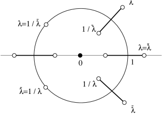
Figure 6: eigenvalues of a sympectic matrix in the complex plane.

In Fig.6, we show eigenvalues of the monodromy matrix in the complex plane. The stability changes when eigenvalues collide, and collisions are classified as follows:

1. elliptic $\leftrightarrow$ hyperbolic
   two eigenvalues collide at 1

2. elliptic $\leftrightarrow$ inverse hyperbolic
   two eigenvalues collide at -1

3. elliptic($\times 2$) $\leftrightarrow$ loxodromic
   eigenvalues collide simultaneously at conjugate points of the unite circle

The Maslov index changes when eigenvalues collide at the point 1, and we can see from table1 that the parity of the Maslov index changes when and only when the stability changes elliptic $\leftrightarrow$ hyperbolic.

A given curve $C$ on the symplectic group can be deformed into a normal form $U_{k}C^{{}^{\prime}}$ using continuous deformation (Fig.8). $U_{k}$ is the closed curve which have the winding number $k$, and $C^{{}^{\prime}}$ is defined not to cross bifurcation regions. Since the monodromy matrix can be decomposed into some blocks, $C^{{}^{\prime}}$ can also be decomposed into these normal forms:

• elliptic

  $$\left(\begin{array}[]{cc}\cos\alpha t&-\sin\alpha t\\ \sin\alpha t&\cos\alpha t\end{array}\right)$$ (77)

• hyperbolic

  $$\left(\begin{array}[]{cc}e^{\beta t}&0\\ 0&e^{-\beta t}\end{array}\right)\\$$ (78)

• inverse hyperbolic

  $$\left(\begin{array}[]{cc}\cos 2\pi t&-\sin 2\pi t\\ \sin 2\pi t&\cos 2\pi t\end{array}\right)\;\;\;(0\leq t\leq\frac{1}{2})$$ (79)

  $$\left(\begin{array}[]{cc}-e^{2\beta(t-1/2)}&0\\ 0&-e^{-2\beta(t-1/2)}\end{array}\right)\;\;\;(\frac{1}{2}\leq t\leq 1)\\$$ (80)

• loxodromic

  $$\left(\begin{array}[]{cccc}e^{\beta t}\cos\alpha t&0&-e^{\beta t}\sin\alpha t&0\\ 0&e^{-\beta t}\cos\alpha t&0&-e^{-\beta t}\sin\alpha t\\ e^{\beta t}\sin\alpha t&0&e^{\beta t}\cos\alpha t&0\\ 0&e^{-\beta t}\sin\alpha t&0&e^{-\beta t}\cos\alpha t\end{array}\right)\\$$ (81)

• parabolic

  $$\left(\begin{array}[]{cc}1&\gamma t\\ 0&1\end{array}\right)$$ (82)

The elliptic and the inverse hyperbolic type have the Maslov index 1,hyperbolic and loxodromic type have 0. Therefore if the monodromy matrix have p elliptic blocks and q inverse hyperbolic blocks, the Maslov index of the system is

$$\mu=p+q+2k$$ (83)

If the monodromy matrix have parabolic blocks, we must add $\sum_{i}\frac{1}{2}{\rm sgn}\gamma_{i}$ to the Maslov index. But the factor corresponding to time translation symmetry is canceled by the Fourier transformation.

We are now able to calculate n-repetition of this orbit. Since $C^{n}=U_{k}C^{{}^{\prime}}U_{k}C^{{}^{\prime}}....U_{k}C^{{}^{\prime}}$ can be deformed into $U_{kn}C^{{}^{\prime}n}$, we only have to consider n-th power of the normal forms. The elliptic type increases the winding number when $n\alpha$ goes over $2\pi$, therefore the Maslov index of this part is $1+2[n\alpha/2\pi]$. The square of the inverse hyperbolic type becomes hyperbolic type, and the Maslov index increase by 1. The cube of it is inverse hyperbolic, the Maslov index increases by 1, and so on. Therefore the Maslov index of this part is n. The hyperbolic type, the loxodromic type, and parabolic type don’t change the Maslov index when we raise them to n-th power. Thus the Maslov index of the n-repetition of the orbit is

$$\mu_{n}=\sum_{i=1}^{p}\left(1+2\left[\frac{n\alpha_{i}}{2\pi}\right]\right)+qn+2nk,$$ (84)

where $\alpha_{i}$ denotes the stability angle of i-th elliptic block. Note that $\mu_{n}\neq n\mu_{1}$ if the orbit has elliptic blocks.

In conclusion, we have derived the semi-classical trace formula using phase space path integral. The point is that quadratic path integral around the periodic orbit is determined by the symplectic flow around the orbit, and the flow is regarded as a curve on symplectic group. We directly diagonalize the quadratic path integral, and Maslov indices are defined by the signs of these diagonal elements. Since they are determined only by the monodromy matrix, two curves on symplectic group which have the same terminal points and can be shrunk to a point is considered to be equivalent. The set of curves divided by this equivalence relation become universal covering space of symplectic group, and Maslov indices are uniquely determined in this space. A point in the space is specified by a symplectic matrix and a winding number. The winding number changes the Maslov index by 2, and the stability of the orbit determines the parity of the Maslov index. We also derived the formula for the Maslov index of n-repetition of a orbit. If the monodromy matrix of the orbit have elliptic eigenvalues, $\mu_{n}$ is not generally equal to $n\mu_{1}$, as pointed out by Brack et al.[3]

The author would like to thank Professor T.Hatsuda for helpful discussions and encouragements. He would also like to thank Professor M.Sano, Dr. S.Sugimoto, Professor T.Kunihiro, Professor H.Kuratsuji, Professor A.G.Magner and the members of the Nuclear Theory Group at Kyoto University for valuable discussions.

stability	$\lambda$	diagonal elements	$|\mbox{${\rm Det}\>$}\mbox{$D\hskip-6.49994pt/\;$}|$	index
elliptic	$e^{\pm i\alpha}$	$\alpha+2n\pi$	$4\sin^{2}\alpha/2$	odd
hyperbolic	$e^{\pm\beta}$	$\pm\beta,\pm\sqrt{\beta^{2}+(2n\pi)^{2}}$	$4\sinh^{2}\beta/2$	even
inverse hyperbolic	$-e^{\pm\beta}$	$\pm\sqrt{\beta^{2}+(2n+1)^{2}\pi^{2}}$	$4\cosh^{2}\beta/2$	odd
loxodromic	$e^{\pm i\alpha\pm\beta}$	$\pm\sqrt{\beta^{2}+(\alpha+2n\pi)^{2}}$	$4(\cosh\beta-\cos\alpha)^{2}$	even

Table 1: Stability, eigenvalues of the monodromy matirx, diagonal elements of $D\hskip-6.49994pt/\;$, functional determinant $D\hskip-6.49994pt/\;$ of the part, and the parity of the Maslov index. All diagonal elements are doubly degenerate except $\pm\beta$ in hyperbolic case. $n$ runs over all integers in elliptic and loxodromic cases. In hyperbolic case, $n\geq 1$, and in inverse hyperbolic case, $n\geq 0$.

Figure 1: The space of the displacement vectors is regarded as fibre bundle, and Hamiltonian symplectic flow defines the connection. The structure group of this space is ${\rm Sp}(2n,R).$

Figure 2: Curves on the symplectic group. A and B is equivalent and others are not.

Figure 3: Flow of diagonal elements of elliptic type when $\alpha$ changes into $\alpha+2\pi$. The values of diagonal elements in left side and the right side are the same, but the Maslov indices differ by 2.

Figure 4: Changing the windng number. A1$\rightarrow$B1$\rightarrow$B2 $\rightarrow$A2

Figure 5: The Maslov index changes at the point where the end-point of the curve crosses the region defined by $\det(M-I)=0$.

Figure 7: The change of the sign of the diagonal element of $D\hskip-6.49994pt/\;$ when the stabilty changes elliptic to hyperbolic.

Figure 8: Deformation of a given curve $C$ into a normal form $U_{k}C^{{}^{\prime}}$. $U_{k}$ starts from the origin, goes around the hole k times, and returns to the same point. $C^{{}^{\prime}}$ doesn’t cross the region defined by $\det(M-I)=0$.

References

• [1] M.C.Gutzwiller,Chaos in Classical and Quantum Mechanics, (Springer Verlag,1990).
• [2] J.M.Robbins,Nonlinearity 4(1991),343.
• [3] M.Brack and S.R.Jain,Phys.Rev.A 51(1995),3462.
• [4] V.I.Arnold,Mathematical Methods of Classical Mechanics, (Springer Verlag,1978).
• [5] S.Levit and U.Smilansky,Ann.Physics 108(1977),165.
• [6] S.Levit,K.Mรถhring,U.Smilansky and T.Dreyfus, Ann.Physics 114(1978),223.
• [7] B.Sakita, K.Kikkawa, (in Japanese)
• [8] H.Kuratsuji,Phys.Lett.108A,(1985)139.
• [9] J.Williamson,Amer.J.of Math.58-1(1936),141.
• [10] S.C.Creagh and R.G.Littlejohn,Phys.Rev.A 44(1991),836.
• [11] R.G.Littlejohn,Phys.Rep.138(1986),193.
• [12] E.Witten,Phys.Lett.B 117(1982),324.
• [13] A.Sugita, in preparation.