Lyapunov exponents and Kolmogorov-Sinai entropy for a high-dimensional convex billiard

Abstract

We compute the Lyapunov exponents and the Kolmogorov-Sinai (KS) entropy for a self-bound $N$-body system that is realized as a convex billiard. This system exhibits truly high-dimensional chaos, and $2N-4$ Lyapunov exponents are found to be positive. The KS entropy increases linearly with the numbers of particles. We examine the chaos generating defocusing mechanism and investigate how high-dimensional chaos develops in this system with no dispersing elements.

I Introduction

Billiards are simple yet nontrivial examples of systems that display classically chaotic motion. Of special importance are the Sinai billiard [1] and the Bunimovich stadium [2] since they are known to be completely chaotic. Interestingly, these two systems exhibit two different mechanisms that generate chaos. While dispersion is the chaos-generating mechanism in the Sinai billiard it is defocusing that leads to chaotic dynamics in the Bunimovich stadium. Dispersing yields a permanent divergence of neighbored trajectories. Defocusing may occur upon reflection at a focusing boundary element. Provided the free path is sufficiently long nearby trajectories start to diverge after passing through the focusing point, and on average the divergence might exceed the convergence thus leading to exponential instability. Dispersing billiards are well known also in higher dimensions. Popular examples are the three-dimensional Sinai billiard and the hard sphere gas. However, it was not until recently that completely chaotic billiards were constructed in more than two spatial dimensions that rely entirely on the defocusing mechanism [3, 4]. These billiards use spherical caps as the focusing elements of the boundary. A trajectory diverges mainly in a two-dimensional plane that is defined by the points of consecutive reflections with the spherical cap, and focusing may be very weak in the transversal directions. This makes it more difficult to create truly high-dimensional chaos in focusing billiards than in dispersing ones. Sufficient conditions for the construction of high-dimensional focusing billiards were given in ref.[3], but it was found that these are not necessary ones[4].

Besides of their intrinsic interest billiards are important model systems in the field of quantum chaos [5] and statistical and fluid mechanics [6]. Questions related to chaos, ergodicity, transport and equilibration are often studied in billiard models, see e.g. refs.[7, 8]. While two-dymensional chaos is fairly well understood by now, much less is known in high-dimensional systems. Recently, a high-dimensional billiard model has been proposed in the context of nuclear physics [9] and quantum chaos [10]. Within this model a self-bound $N$-body system is realized as a convex billiard. Numerical computations yielded a positive largest Lyapunov exponent and showed that this system is predominantly chaotic. In this article we want to extend previous calculations and compute the full Lyapunov spectrum and the KS entropy for this chaotic $N$-body system. These quantities characterize the degree of hyperbolic instability in dynamical systems and may be related to transport coefficients in non-equilibrium situations [11]. Since the studied billiard is convex, defocusing is the only possible source causing this instability [12]. This makes it interesting to examine this mechanism in more detail and compare to the situation of defocusing billiards with spherical caps. The results of such an investigation are not only of theoretical interest but may also be useful for further applications. We have in mind general questions concerning chaos in self-bound many-body systems like nuclei or atomic clusters and its influence on equilibration, damping or transport processes.

This paper is organized as follows. In the next section we describe the model system and the techniques used to compute the Lyapunov exponents. The third section contains the results of our numerical computations for various system sizes $N$. In section four we investigate the defocusing mechanism in more detail. We finally give a summary.

II High-dimensional billiard and Lyapunov exponents

Let us consider a classical system of $N$ particles with Hamiltonian

$$H=\sum_{i=1}^{N}{p_{i}^{2}\over 2m}+\sum_{i<j}V(|\vec{r}_{i}-\vec{r}_{j}|),$$ (1)

where $\vec{r}_{i}$ is a two-dimensional position vector of the $i$-th particle and $\vec{p}_{i}$ is its conjugate momentum. The interaction is given by

$$V(r)=\left\{\begin{array}[]{ll}0&\mbox{for $r<a$},\\ \infty&\mbox{for $r\geq a$}.\end{array}\right.$$ (4)

Thus, the particles move freely and interact whenever the distance between a pair of particles reaches its maximum value $a$. Hamiltonian (1) defines a self-bound, interacting many-body system. Energy, total momentum and total angular momentum are conserved quantities. For large numbers of particles the points of interactions are close to a circle of diameter $a$ and therefore define a rather thin surface. Therefore, this system is a simple classical model for nuclei or atomic clusters. For finite values of the binding potential the system is amenable to a mean field description [13]. Hamiltonian (1) may also be viewed as a special case of the square well gas [14] with infinite binding potential. However, to the best of our knowledge, the square well gas has not been investigated for such parameter values. In what follows we restrict ourselves to the case of vanishing total momentum and angular momentum.

In the limit $N\to\infty$ the number density diverges for the self-bound many-body system (1,4). A constant density may be obtained once the parameter $a$ is rescaled as $a\to aN^{1/3}$, thus turning the Hamiltonian (1,4) into an effective Hamiltonian. In what follows we work with a $N$-independent parameter $a$. Since the billiard is a scaling system one may easily rescale the results obtained below to adapt for different values of $a$.

The time evolution of a many-body system with billiard like interactions requires an effort ${\cal{O}}(N\ln{N})$ to be compared with the effort ${\cal{O}}(N^{2})$ for a generic two-body interaction [15]. Initially one computes the $N(N-1)/2$ times at which pairs of particles may interact and organizes these in a partially ordered binary tree, keeping the shortest time at its root. Immediately after an interaction of particles labelled $i$ and $j$ one has to recompute $2N-3$ times corresponding to future interactions between particles $i$ and $j$ and the remaining ones. The insertion of each new time into the partially ordered tree requires only an effort ${\cal{O}}(\ln{N})$. Between consecutive interactions particles move freely. Upon an interaction of particles labelled by $i$ and $j$, respectively the momenta change accordingly to

$$\vec{p}^{\prime}=\vec{p}-2{\vec{p}\cdot\vec{r}\over a^{2}}\vec{r}.$$ (5)

Here, $\vec{p}^{\prime}$ and $\vec{p}\equiv\vec{p}_{i}-\vec{p}_{j}$ are the relative momentum vectors immediately before and after the interaction, respectively, and $\vec{r}\equiv\vec{r}_{i}-\vec{r}_{j}$ is the relative position vector with magnitude $|\vec{r}|=a$ at the interaction. Obviously, eq. (5) describes a reflection in the center of mass system of the two interacting particles.

We now turn to the computation of the Lyapunov exponents. We describe the used techniques rather briefly since a large body of literature exists on the subject, see e.g. refs.[6, 16, 17]. A Hamiltonian system with $f$ degrees of freedom possesses $f$ independent Lyapunov exponents $\lambda_{1},\ldots,\lambda_{f}$ ordered such that $0\leq\lambda_{1}\leq\ldots\leq\lambda_{f}$. Since the Hamiltonian flow preserves phase space volume there are also $f$ non-positive Lyapunov exponents with $\lambda_{-j}=-\lambda_{j}$. A system with $n$ integrals of motion has $n$ vanishing Lyapunov exponents $\lambda_{1}=\ldots=\lambda_{n}=0$, while a chaotic system has a positive largest Lyapunov exponent $\lambda_{f}>0$. This exponent $\lambda_{f}$ is the rate at which neighbored trajectories diverge under the time evolution.

Benettin et al. [18] gave a method to compute the largest Lyapunov exponent from following the time evolution of a reference trajectory and a second one that is initially slightly displaced. The displacement vector has to be rescaled after some finite evolution in a compact phase space. To compute the full spectrum of Lyapunov exponents one has to follow $f$ trajectories besides the reference trajectory [19]. This defines $f$ independent displacement vectors, and finite numerical precision requires their reorthogonalization besides the rescaling during the time evolution.

Rather than following the time evolution of finite displacement vectors one may also use infinitesimal displacements (tangent vectors) in the computation of the Lyapunov exponents. In tangent space the time evolution is given by a linear mapping. Details about the tangent map in high-dimensional billiards can be found in refs. [7, 20].

In a completely chaotic system the KS entropy is given by the sum of all positive Lyapunov exponents [21], i.e. $h_{\rm KS}=\sum_{j=1}^{f}\lambda_{j}$. The KS entropy measures at which rate information about the initial state of a system is lost.

III Results

In what follows we consider the $N$-body system at vanishing total momentum and angular momentum. We use units such that $a=m=E/N=1$. Times are then given in units of $a(mN/E)^{1/2}$. We choose initial conditions at random and follow a trajectory for at least $10^{6}$ collisions. This ensures a good convergence of the numerically computed Lyapunov spectra.

We have checked our results as follows: The time evolution was checked by comparing forward with backward propagation; the Lyapunov spectra were checked by comparing the results obtained from the tangent map with those obtained by Benettin’s method involving finite displacements; the computation of all Lyapunov exponents showed that $\lambda_{-j}+\lambda_{j}$ vanishes within our numerical accuracy; we found four pairs of vanishing Lyapunov exponents corresponding to the conserved quantities.

The Lyapunov spectra for systems of sizes $N=10,30,100,300$ particles are plotted in Fig. 1. We note that the $N$-body system possesses $2N-4$ positive Lyapunov exponents. This shows that there are no further integrals of motion besides energy, momentum and angular momentum, and that truly high-dimensional chaos is developed. We discuss this finding in detail in the following section. The Lyapunov exponent $\lambda_{i}$ is a smooth function of its index with a rather small smallest positive Lyapunov exponent $\lambda_{5}$. This behavior is similar to the case of the Lennard-Jones fluid [22] or the Fermi-Pasta-Ulam model [23] but differs from the hard sphere gas where a rather large smallest positive Lyapunov exponent was found [7]. Note that the spectra seem to converge somehow with increasing $N$. Table I displays the largest and smallest positive Lyapunov exponents, collision rates and the KS entropies.

It is interesting to examine the $N$-dependence in more detail. Fig. 2 shows that the KS entropy $h_{\rm KS}$ and the collision rate $\tau^{-1}$ depend linearly on the system size $N$. The case of the collision rate is easily understood since the constant single particle energy keeps the collision rate of each particle with the surface constant, too. The KS entropy is roughly given by the area under the corresponding spectrum presented in Fig. 1. Since the spectra converge approximately with increasing $N$ this area increases linearly with the number of particles. The $N$-dependence of the largest Lyapunov exponent $\lambda_{2N}$ is shown in Fig. 3 and may be approximated by an logarithmicly increasing curve. In the case of the hard sphere gas the $N$-dependence could be understood for sufficiently low densities using techniques borrowed from kinetic theory [24]. Unfortunately, these ideas can not directly be transferred to our system since the density is not a small parameter. Note however, that the largest Lyapunov exponent decreases with increasing $N$ once the density is kept constant after rescaling $a\to aN^{1/3}$. This is interesting with view on nuclear physics since this result differs qualitatively from simple billiard (mean-field) models. Scaling arguments for such models show that the largest Lyapunov exponent increases with $N$ at constant density and single-particle energy.

The numerical results obtained in this work indicate that the considered billiard systems exhibit truly high-dimensional chaos. We recall that the system is convex and does not possess any dispersing elements. Furthermore, it differs in construction from the high-dimensional focusing billiards with spherical caps studied in refs.[3, 4]. Thus, a closer examination of the chaos generating defocusing mechanism is of interest and presented in the following section.

IV Defocusing mechanism

Let us examine the defocusing mechanism in the billiard considered in this work. We do not try to proof that the considered system is completely chaotic – which seems difficult at least – but rather want to understand the numerically observed phenomenon of chaotic motion in more detail. To this purpose and based on our numerical results we assume that the system is (predominantly) chaotic, and that chaos is generated by the only possible mechanism, namely defocusing [12]. We may then clarify how high-dimensional chaos develops and thus understand why we observe $2N-4$ positive Lyapunov exponents. This investigation may hopefully serve also as a starting point and a motivation for further research.

For simplicity let us consider the three-body system first. It is useful to study this system as a billiard in full six-dimensional configuration space. This is possible since the change in relative momentum (5) caused by an interaction of two particles corresponds to a specular reflection in the billiard. We denote vectors in configuration space by capital letters as $\vec{R}=(\vec{r}_{1},\vec{r}_{2},\vec{r}_{3})$, where $\vec{r}_{i}=(x_{i},y_{i})$ is the two-dimensional position vector of the $i^{\rm th}$ particle. The part of the boundary where particles labelled $i=1,2$ interact may be parametrized as

$$\vec{X}_{(12)} = (\vec{r}+{a\over 2}\vec{e}_{\alpha},\vec{r}-{a\over 2}\vec{e}_{\alpha},\vec{r}_{3}),$$ (6)

$$\vec{e}_{\alpha} = (\cos{\alpha},\sin{\alpha}).$$ (7)

The (outwards pointing) normal vector $\partial_{a}\vec{X}_{(12)}$ and the tangent vector $\partial_{\alpha}\vec{X}_{(12)}$ span the two-dimensional planes where divergence due to defocusing might be generated. These planes come in a four-dimensional family due to the parameters $\vec{r}$ and $\vec{r}_{3}$ in eq. (6). Basis vectors for these planes may be chosen as

$$\vec{E}_{1} = ((1,0),(-1,0),(0,0))/\sqrt{2},$$ (8)

$$\vec{E}_{2} = ((0,1),(0,-1),(0,0))/\sqrt{2}.$$ (9)

Similar arguments show that there are two further planes where defocusing might be generated corresponding to interactions between particles $(1,3)$ and $(2,3)$, respectively. These planes are spanned by the basis vectors

$$\vec{E}_{3} = ((1,0),(0,0),(-1,0))/\sqrt{2},$$ (10)

$$\vec{E}_{4} = ((0,1),(0,0),(0,-1))/\sqrt{2}$$ (11)

and

$$\vec{E}_{5} = ((0,0),(1,0),(-1,0))/\sqrt{2},$$ (12)

$$\vec{E}_{6} = ((0,0),(0,1),(0,-1))/\sqrt{2},$$ (13)

respectively. Four of the six basis vectors $\vec{E}_{i}$ are linearly independent. The vectors $\vec{X}=((1,0),(1,0),(1,0))$ and $\vec{Y}=((0,1),(0,1),(0,1))$ correspond to displacements of the center of mass and are orthogonal to the vectors $\vec{E}_{i}$. This is expected since the center of mass motion moves freely. It is important to note that the boundary is neutral (i.e. neither focusing nor dispersing) in the transverse directions.

It is straight forward to generalize these considerations to $N$ bodies. In the case of the $N$-body billiard there are $N(N-1)/2$ families of two-dimensional planes where defocusing might possibly occur. These families are related by those permutations that involve two out of $N$ particles, i.e. transpositions. $2(N-1)$ out of the $N(N-1)$ basis vectors $\vec{E}_{i}$ are linearly independent. The two vectors corresponding to the displacement of the center of mass are orthogonal to the vectors $\vec{E}_{i}$.

It would be interesting to relate the number of positive Lyapunov exponents and the number of linearly independent basis vectors $\vec{E}_{i}$. Clearly, the former cannot exceed the latter. Assume that defocusing causes divergence in the directions of all linearly independent $\vec{E}_{i}$. Then there would be exactly $2(N-1)$ positive Lyapunov exponents. However, the conservation of energy and angular momentum puts two additional constraints, and $2N-4$ is the number of positive Lyapunov exponents. This reasoning is consistent with the numerical results presented in the previous section.

The following picture thus arises. The boundary of the billiard considered in this work consists of several equivalent elements each of which cause a reflected trajectory to diverge only in a two-dimensional plane. The orientation of this plane is determined by the reflecting boundary element. In transverse directions the reflection is neutral, i.e. neither focusing nor dispersing. A trajectory that gets reflected from sufficiently many different boundary elements may exhibit divergence in all directions. It is interesting to note that this mechanism differs from the one investigated by Bunimovich et al. [3, 4]. The neutral behavior in the transverse directions has the advantage that it avoids the problems caused by the weak convergence occurring in the transversal directions upon reflections from higher-dimensional spherical caps. It has the disadvantage that several focusing elements are needed to produce high-dimensional chaos while a single spherical cap may be sufficient.

V Conclusions

We have computed the Lyapunov spectrum and the KS entropy for an interacting $N$-body system in two spatial dimensions which is realized as a convex billiard in $2N$-dimensional configuration space. In presence of four conserved quantities we find the maximal number of $2N-4$ positive Lyapunov exponents. Thus, the system exhibits high-dimensional chaos. At fixed single particle energy the largest Lyapunov exponent grows with $\ln{N}$ while the KS entropy grows and the collision rate increase linearly with $N$. In an attempt to understand the chaotic nature of the billiard we have identified several symmetry related two-dimensional planes where defocusing might be generated. Their number and orientation in configuration space is such that a long trajectory may exhibit divergence in $2N-4$ directions of phase space. This mechanism of focusing differs from the one proposed recently by Bunimovich and Rehacek.

Let us finally comment on chaos in realistic many-body systems. Though the considered model is a crude approximation of realistic self-bound many-body systems like nuclei or clusters it incorporates the important ingredient of an attractive two-body interaction that acts mainly at the surface of the system. This is the basic picture we have for nuclei and clusters, where the complicated two-body force creates a rather flat mean-field potential, and particles experience mainly a surface interaction. However, unlike in the model system, an interaction at the nuclear surface involves more than just two nucleons, and the two-dimensional planes where defocusing is generated in the model system are replaced by some higher-dimensional ones. This might also introduce the problem caused by weak focusing in transverse directions. It is fair to assume that truly high-dimensional chaos may develop upon several collisions with the surface. Though the detailed analysis seems much more complicated than in the studied model system, the basic picture developed in this work should be applicable to some extend also in the case of more realistic two-body interactions.

$N$	$\lambda_{5}$	$\lambda_{2N}$	$\tau^{-1}$	$h_{\rm KS}$
3	$0.70$	$0.96$	$2.60$	$1.66$
10	$0.22$	$1.14$	$10.6$	$11.5$
30	$0.083$	$1.33$	$33.1$	$40.2$
100	$0.025$	$1.51$	$112.$	$141.$
300	$0.008$	$1.65$	$338.$	$428.$

TABLE I.: Smallest and largest Lyapunov exponents, collision rates and KS entropy for different system sizes at fixed single particle energy $E/N=1$. All quantities are given in units of $(E/Nma^{2})^{1/2}$.

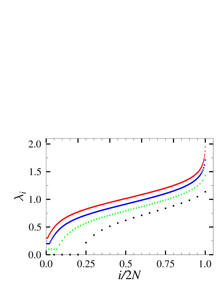
FIG. 1.: Lyapunov spectra for $N=10$ (squares), $N=30$ (diamonds), $N=100$ (circles) and $N=300$ (triangles) in units of $(E/Nma^{2})^{1/2}$. The last three spectra are shifted by 0.1, 0.2 and 0.3$(E/Nma^{2})^{1/2}$, respectively.

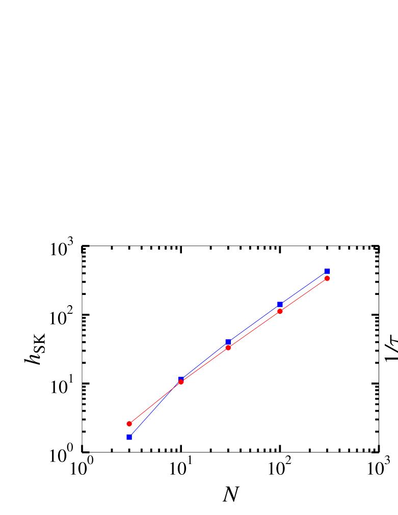
FIG. 2.: KS entropy $h_{\rm SK}$ (squares) and collision rate $1/\tau$ (circles) in units of $(E/Nma^{2})^{1/2}$ as a function of system size $N$.

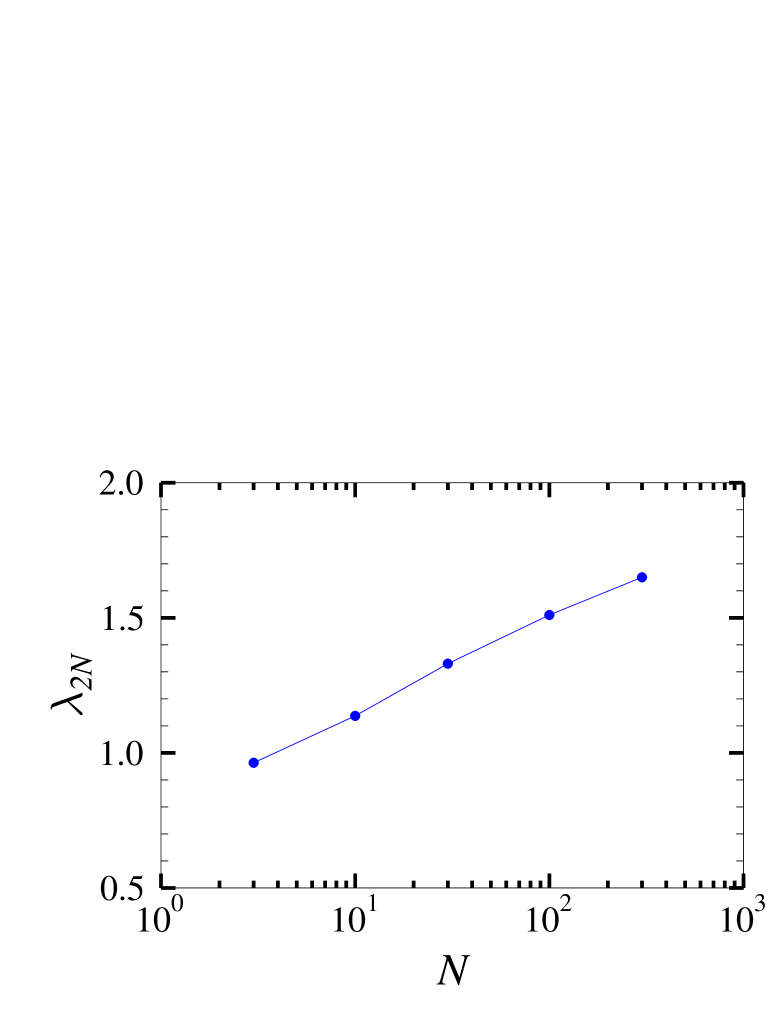
FIG. 3.: Maximal Lyapunov exponent $\lambda_{2N}$ (in units of $(E/Nma^{2})^{1/2}$) as a function of the system size $N$.

REFERENCES

- [1] Ya. G. Sinai, Sov. Math. Dokl. 4, 1818 (1963)
- [2] L. A. Bunimovich, Funct. Anal. Appl. 8, 254 (1974)
- [3] L. A. Bunimovich and J. Rehacek, Commun. Math. Phys. 189, 729 (1997)
- [4] L. Bunimovich, G. Casati, and I. Guarneri, Phys. Rev. Lett.77, 2941 (1996)
- [5] T. Guhr, A. Müller-Groeling, and H. A. Weidenmüller, Phys. Rep. 299, 189 (1998)
- [6] P. Gaspard, Chaos, Scattering and Statistical Mechanics, Cambridge University Press (Cambridge, 1998)
- [7] Ch. Dellago, H. A. Posch, and W. G. Hoover, Phys. Rev. E53 1485, (1996)
- [8] R. van Zon, H. van Beijeren, and J. R. Dorfman, e-print chao-dyn/9906040
- [9] T. Papenbrock, e-print chao-dyn/9905007
- [10] T. Papenbrock and T. Prosen, e-print chao-dyn/9905008
- [11] J.-P. Eckmann and D. Ruelle, Rev. Mod. Phys. 57, 617 (1985)
- [12] L. A. Bunimovich, Chaos 1, 187 (1991)
- [13] G. F. Bertsch, T. Papenbrock, and S. Reddy, e-print nucl-th/9906054
- [14] For a review see e.g. K. D. Luks and J. J. Kozak, Adv. Chem. Phys. 37, 139 (1978)
- [15] T. Prosen (private communication)
- [16] A. J. Lichtenberg and M. A. Lieberman, Regular and Stochastic Motion, Springer-Verlag, (New York 1983)
- [17] L. E. Reichl, The Transition to Chaos in Conservative Classical Systems: Quantum Manifestations, Springer-Verlag, (New York, 1992)
- [18] G. Benettin, L. Galgani, and J. M. Strelcyn, Phys. Rev. A14, 2338 (1976)
- [19] G. Benettin, C. Froeschle, and J. P. Scheidecker, Phys. Rev. A19, 2454 (1979)
- [20] M. Sieber, Nonlinearity 11, 1607 (1998)
- [21] Ya. G. Piesin, Math. Dokl. 17, 196 (1976)
- [22] H. A. Posch and W. G. Hoover, Phys. Rev. A38, 473 (1994)
- [23] R. Livi, A. Politi, and S. Ruffo, J. Phys. A 19, 2033 (1986)
- [24] R. van Zon, H. van Beijeren, and Ch. Dellago, Phys. Rev. Lett.80, 2035 (1998)