Uniform approximations for non-generic bifurcation scenarios including bifurcations of ghost orbits

Abstract

Gutzwiller’s trace formula allows interpreting the density of states of a classically chaotic quantum system in terms of classical periodic orbits. It diverges when periodic orbits undergo bifurcations, and must be replaced with a uniform approximation in the vicinity of the bifurcations. As a characteristic feature, these approximations require the inclusion of complex “ghost orbits”. By studying an example taken from the Diamagnetic Kepler Problem, viz. the period-quadrupling of the balloon-orbit, we demonstrate that these ghost orbits themselves can undergo bifurcations, giving rise to non-generic complicated bifurcation scenarios. We extend classical normal form theory so as to yield analytic descriptions of both bifurcations of real orbits and ghost orbit bifurcations. We then show how the normal form serves to obtain a uniform approximation taking the ghost orbit bifurcation into account. We find that the ghost bifurcation produces signatures in the semiclassical spectrum in much the same way as a bifurcation of real orbits does.

1 Introduction

In the “old” quantum theory developed around the turn of the century, quantization of a mechanical system used to be based on its classical behavior. In 1917, Einstein [7] was able to formulate the quantization conditions found by Bohr and Sommerfeld in their most general form. At the same time, however, Einstein pointed out that they were applicable only to systems whose classical phase space was foliated into invariant tori, i.e., which possess sufficiently many constants of motion, and that most mechanical systems do not meet this requirement. The development of quantum mechanics by Schrödinger, Heisenberg and others then offered techniques which allowed for a precise description of atomic systems without recourse to classical mechanics. Thus, the problem of quantizing chaotic mechanical systems on the basis of their classical behavior remained open.

As late as in the 1960s, Gutzwiller returned to what is now known as a semiclassical treatment of quantum systems. Starting from Feynman’s path integral formulation of quantum mechanics, he derived a semiclassical approximation to the Green’s function of a quantum system which he then used to evaluate the density of states. His trace formula [14, 16] is the only general tool known today for a semiclassical understanding of systems whose classical counterparts exhibit chaotic behavior. It represents the quantum density of states as a sum of a smooth average part and fluctuations arising from all periodic orbits of the classical system, and therefore allows structures in the quantum spectrum to be interpreted in terms of classical mechanics. The derivation of the trace formula assumes all periodic orbits of the system to be isolated. Thus, it is most appropriate for a description of completely hyperbolic system, where in some cases it even allows for a semiclassical determination of individual energy levels, as was done, e.g., by Gutzwiller in the case of the Anisotropic Kepler Problem [15]. In generic Hamiltonian systems exhibiting mixed regular-chaotic dynamics, however, bifurcations of periodic orbits can occur. They cause the trace formula to diverge because close to a bifurcation the periodic orbits involved approach each other arbitrarily closely.

This failure can be overcome if all periodic orbits involved in a bifurcation are treated collectively. A first step in this direction was taken by Ozorio de Almeida and Hannay [24] who proposed formulas for the collective contributions which yield finite results at the bifurcation energy but do not correctly reproduce the results of Gutzwiller’s trace formula as the distance from the bifurcation increases. Similarly, Peters, Jaffé and Delos [26] were able to deal with bifurcations of closed orbits arising in the context of the closed-orbit theory of atomic photoionization. To improve these results, Sieber and Schomerus [35, 31, 36] recently derived uniform approximations which interpolate smoothly between Gutzwiller’s isolated-orbits contributions on either side of the bifurcation. Their formulas are applicable to all kinds of period-$m$-tupling bifurcation generic to Hamiltonian systems with two degrees of freedom.

A closer inspection of bifurcation scenarios encountered in practical applications of semiclassical quantization reveals, however, that the uniform approximations applicable to generic codimension-one bifurcations need to be extended to also include bifurcations of higher codimension. Although these non-generic bifurcations cannot directly be observed if only a single control parameter is varied, they can nevertheless produce clear signatures in semiclassical spectra because in their neighborhood two codimension-one bifurcations approach each other, so that all periodic orbits involved in any of the subsequent bifurcations have to be treated collectively. Examples of this situation were studied by Schomerus and Haake [33, 32] as well as by Main and Wunner [20, 21], who applied techniques of catastrophe theory to achieve a collective treatment of complicated bifurcation scenarios.

All uniform approximations discussed so far in the literature require the inclusion of complex “ghost orbits”. At a bifurcation point, new real periodic orbits are born. If, in the energy range where the real orbits do not exist, the search for periodic orbits is extended to the complexified phase space, the orbits about to be born can be found to possess complex predecessors – ghost orbits. As was first shown by Kuś et. al. [18], some of these ghost orbits, whose contributions become exponentially small in the limit of $\hbar\to 0$, have to be included in Gutzwiller’s trace formula. In addition, the construction of uniform approximations requires complete information about the bifurcation scenario, including ghost orbits.

All bifurcation scenarios discussed in the physics literature so far involved bifurcations of real orbits only. However, there is no reason why ghost orbits should not themselves undergo bifurcations in their process of turning real. It is the purpose of this work to demonstrate that ghost orbit bifurcations do indeed occur and have a pronounced effect on semiclassical spectra if they arise as part of a bifurcation scenario of higher codimension. To this end, we present an example taken from the Diamagnetic Kepler Problem. The example we chose appears to be simple: We discuss the period-quadrupling of the balloon orbit, which is one of the shortest periodic orbits in the Diamagnetic Kepler Problem. However, even this simple case turns out to require the inclusion of a ghost orbit bifurcation.

To cope with this new situation, we have to develop a technique which enables us to deal with the occurence of ghost orbits. It turns out that normal form theory allows for a description of real and ghost orbit bifurcations on an equal footing. Consequently, ghost orbit bifurcations are found to contribute to uniform approximations in much the same way as bifurcations of real orbits do, provided that they occur in connection to bifurcations of real orbits as part of a bifurcation scenario of higher codimension. Therefore, we will arive at the conclusion that in generic Hamiltonian systems with mixed regular-chaotic dynamics the occurence of ghost orbit bifurcations will not be a very exotic, but rather quite a common phenomenon.

The organization of this paper is as follows: In section 2, we briefly summarize the derivation of Gutzwiller’s trace formula, which forms the basis of semiclassical theories of the density of states. Section 3 presents the bifurcation scenario of the example chosen. In section 4, we discuss normal form theory and show that it allows for an analytic description of the example bifurcation scenario. Section 5 then contains the uniform approximation pertinent to the example scenario. It is evaluated in two different degrees of approximation, one of which asymptotically yields perfect agreement with the results of Gutzwiller’s trace formula. A more concise presentation of our main results can be found in [4].

2 Gutzwiller’s trace formula

Gutzwiller’s trace formula offers a way to calculate a semiclassical approximation to the quantum mechanical density of states

$$d(E)=\sum_{j}\delta(E-E_{j})\;,$$ (1)

where the sum extends over all quantum eigenenergies $E_{j}$ of the system under study. In quantum mechanics, the density of states is given by

$$d(E)=\sum_{j}\delta(E-E_{j})=-\frac{1}{\pi}\,{\rm Im}\,\operatorname{Tr}G\;,$$ (2)

where

$$\operatorname{Tr}G:=\int d^{n}x\,G({\bf x}{\bf x},E)\;,$$

and the Green’s function $G({\bf x}^{\prime}{\bf x},E)$ is the configuration space representation of the resolvent operator

$$\hat{G}(E)=(E-\hat{H})^{-1}\;.$$

On the other hand, it is connected to the time-domain propagator $K({\bf x}^{\prime}t^{\prime},{\bf x}t)$ by a Fourier transform

$$G({\bf x}^{\prime}{\bf x},E)=\frac{1}{i\hbar}\int_{0}^{\infty}dt\,K({\bf x}^{\prime}t^{\prime},{\bf x}t)\exp\left\{i\frac{Et}{\hbar}\right\}\;.$$ (3)

Thus, if Feynman’s path integral representation of the propagator

$$K({\bf x}^{\prime}t^{\prime},{\bf x}t)=\int{\cal D}\left({\bf x}(t)\right)\,\exp\left\{\frac{i}{\hbar}\int_{t}^{t^{\prime}}dt\,L\left({\bf x}(t),\dot{{\bf x}}(t),t\right)\right\}$$ (4)

and the Fourier integral are approximately evaluated by the method of stationary phase, one obtains the semiclassical Green’s function ([12], see also [34])

$$G_{scl}({\bf x}^{\prime}{\bf x},E)=\frac{2\pi}{(2\pi i\hbar)^{(n+1)/2}}\sum_{\text{class.traj.}}\sqrt{|D|}\exp\left\{i\left(\frac{S}{\hbar}-\mu\frac{\pi}{2}\right)\right\}\;.$$ (5)

Here, the sum extends over all classical trajectories connecting ${\bf x}$ to ${\bf x}^{\prime}$ at energy $E$,

$$S({\bf x}^{\prime}{\bf x},E)=\int{\bf p}\cdot d{\bf x}$$ (6)

denotes the classical action along the trajectory,

$$D=\det\begin{pmatrix}\frac{\partial^{2}S}{\partial{\bf x}^{\prime}\partial{\bf x}}&\frac{\partial^{2}S}{\partial{\bf x}^{\prime}\partial E}\\[4.30554pt] \frac{\partial^{2}S}{\partial E\partial{\bf x}}&\frac{\partial^{2}S}{\partial E^{2}}\end{pmatrix}\;,$$

and the integer $\mu$ counts the number of caustics the trajectory touches.

To find the density of states, one has to calculate the trace of the semiclassical Green’s function. To this end, one calculates the limit of $G_{scl}$ for ${\bf x}^{\prime}\to{\bf x}$ and then integrate over ${\bf x}$. If ${\bf x}^{\prime}$ is very close to ${\bf x}$, there always exists a direct path connecting ${\bf x}$ to ${\bf x}^{\prime}$. In addition, there are usually indirect paths which leave the neighborhood of their starting point before returning there. The contribution of the direct path can be shown to yield Weyl’s density of states

$$\begin{split}\bar{d}(E)&=\frac{1}{(2\pi\hbar)^{n}}\int d^{n}x\,d^{n}p\,\delta\left(E-\frac{{\bf p}^{2}}{2m}-V({\bf x})\right)\\ &=\frac{1}{(2\pi\hbar)^{n}}\frac{d}{dE}\underbrace{\int d^{n}x\,d^{n}p\,\Theta\left(E-\frac{{\bf p}^{2}}{2m}-V({\bf x})\right)\;,}_{\text{classically accessible volume of phase space}}\end{split}$$ (7)

where $\Theta$ denotes Heaviside’s step function. This result reproduces the well-known fact from statistical mechanics that on the average there is one quantum state per phase space volume of $(2\pi\hbar)^{n}$. The contributions of indirect paths then superimpose system-specific modulations on this general average value.

Due to the stationary-phase condition, only periodic orbits contribute to the semiclassical density of states. To determine the contribution of a single periodic orbit, one introduces a coordinate system with one coordinate running along the periodic orbit and all other coordinates perpendicular to it. Assuming all periodic orbits to be isolated in phase space, one can then evaluate the trace by the method of stationary phase and obtains Gutzwiller’s trace formula for the system-specific modulations of the density of states

$$d^{\prime}(E)=\frac{1}{\pi\hbar}\,{\rm Re}\,\sum_{\text{po}}\frac{T_{0}}{\sqrt{\left|\det(M-I)\right|}}\exp\left\{\frac{i}{\hbar}S-i\frac{\pi}{2}\nu\right\}\;.$$ (8)

Here, the sum runs over all periodic orbits at energy $E$, $S$ denotes the action of the orbit, $T_{0}$ its primitive period, $M$ its monodromy matrix, which describes the stability of the orbit, and $\nu$ its Maslov index, which reflects the topology of nearby orbits. In the derivation, the primitive period $T_{0}$ can be seen to arise from the integration along the orbit, whereas the occurrence of the monodromy matrix is due to the integrations over the transverse coordinates.

Gutzwiller’s trace formula expresses the quantum density of states in terms of purely classical data. It fails, however, if the periodic orbits of the classical system cannot be regarded as isolated, as is the case, e.g., close to a bifurcation. There, the failure of the trace formula manifests itself in a divergence of the isolated-orbits contributions in (8): If an orbit undergoes a bifurcation, the determinant of $M-I$ vanishes. In recent years, the problem of calculating the joint contribution of bifurcating orbits to the density of states was addressed by various authors, whose works were briefly reviewed in the introduction. It is the purpose of the present paper to present normal form theory as a technique which allows one to achieve a collective description of bifurcating orbits and to show its applicability to a complicated bifurcation scenario. In particular, we shall demonstrate that bifurcations of ghost orbits need to be included in the description of classical bifurcation scenarios because they can exert a marked influence on semiclassical spectra, and that classical normal form theory can be extended so as to meet this requirement. However, before we come to deal with the construction of uniform approximations in sections 4 and 5, we shall give a description of our example system, the Diamagnetic Kepler Problem, and the bifurcation scenario we are going to study.

3 The Diamagnetic Kepler Problem

3.1 The Hamiltonian

As a prototype example of a system which undergoes a transition to chaos, we shall investigate the hydrogen atom in a homogeneous external magnetic field, which is reviewed, e.g., in [9, 17, 38]. We assume the nucleus fixed and regard the electron as a structureless point charge moving under the combined influences of the electrostatic Coulomb force and the Lorentz force. Throughout this paper, we shall use atomic units, let the magnetic field point along the $z$-direction and denote its strength by $\gamma=B/B_{0}$, where $B_{0}=m^{2}e^{3}(4\pi\varepsilon_{0})^{-2}\hbar^{-3}=2.3505\cdot 10^{5}\rm T$ is the atomic unit of the magnetic field strength. The Hamiltonian then reads

$$H=\frac{{\bf p}^{\,2}}{2}+\frac{\gamma}{2}L_{z}+\frac{\gamma^{2}}{8}\left(x^{2}+y^{2}\right)-\frac{1}{r}\;,$$ (9)

where $r=|{\bf x}|$ and $L_{z}={\bf e}_{z}\cdot\left({\bf x}\times{\bf p}\right)$ denotes the $z$-component of the angular momentum. In the following, we will restrict ourselves to the case $L_{z}=0$. As a consequence, the angular coordinate $\varphi$ measuring rotation around the field axis becomes ignorable, so that we are effectively dealing with a two-degree-of-freedom system.

The energy $E=H$ is a constant of motion. Thus, the dynamics depends on both the energy and the magnetic field strength as control parameters. This situation can be simplified, however, if one exploits the scaling properties of the Hamiltonian. If classical quantities are scaled according to

$$\begin{array}[]{r@{}l@{}l@{\qquad\qquad}r@{}l@{}l}{\bf x}&\mapsto\tilde{{\bf x}}&=\gamma^{2/3}{\bf x}\;,&{\bf p}&\mapsto\tilde{{\bf p}}&=\gamma^{-1/3}{\bf p}\;,\\ H&\mapsto\tilde{H}&=\gamma^{-2/3}H\;,&t&\mapsto\tilde{t}&=\gamma t\;,\\ S&\mapsto\tilde{S}&=\gamma^{1/3}S\;,\end{array}$$ (10)

one obtains the scaled Hamiltonian

$$\begin{split}\tilde{H}&=\frac{\tilde{{\bf p}}^{2}}{2}+\frac{1}{8}\left(\tilde{x}^{2}+\tilde{y}^{2}\right)-\frac{1}{\tilde{r}}\\ &=\tilde{E}=\gamma^{-2/3}E\;.\end{split}$$ (11)

The scaled dynamics depends on the scaled energy as its only control parameter.

The equations of motion following from this Hamiltonian are difficult to handle numerically due to the Coulomb singularity at $\tilde{r}=0$. To overcome this problem, one introduces semiparabolical coordinates

$$\mu^{2}=\tilde{r}-\tilde{z}\;,\qquad\qquad\nu^{2}=\tilde{r}+\tilde{z}$$ (12)

and a new orbital parameter $\tau$ defined by

$$dt=2r\,d\tau=\left(\mu^{2}+\nu^{2}\right)\,d\tau\;.$$

These transformations lead to the final form of the Hamiltonian

$${\cal H}=\frac{p_{\mu}^{2}+p_{\nu}^{2}}{2}-\tilde{E}\left(\mu^{2}+\nu^{2}\right)+\frac{1}{8}\mu^{2}\nu^{2}\left(\mu^{2}+\nu^{2}\right)\equiv 2\;.$$ (13)

In this form, the scaled energy $\tilde{E}$ plays the rôle of an external parameter, whereas the value of the Hamiltonian is fixed: It has to be chosen equal to 2. The equations of motion following from this Hamiltonian do not contain singularities any more so that they can easily be integrated numerically.

Note that the definition (12) determines the semiparabolical coordinates up to a choice of sign only. Thus, orbits which are mirror images of each other with respect to a reflection at the $\mu$- or $\nu$-axes have to be identified. Furthermore, if we follow a periodic orbit until it closes in $(\mu,\nu)$-coordinates, this may correspond to more than one period in the original configuration space. This has to be kept in mind when interpreting plots of periodic orbits in semiparabolical coordinates.

As a substantial extension of the classical description of the Diamagnetic Kepler Problem we complexify the classical phase space by allowing coordinates and momenta to assume complex values. As the Hamiltonian (13) is holomorphic, we can at the same time regard the phase space trajectories as functions of complex times $\tau$. To numerically calculate the solution of the equations of motion at a given time $\tau_{f}$, we integrate the equations of motion along a path connecting the origin of the complex $\tau$-plane to the desired endpoint $\tau_{f}$. By Cauchy’s integral theorem, the result does not depend on the path chosen so that we can safely choose to integrate along a straight line from $0$ to $\tau_{f}$. This extension allows us to look for ghost orbit predecessors of real periodic orbits born in a bifurcation. In general, their orbital parameters $S$, $T$ and the monodromy matrix $M$ will be complex. We calculate them along with the numerical integration of the equations of motion from

$$T=\int_{0}^{\tau_{f}}(\mu^{2}+\nu^{2})\,d\tau\;,\qquad S=\int_{0}^{\tau_{f}}(p_{\mu}^{2}+p_{\nu}^{2})\,d\tau\;.$$

3.2 The bifurcation scenario

The Diamagnetic Kepler Problem described by the Hamiltonian (13) exhibits a transition between regular dynamics at strongly negative scaled energies $\tilde{E}\to-\infty$ and chaotic dynamics at $\tilde{E}\approx 0$ and above (for details see, e.g., [17]). Correspondingly, there are only three different periodic orbits at very low scaled energy, whereas the number of periodic orbits increases exponentially as $\tilde{E}\nearrow 0$.

At any fixed scaled energy, there is a periodic orbit parallel to the magnetic field. It is purely Coulombic since a motion parallel to the magnetic field does not cause a Lorentz force. This orbit is stable at low negative scaled energies; as $\tilde{E}\nearrow 0$, however, it turns unstable and stable again infinitely often [39]. For the first time, instability occurs at $\tilde{E}=-0.391$. In this bifurcation, a stable and an unstable periodic orbit are born. The stable orbit is known as the balloon orbit. It is depicted in figure 1. As shown in bifurcation theory, the stability of a periodic orbit is determinded by the trace of its monodromy matrix. For the balloon orbit, the trace is shown in figure 2. It equals 2 when the orbit is born. As the scaled energy increases, the trace decreases monotonically. The orbit turns unstable at $\tilde{E}=-0.291$, where the trace equals $-2$. In between, all kinds of period-$m$-tupling bifurcations occur. In this work, we shall discuss the period-quadrupling bifurcation which arises at the zero of the trace at $\tilde{E}_{c}=-0.342025$.

For $\tilde{E}>\tilde{E}_{c}$, two real satellite orbits of quadruple period exist. They are depicted in figure 3 at two different values of the scaled energy. The solid and dashed curves in the plots represent the stable and unstable satellite orbits, respectively. In both cases, the balloon orbit is shown for comparison as a dotted curve. The satellites can clearly be seen to approach the balloon orbit as $\tilde{E}\searrow\tilde{E}_{c}$. At $\tilde{E}_{c}$, they collide with the balloon orbit and disappear. Below $\tilde{E}_{c}$, a stable and an unstable ghost satellite exist instead. They are presented as the solid and dotted curves in figure 4. Note that the imaginary parts are small compared to the real parts because the bifurcation where the imaginary parts vanish is close. As the Hamiltonian (13) is real, the complex conjugate of any orbit is again a solution of the equations of motion. In this case, however, the ghost satellites coincide with their complex conjugates, so that the total number of orbits is conserved in the bifurcation. This behavior can be understood in terms of normal form theory (see section 4.2).

The orbits described so far form a generic kind of period-quadrupling bifurcation as described by Meyer [23] and dealt with in the context of semiclassical quantization by Sieber and Schomerus [36]. In our case, however, this description of the bifurcation scenario is not yet complete because there exists an additional periodic ghost orbit at scaled energies around $\tilde{E}_{c}$. Its shape is shown as a dashed curve in figure 4. It is very similar to the stable ghost satellite originating in the period-quadrupling, and indeed, when following the ghost orbits to lower energies, we find another bifurcation at $\tilde{E}_{c}^{\prime}=-0.343605$, i.e., only slightly below the bifurcation point $\tilde{E}_{c}=-0.342025$ of the period-quadrupling. At $\tilde{E}_{c}^{\prime}$, the additional ghost orbit collides with the stable ghost satellite, and these two orbits turn into a pair of complex conjugate ghost orbits. Their shapes are presented at a scaled energy of $\tilde{E}=-0.344$ as the solid and dashed curves in figure 5. From the imaginary parts, the loss of conjugation symmetry can clearly be seen if the symmetries of the semiparabolical coordinate system as described above are taken into account. The dotted curve in figure 5 represents the unstable ghost satellite which was already present at $\tilde{E}>\tilde{E}_{c}^{\prime}$. It does not undergo any further bifurcations.

Note that the second bifurcation at $\tilde{E}=\tilde{E}_{c}^{\prime}$ involves ghost orbits only. This kind of bifurcation has not yet been described in the literature so far. In particular, Meyer’s classification of codimension-one bifurcations in generic Hamiltonian systems covers bifurcations of real orbits only and does not include bifurcations of ghost orbits. Consequently, the influence of ghost orbit bifurcations on semiclassical spectra has never been investigated so far. Due to the existence of this bifurcation, however, the results by Sieber and Schomerus [36] concerning generic period-quadrupling bifurcations cannot be applied to the complicated bifurcation scenario described here. As in cases dealt with before by Main and Wunner [20, 21] as well as by Schomerus and Haake [31, 33], who discussed the semiclassical treatment of two neighboring bifurcations of real orbits, the closeness of the two bifurcations requires the construction of a uniform approximation taking into account all orbits involved in either bifurcation collectively. Thus, the ghost orbit bifurcation at $\tilde{E}_{c}^{\prime}$ turns out to contribute to the semiclassical spectrum in much the same way as a bifurcation of real orbits does, as long as we do not go to the extreme semiclassical domain where the two bifurcations can be regarded as isolated and ghost orbit contributions vanish altogether.

To construct a uniform approximation, we need to know the periodic orbit parameters of all orbits involved in the bifurcations. The parameters were calculated numerically and are displayed in figure 6 as functions of the scaled energy. Part (a) of this figure presents the actions of the orbits. To exhibit the sequence of bifurcations more clearly, the action of four repetitions of the central balloon orbit was chosen as a reference level $(\Delta S=0)$. Around $\tilde{E}_{c}$, we recognize two almost parabolic curves which indicate the actions of the stable (upper curve) and unstable (lower curve) satellite orbits. At $\tilde{E}_{c}$, the curves change from solid to dashed as the satellite orbits become complex. Another dashed line represents the action of the additional ghost orbit, which can clearly be seen not to collide with the balloon orbit at $\tilde{E}_{c}$. Whereas the unstable ghost satellite does not undergo any further bifurcations, the curves representing the stable and the additional ghost orbits can be seen to join at $\tilde{E}_{c}^{\prime}=-0.343605$. Below $\tilde{E}_{c}^{\prime}$, a dotted curve indicates the presence of a pair of complex conjugate ghosts. The imaginary parts of their actions are different from zero and have opposite signs, whereas above $\tilde{E}_{c}^{\prime}$, all ghost orbits coincide with their complex conjugates so that their actions are real.

Analogously, part (b) of figure 6 presents the orbital periods. In this case, no differences were taken, so that the period of the fourth repetition of the balloon orbit, which is always real, appears in the figure as a nearly horizontal line at $T\approx 5.84$. The other orbits can be identified with the help of the bifurcations they undergo, similar to the discussion of the actions given above. Finally, figure 6(c) shows the traces of the monodromy matrices minus two. For Hamiltonian systems with two degrees of freedom, these quantities agree with $\det(M-I)$. At $\tilde{E}_{c}$ and $\tilde{E}_{c}^{\prime}$, they can be seen to vanish for the bifurcating orbits, thus causing the periodic orbit amplitudes (8) to diverge at the bifurcation points.

4 Normal form theory and bifurcations

4.1 Birkhoff-Gustavson normal form

As we have seen, Gutzwiller’s trace formula (8) fails close to bifurcations, when periodic orbits of the classical system cannot be regarded as isolated. To overcome this difficulty, we need a technique which allows us to describe the structure of the classical phase space close to a bifurcating orbit. This can be done with the help of normal form theory. A detailed description of this technique can be found in [1, Appendix 7] or [25, Sections 2.5 and 4.2]. Here, we will present the normal form transformations for systems with two degrees of freedom only, although the general scheme is the same for higher dimensional cases. As only stable periodic orbits can undergo bifurcations, we will restrict ourselves to this case.

As a first step, we introduce a special canonical coordinate system $(\vartheta,p_{\vartheta},q,p)$ in a neighborhood of a periodic orbit, which has the following properties (concerning the existence of such a coordinate system, see [2, Chapter 7.4, Proposition 1]):

• $\vartheta$ is measured along the periodic orbit and $q$ perpedicular to it, so that phase space points lying on the periodic orbit are characterized by $q=p=0$.

• $\vartheta$ assumes values between 0 and $2\pi$, and along the periodic orbit we have, up to a constant,

  $$\vartheta=\frac{2\pi}{T}t\;,$$

  where $T$ denotes the orbital period.

• If we choose an initial condition in the neighborhood and $0\leq\vartheta<T$, the function $\vartheta(t)$ is invertible.

According to the last condition, we can regard $p$ and $q$ as functions of $\vartheta$ instead of $t$.

The classical dynamics of a mechanical system is given by Hamilton’s variational principle, which states that a classical trajectory with fixed initial and final coordinates ${\bf q}(t_{1})$ and ${\bf q}(t_{2})$ satisfies

$$\delta\,\int_{\left({\bf q}(t_{1}),t_{1}\right)}^{\left({\bf q}(t_{2}),t_{2}\right)}{\bf p}\cdot d{\bf q}-H\,dt=0\;.$$ (14)

If we restrict ourselves to considering the energy surface given by a fixed energy $E$, we can transform the integral as follows:

$$\begin{split}\int{\bf p}\cdot d{\bf q}-H\,dt&=\int p\,dq+p_{\vartheta}\,d\vartheta-H\,dt\\ &=\int p\,dq-(-p_{\vartheta})\,d\vartheta\quad-E(t_{2}-t_{1})\;.\end{split}$$ (15)

The last term in this expression is a constant which does not contribute to the variation of the integral, so that actual orbits of the system satisfy

$$\delta\!\int p\,dq-(-p_{\vartheta})\,d\vartheta\;=\;\delta\!\int{\bf p}\cdot d{\bf q}-H\,dt\;=\;0\;.$$ (16)

Thus, the dependence of $p$ and $q$ on the new parameter $\vartheta$ is given by Hamilton’s equations of motion, where $-p_{\vartheta}$ plays the rôle of the Hamiltonian. It has to be determined as a function of the new phase space coordinates $p,q$, the ”time” $\vartheta$ and the energy $E$, which occurs as a parameter, from the equation

$$H\left(\vartheta,p_{\vartheta},q,p\right)=E$$

From our choice of the coordinate system, $p_{\vartheta}$ is periodic in $\vartheta$ with a period of $2\pi$.

We have now reduced the dynamics of a two-degrees-of-freedom autonomous Hamiltonian system to that of a single-degree-of-freedom system, which is, however, no longer autonomous, but periodically time-dependent. With regard to the original system, we can view the motion perpendicular to the periodic orbit as being periodically driven by the motion along the orbit. Henceforth, we shall denote the Hamiltonian of the reduced system by $\Phi$, coordinate and momentum by $q$ and $p$, respectively, and the time by $\vartheta$.

The point $p=q=0$ corresponds to the periodic orbit of the original system and therefore constitutes a stable equilibrium position of the reduced system so that a Taylor series expansion of the Hamiltonian around this point does not have linear terms. By a suitable time-dependent canonical transformation, the quadratic term can be made time-independent, see [29]. We expand the Hamiltonian in a Taylor series in $p$ and $q$ and in a Fourier series in $\vartheta$:

$$\Phi(p,q,\vartheta)=\frac{\omega}{2}(p^{2}+q^{2})+\sum_{\alpha+\beta=3}^{\infty}\sum_{l=-\infty}^{\infty}\Phi_{\alpha\beta l}p^{\alpha}q^{\beta}\exp(il\vartheta)\;.$$ (17)

To go on, we introduce complex coordinates

$$z=p+iq\qquad\qquad z^{\ast}=p-iq\;.$$

This transformation is canonical with multiplier $-2i$, so that we have to go over to a new Hamiltonian

$$\begin{split}\phi&=-2i\Phi\\ &=-i\omega zz^{\ast}+\sum_{\alpha+\beta=3}^{\infty}\sum_{l=-\infty}^{\infty}\phi_{\alpha\beta l}z^{\alpha}z^{\ast\beta}\exp(il\vartheta)\end{split}$$ (18)

Birkhoff [5, Chapter 3] and Gustavson [11] developed a technique which allows us to systematically eliminate low-order terms from this expansion by a sequence of canonical transformations. To eliminate terms of order $\alpha+\beta=k$, we employ the transformation given by the generating function

$${\cal F}_{2}(Z^{\ast},z,\vartheta)=-zZ^{\ast}-\sum_{\alpha+\beta=k}\sum_{l=-\infty}^{\infty}{\cal F}_{\alpha\beta l}z^{\alpha}Z^{\ast\beta}\exp(il\vartheta)$$ (19)

with arbitrary expansion coefficients ${\cal F}_{\alpha\beta l}$, so that the transformation reads

$$Z=-\frac{\partial{\cal F}_{2}}{\partial Z^{\ast}} =z\left(1+\sum\beta{\cal F}_{\alpha\beta l}z^{\alpha-1}Z^{\ast\beta-1}\exp(il\vartheta)\right)\;,$$ (20)

$$z^{\ast}=-\frac{\partial{\cal F}_{2}}{\partial z} =Z^{\ast}\left(1+\sum\alpha{\cal F}_{\alpha\beta l}z^{\alpha-1}Z^{\ast\beta-1}\exp(il\vartheta)\right)\;,$$

if the new coordinates are denoted by $Z$ and $Z^{\ast}$. From these equations, we have

$$\begin{split}z&=Z-\sum\beta{\cal F}_{\alpha\beta l}z^{\alpha-1}ZZ^{\ast\beta-1}\exp(il\vartheta)+\dots\;,\end{split}$$ (21)

so that

$$zz^{\ast}=ZZ^{\ast}+\sum(\alpha-\beta){\cal F}_{\alpha\beta l}Z^{\alpha}Z^{\ast\beta}\exp(il\vartheta)+\dots\;,$$ (22)

where the dots indicate terms of order higher than $k$.

For the new Hamiltonian we find

$$\begin{split}\phi^{\prime}&=\phi-\frac{\partial{\cal F}_{2}}{\partial t}\\ &=\begin{aligned} -i\omega zz^{\ast}&+\text{terms of order $<k$}\\ &+\sum_{\stackrel{{\scriptstyle\alpha+\beta=k}}{{l}}}\left\{\phi_{\alpha\beta l}z^{\alpha}z^{\ast\beta}+il{\cal F}_{\alpha\beta l}z^{\alpha}Z^{\beta}\right\}\exp(il\vartheta)\\ &+\text{higher-order terms}\end{aligned}\\ &=\begin{aligned} -i\omega ZZ^{\ast}&-i\omega\sum(\alpha-\beta){\cal F}_{\alpha\beta l}Z^{\alpha}Z^{\ast\beta}\exp(il\vartheta)\\ &+\text{terms of order $<k$}\\ &+\sum\left\{\phi_{\alpha\beta l}+il{\cal F}_{\alpha\beta l}\right\}Z^{\alpha}Z^{\ast\beta}\exp(il\vartheta)\\ &+\text{higher-order terms}\end{aligned}\\ &=\begin{aligned} -i\omega ZZ^{\ast}&+\text{terms of order $<k$}\\ &-i\sum\left\{\left(\omega(\alpha-\beta)-l\right){\cal F}_{\alpha\beta l}+i\phi_{\alpha\beta l}\right\}Z^{\alpha}Z^{\ast\beta}\exp(il\vartheta)\\ &+\text{higher-order terms}\;.\end{aligned}\end{split}$$ (23)

Thus, terms of order less than $k$ remain unchanged during the transformation, whereas if we choose

$${\cal F}_{\alpha\beta l}=-\frac{i\phi_{\alpha\beta l}}{\omega(\alpha-\beta)-l}\;,$$ (24)

the term $(\alpha\beta l)$ in (19) cancels the term $(\alpha\beta l)$ in the expansion of the Hamiltonian. Therefore, we can successively eliminate terms of ever higher order without destroying the simplifications once achieved in later steps.

Of course, the generating function (19) must not contain terms that make the denominator in (24) vanish. Thus, we cannot eliminate resonant terms satisfying $\omega(\alpha-\beta)-l=0$. If $\omega$ is irrational, only terms having $\alpha=\beta$ and $l=0$ are resonant, so that we can transform the Hamiltonian (18) to the form

$$\phi=-i\omega zz^{\ast}+\phi_{2}(zz^{\ast})^{2}+\dots+\phi_{k}(zz^{\ast})^{[k/2]}+{\cal O}((z+z^{\ast})^{k+1})$$ (25)

with arbitrarily large $k$.

If $\omega$ is rational, however, further resonant terms occur, so that the normal form will become more complicated then (25). These additional terms must also be kept if we want to study the behavior of the system close to a resonance. So, let $\omega\!\approx\!\frac{n}{m}$ with coprime integers $n$ and $m$, so that the resonance condition $\omega(\alpha-\beta)-l=0$ reads

$$n(\alpha-\beta)=ml$$ (26)

and time-dependent resonant terms with $l\neq 0$ occur. This time-dependence can be abandoned, if we transform to a rotating coordinate system

$$Z=z\exp(in\vartheta/m)\;,\qquad\qquad Z^{\ast}=z^{\ast}\exp(-in\vartheta/m)\;,$$ (27)

This transformation, which is generated by

$${\cal F}_{2}=-Z^{\ast}z\exp(in\vartheta/m)\;,$$

changes resonant terms according to

$$\begin{split}z^{\alpha}z^{\ast\beta}\exp(il\vartheta)&=Z^{\alpha}\exp(-in\vartheta\alpha/m)Z^{\ast\beta}\exp(in\vartheta\beta/m)\exp(il\vartheta)\\ &=Z^{\alpha}Z^{\ast\beta}\exp(-i\{n(\alpha-\beta)-ml\}\vartheta/m)\\ &=Z^{\alpha}Z^{\ast\beta}\;.\end{split}$$

Thus, all resonant terms become time-independent, whereas non-resonant terms acquire a time-dependence with period $2\pi m$. The Hamiltonian is transformed as

$$\begin{split}\phi^{\prime}&=\phi-\frac{\partial{\cal F}_{2}}{\partial t}\\ &=\phi+i\frac{n}{m}Z^{\ast}z\exp(int/m)\\ &=\phi+i\frac{n}{m}ZZ^{\ast}\\ &=\begin{aligned} -i\left(\omega-\frac{n}{m}\right)ZZ^{\ast}&+\phi_{2}(ZZ^{\ast})^{2}+\dots\\ &+\text{further resonant terms}\\ &+\text{non-resonant terms of higher order}\;,\end{aligned}\end{split}$$

that is, in the harmonic part of the Hamiltonian the frequency $\omega$ is replaced by a small parameter $2\varepsilon=\omega-\frac{n}{m}$ measuring the distance from the resonance.

As we are looking for a local description of the system in a neighborhood of the equilibrium position $z=z^{\ast}=0$, we can abort the normal form transformation at a suitable $k$ and neglect higher-order terms. This way, we get an “idealized” Hamiltonian that quantitatively approximates the actual Hamiltonian close to the equilibrium.

At the end, we return to the original coordinates $p$, $q$ or to action-angle-coordinates $(I,\varphi)$ given by

$$p =\sqrt{2I}\cos\varphi\;, q =\sqrt{2I}\sin\varphi\;,$$

$$z =\sqrt{2I}\exp(i\varphi)\;, z^{\ast} =\sqrt{2I}\exp(-i\varphi)\;,$$ (28)

$$I =\frac{1}{2}(p^{2}+q^{2})=\frac{1}{2}zz^{\ast}\;.$$

We have thus obtained a selection of the most important low-order terms that determine the behavior of the system close to the central periodic orbit.

According to the resonance condition (26) and as $n$ and $m$ are coprime, for all resonant terms $\alpha-\beta=rm,r\in\mathbb{Z}$, is a multiple of $m$, so that a resonant term has the form

$$\begin{split}z^{\alpha}z^{\ast\beta}&=\left(\sqrt{2I}\right)^{\alpha+\beta}\exp\left\{i(\alpha-\beta)\varphi\right\}\\ &=\left(\sqrt{2I}\right)^{k}\exp\left\{irm\varphi\right\}\end{split}$$

and is periodic in $\varphi$ with a period of $\frac{2\pi}{m}$. Thus, although we started from a generic Hamiltonian, the normal form exhibits $m$-fold rotational symmetry in a suitably chosen coordinate system. Furthermore, all resonant terms satisfy

$$|rm|=|\alpha-\beta|\leq\alpha+\beta=k\;,$$

$$\alpha=\frac{1}{2}(k+rm)\in\mathbb{Z}\;,$$

$$\beta=\frac{1}{2}(k-rm)\in\mathbb{Z}\;.$$

Thus, the normal form reads

$$\Phi=\sum_{k}c_{k}I^{k}+\sum_{k}\sum_{\stackrel{{\scriptstyle 0<rm\leq k}}{{k\pm rm\text{ even}}}}\sqrt{I}^{\,k}\Big{[}d_{k}\cos(rm\varphi)+d_{k}^{\prime}\sin(rm\varphi)\Big{]}\;.$$ (29)

As this Hamiltonian is time-independent, it is an (approximate) constant of motion, so that all points an orbit with given initial conditions can reach lie on a level line of the Hamiltonian. Thus, a contour plot of the Hamiltonian will exhibit lines one will also find in a Poincaré surface of section of the original Hamiltonian system.

As an example and to describe the bifurcation scenario presented in Section 3, we will now discuss the case of a fourth-order resonance $m=4$. Up to the sixth order, the following terms turn out to be resonant:

$$\phi= -i\left(\omega-\frac{n}{4}\right)zz^{\ast} 2$$ order

$$+\phi_{2}(zz^{\ast})^{2}+\phi_{4,0,n}z^{4}+\phi_{0,4,-n}z^{\ast 4} 4$$ (30)

$$+\phi_{3}(zz^{\ast})^{3}+\phi_{5,1,n}z^{5}z^{\ast}+\phi_{1,5,-n}zz^{\ast 5}\;,\qquad 6$$

so that the real normal form reads

$$\begin{split}\Phi=\quad&\varepsilon I\\ +&aI^{2}+bI^{2}\cos(4\varphi)+b^{\prime}I^{2}\sin(4\varphi)\\ +&cI^{3}+dI^{3}\cos(4\varphi)+eI^{3}\sin(4\varphi)\end{split}$$ (31)

with $\varepsilon=\frac{1}{2}(\omega-\frac{n}{4})$ and suitably chosen real coefficients $a,b,b^{\prime},c,d,e$. The physical meaning of these terms will be discussed in the sequel.

4.2 Generic Bifurcations

To lowest order, the normal form (31) reads

$$\Phi=\varepsilon I=\frac{\varepsilon}{2}(p^{2}+q^{2})\;.$$ (32)

This is a harmonic-oscillator Hamiltonian. It describes orbits which start close to the central periodic orbit and wind around it with frequency $\omega+\varepsilon$, or frequency $\varepsilon$ in the rotating coordinate system.

In second order in $I$, angle-dependent terms in the normal form occur. For arbitrary resonances, the lowest order of the normal form containing this kind of nontrivial terms describes the generic codimension-one bifurcations of periodic orbits as classified by Meyer [23], that is, those kinds of bifurcations that can typically be observed if a single control parameter is varied in a system with two degrees of freedom and without special symmetries. As was shown by Meyer, for any order $m$ of resonance there is only one possible kind of bifurcation, except for the case $m=4$, where there are two. In the sequel, we are going to discuss these possibilities for $m=4$.

Up to second order in $I$, the normal form (31) reads

$$\Phi=\varepsilon I+aI^{2}+bI^{2}\cos(4\varphi)+b^{\prime}I^{2}\sin(4\varphi)\;.$$ (33)

Shifting the angle $\varphi$ according to $\varphi\mapsto\varphi+\varphi_{0}$, we can eliminate the term proportional to $\sin(4\varphi)$, that is, we can assume $b^{\prime}=0$, so that the normal form simplifies to

$$\Phi=\varepsilon I+aI^{2}+bI^{2}\cos(4\varphi)\;.$$ (34)

To find periodic orbits of the system, we have to determine the stationary points of the normal form. The central periodic orbit we expanded the Hamiltonian around is located at $I=0$ and does not show up as a stationary point, because the action-angle-coordinate chart (4.1) is singular there.

For $I\neq 0$, we have

$$0 \stackrel{{\scriptstyle\textstyle!}}{{=}}\frac{\partial\Phi}{\partial\varphi}=-4bI^{2}\sin(4\varphi)\;,$$ (35)

$$0 \stackrel{{\scriptstyle\textstyle!}}{{=}}\frac{\partial\Phi}{\partial I}=\varepsilon+2aI+2bI\cos(4\varphi)\;.$$

From the first of these equations, we get $\sin(4\varphi)=0$, that is, $\cos(4\varphi)=\sigma\equiv\pm 1$. The second equation then yields

$$I_{\sigma}=-\frac{\varepsilon}{2(a+\sigma b)}\;.$$ (36)

For any choice of $\sigma$, there are four different angles $\varphi,0\leq\varphi<2\pi$, satisfying $\sin(4\varphi)=0$ and $\cos(4\varphi)=\sigma$, corresponding to four different stationary points in a Poincaré surface of section. All these stationary points belong to the same periodic orbit, which is four times as long as the central orbit.

For a real periodic orbit, $I=\frac{1}{2}(p^{2}+q^{2})$ is real and positive. Thus, if we get a negative value for $I$ from (36), this indicates a complex periodic orbit. The action of this orbit, which we identify with the stationary value $\Phi(I_{\sigma})$ of the normal form, is real if $I_{\sigma}$ is real. Therefore, if $I_{\sigma}$ is real and negative, we are dealing with a ghost orbit symmetric with respect to complex conjugation. Keeping these interpretations in mind, we find the two possible forms of period-quadrupling bifurcations:

• $|a|>|b|$: Island-Chain-Bifurcation
  In this case, the signs of $a+b$ and $a-b$ are both equal to the sign of $a$. If $\operatorname{sign}\varepsilon=-\operatorname{sign}a$, both solutions $I_{\sigma}$ from equation (36) are positive, if $\operatorname{sign}\varepsilon=\operatorname{sign}a$, they are negative. Thus, on one hand side of the resonance, there are a stable and an unstable real satellite orbit. As $\varepsilon\to 0$, these orbits collapse onto the central periodic orbit and reappear as two complex satellite orbits on the other side of the resonance.

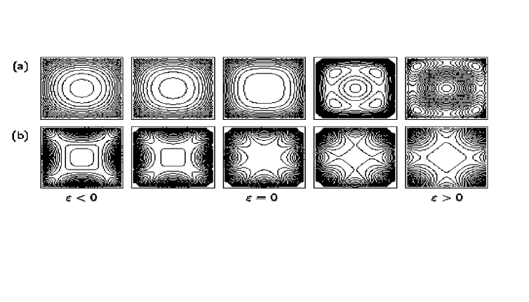
Figure 7: Contour plots of the normal form (34) illustrating the two generic types of period-quadrupling bifurcations. (a) Island-Chain-Bifurcation, (b) Touch-and-Go-Bifurcation.

  Part (a) of figure 7 shows a sequence of contour plots of the normal form, which we interprete as a sequence of Poincaré surface of section plots. If $\varepsilon<0$, we recognize a single elliptic fixed point at the centre of the plots, which corresponds to the stable central orbit. If $\varepsilon>0$, four elliptic and four hyperbolic fixed points appear in addition. They indicate the presence of the real satellite orbits. Due to these plots, the bifurcation encountered here is called an island-chain-bifurcation. It was this kind of bifurcation which we observed in the example of section 3 at energy $E_{c}$.

• $|a|<|b|$: Touch-and-Go-Bifurcation
  In this case, the signs of $a+b$ and $a-b$ are different, that is, at any given $\varepsilon$, there are a real and a complex satellite orbit. As $\varepsilon$ crosses 0, the real satellite becomes complex and vice versa.

  A sequence of contour plots for this case is shown in part (b) of figure 7. At any $\varepsilon$, the central elliptic fixed point is surrounded by four hyperbolic fixed points indicating the presence of an unstable real satellite. At $\varepsilon>0$, the fixed points are located at different angles than at $\varepsilon<0$, that is, it is the orbit with different $\sigma$ which has become real. This kind of bifurcation is known as a touch-and-go-bifurcation.

4.3 Sequences of Bifurcations

In the discussion of a specific Hamiltonian system it can often be observed that the generic bifurcations as described by Meyer occur in organized sequences. Examples of such sequences have been discussed by Mao and Delos [19] for the Diamagnetic Kepler Problem. In the example presented in section 3, we also encountered a sequence of two bifurcations. As Sadovskií, Shaw and Delos were able to show [28, 29], sequences of bifurcations can be described analytically if higher order terms of the normal form expansion are taken into account. In the sequel, we are going to use all terms in the expansion (31) up to third order in $I$. As we did above, we can eliminate the $b^{\prime}$-term if we shift $\varphi$ by a suitably chosen constant, so that the normal form reads:

$$\Phi=\varepsilon I+aI^{2}+bI^{2}\cos(4\varphi)+cI^{3}+dI^{3}\cos(4\varphi)+eI^{3}\sin(4\varphi)\;.$$ (37)

It can be further simplified by canonical transformations, whereby the transformations need to be performed up to third order in $I$ only, as higher terms have been neglected anyway.

As a first step, we apply a canonical transformation to new coordinates $\hat{I}$ and $\hat{\varphi}$ which is generated by the function

$${\cal F}_{2}=-\hat{I}\varphi+\frac{e}{8b}{\hat{I}}^{2}\;,$$ (38)

that is

$$\begin{split}I=-\frac{\partial{\cal F}_{2}}{\partial\varphi}&=\hat{I}\;,\\ \hat{\varphi}=-\frac{\partial{\cal F}_{2}}{\partial\hat{I}}&=\varphi-\frac{e}{4b}\hat{I}\;.\end{split}$$ (39)

Inserting these transformations into the normal form, we obtain up to terms of order $\hat{I}^{4}$:

$$\Phi=\varepsilon\hat{I}+a{\hat{I}}^{2}+b{\hat{I}}^{2}\cos(4\hat{\varphi})+c{\hat{I}}^{3}+d{\hat{I}}^{3}\cos(4\hat{\varphi})\;.$$ (40)

This expression is further simplified by another canonical transformation generated by

$${\cal F}_{2}=-\tilde{I}\hat{\varphi}-{\tilde{I}}^{2}f(\hat{\varphi})-{\tilde{I}}^{3}g(\hat{\varphi})\;,$$ (41)

where

$$f(\hat{\varphi}) =\lambda\sin(4\hat{\varphi})$$ (42)

$$g(\hat{\varphi}) =4\lambda^{2}\left(\sin(4\hat{\varphi})\cos(4\hat{\varphi})-4\hat{\varphi}\right)$$

and $\lambda$ is a free parameter. Explicitly, this transformation reads

$$\hat{I}=-\frac{\partial{\cal F}_{2}}{\partial\hat{\varphi}} =\tilde{I}+{\tilde{I}}^{2}f^{\prime}(\hat{\varphi})+{\tilde{I}}^{3}g^{\prime}(\hat{\varphi})\;,$$ (43)

$$\tilde{\varphi}=-\frac{\partial{\cal F}_{2}}{\partial\tilde{I}} =\hat{\varphi}+2\tilde{I}f(\varphi)+3{\tilde{I}}^{2}g(\hat{\varphi})\;,$$

from which we obtain the transformed Hamiltonian

$$\Phi=\begin{aligned} \varepsilon\tilde{I}&+a{\tilde{I}}^{2}+(b+4\lambda\varepsilon){\tilde{I}}^{2}\cos(4\tilde{\varphi})\\ &+(c+8b\lambda){\tilde{I}}^{3}+(d+8a\lambda){\tilde{I}}^{3}\cos(4\tilde{\varphi})\\ &+{\cal O}\left({\hat{I}}^{4}\right)\end{aligned}\;.$$ (44)

If we choose $\lambda=-\frac{d}{8a}$, we can eliminate the term proportional to $\tilde{I}^{3}\cos(4\tilde{\varphi})$. Renaming coefficients and coordinates, we finally obtain the third order normal form

$$\Phi=\varepsilon I+aI^{2}+bI^{2}\cos(4\varphi)+cI^{3}\;.$$ (45)

The stationary points of this normal form except for the central stationary point at $I=0$ are given by

$$0\stackrel{{\scriptstyle\textstyle!}}{{=}}\frac{\partial\Phi}{\partial\varphi} =-4bI^{2}\sin(4\varphi)\;,$$ (46)

$$0\stackrel{{\scriptstyle\textstyle!}}{{=}}\frac{\partial\Phi}{\partial I} =\varepsilon+2aI+2bI\cos(4\varphi)+3cI^{2}\;.$$

From the first of these equations, it again follows that

$$\sin(4\varphi)=0\;,$$

$$\cos(4\varphi)=\sigma=\pm 1\;.$$

The second equation

$$\varepsilon+2(a+\sigma b)I+3cI^{2}=0$$

has got two solutions for any fixed $\sigma$:

$$I_{\sigma\pm}=-\varrho_{\sigma}\pm\sqrt{\zeta+\varrho_{\sigma}^{2}}\;,$$ (47)

where, we introduced the abbreviations

$$\zeta=-\frac{\varepsilon}{3c}\;,\qquad\varrho_{\sigma}=\frac{a+\sigma b}{3c}\;.$$ (48)

We will first discuss the behavior of the orbits with a fixed $\sigma$: The solutions $I_{\sigma\pm}$ are real, if $\zeta>-\varrho_{\sigma}^{2}$, and they are complex conjugates, if $\zeta<-\varrho_{\sigma}^{2}$. In figure 8, the dependence of $I_{\sigma}$ on $\zeta$ is plotted for both cases. These plots schematically exhibit the bifurcations the orbits undergo.

• $\varrho_{\sigma}>0$
  In this case, $I_{\sigma-}$ is negative for $\zeta>-\varrho_{\sigma}^{2}$; $I_{\sigma+}$ is negative for $-\varrho_{\sigma}^{2}<\zeta<0$ and positive for $\zeta>0$. If we interprete this behavior in terms of periodic orbits, this means: The “$\sigma+$”-orbit is real, if $\zeta>0$; as $\zeta\searrow 0$, it collapses onto the central orbit at $I=0$ and reappears as a ghost orbit for $\zeta<0$. At $\zeta=-\varrho_{\sigma}^{2}$, the “$\sigma+$”-orbit collides with the “$\sigma-$”-orbit, which has been complex up to now, and the orbits become complex conjugates of one another.

• $\varrho_{\sigma}<0$
  In this case, $I_{\sigma+}$ is positive for $\zeta>-\varrho_{\sigma}^{2}$; $I_{\sigma-}$ is negative for $-\varrho_{\sigma}^{2}<\zeta<0$ and positive for $\zeta>0$. In terms of periodic orbits this means: The “$\sigma-$”-orbit is complex, if $\zeta>0$, as $\zeta\searrow 0$, it collapses onto the central orbit and becomes real for $\zeta<0$. At $\zeta=-\varrho_{\sigma}^{2}$, the “$\sigma-$”-orbit collides with the “$\sigma+$”-orbit, which has been real so far, and the orbits become complex conjugate ghosts.

If $|a|>|b|$, the signs of $\varrho_{+}$ and $\varrho_{-}$ are equal, whereas they are different if $|a|<|b|$. Thus, we obtain four possible bifurcation scenarios if we take the behavior of all four satellite orbits into account. These scenarios will be described in the sequel.

1. $|a|>|b|,\quad\varrho_{\pm}<0$
   The orbits “$+-$” and “$--$” are ghosts if $\zeta>0$. At $\zeta=0$ they collide to form an island-chain-bifurcation with the central periodic orbit and become real if $\zeta<0$. At $\zeta=-\varrho_{\sigma}^{2}$, the real satellite “$\sigma-$” collides with the real “$\sigma+$”-orbit, and they become complex conjugate ghosts.

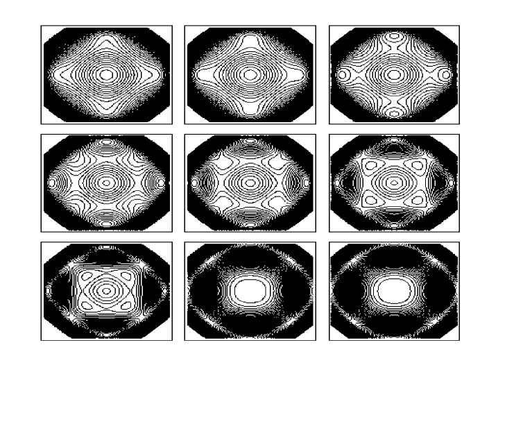
Figure 9: Contour plots of the normal form (45) illustrating the bifurcation scenario of case 1.

   A sequence of contour plots of the normal form describing this scenario is given in figure 9. The plots are arranged in order of decreasing $\zeta$. If $\zeta>0$, the central orbit is surrounded by a chain of four elliptic and four hyperbolic fixed points, representing a stable and an unstable orbit of quadruple period. At $\zeta=0$, another pair of quadruple-period orbits is created. As $\zeta$ decreases further, two subsequent tangent bifurcations occur, each of them destroying one orbit from the inner and from the outer island chain. In effect, all satellite orbits have gone, giving the overall impression as if a single period-quadrupling bifurcation had destroyed the outer island chain, whereas in fact a complicated sequence of bifurcations has taken place.

   In the remaining cases we are going to discuss, bifurcations of ghost orbits occur which cannot be seen in contour plots. Therefore, we have to resort to a different kind of presentation. In figure 10 we plot the value of the normal form $\Phi$, depending on the action coordinate $I$, for both $\sigma=+1$ and $\sigma=-1$. In these plots, a periodic orbit corresponds to a stationary point of $\Phi(I)$. If the stationary point occurs at a positive value of $I$, it indicates the presence of a real orbit, whereas a stationary point at a negative $I$ corresponds to a ghost orbit symmetric with respect to complex conjugation. Asymmetric ghost orbits correspond to stationary points at complex $I$ and are therefore invisible.

   The bifurcation scenario described above manifests itself in the plots as follows: If $\zeta>0$, there are stationary points at positive and negative values of $I$ for both $\sigma=+1$ and $\sigma=-1$. As $\zeta$ becomes negative, the stationary points at negative $I$ simultaneously cross the $\Phi$-axis and move to positive values of $I$, indicating the occurence of an island-chain-bifurcation and the appearance of two real orbits. As $\zeta$ decreases further, the two stationary points of the “$\sigma=+1$”-curve collide and disappear as the two orbits vanish in a tangent bifurcation. Subsequently, the same happens to the “$\sigma=-1$”-orbits.

2. $|a|>|b|,\quad\varrho_{\pm}>0$
   The orbits “$++$” and “$-+$” are real if $\zeta>0$. As $\zeta\searrow 0$, they simultaneously collapse onto the central periodic orbit and become ghosts, that is, at $\zeta=0$ an island-chain-bifurcation takes place. For any $\sigma$, the complex “$\sigma+$”- and “$\sigma-$”-orbits collide at $\zeta=-\varrho_{\sigma}^{2}$ and become complex conjugates. This sequence of events is depicted in figure 11.

3. $|a|<|b|,\quad\varrho_{-}<0<\varrho_{+}$
   If $\zeta>0$, the orbit “$++$” is real, whereas “$--$” is complex. As $\zeta\searrow 0$, these orbits collapse onto the central orbit and form a touch-and-go-bifurcation. In the plots of figure 12, this bifurcation manifests itself in two stationary points simultaneously crossing the $\Phi$-axis from opposite sides. At $\zeta=-\varrho_{+}^{2}$, the “$++$”-orbit, which is complex now, collides with the complex “$+-$”-orbit, and they become complex conjugate ghost orbits. Similarly, the real orbits “$--$” and “$-+$” become complex conjugates in a collision at $\zeta=-\varrho_{-}^{2}$.

4. $|a|<|b|,\quad\varrho_{+}<0<\varrho_{-}$
   This case is similar to the preceding. Following the touch-and-go-bifurcation at $\zeta=0$, the disappearences of the real and the ghost orbits now occur in reversed order (see figure 13).

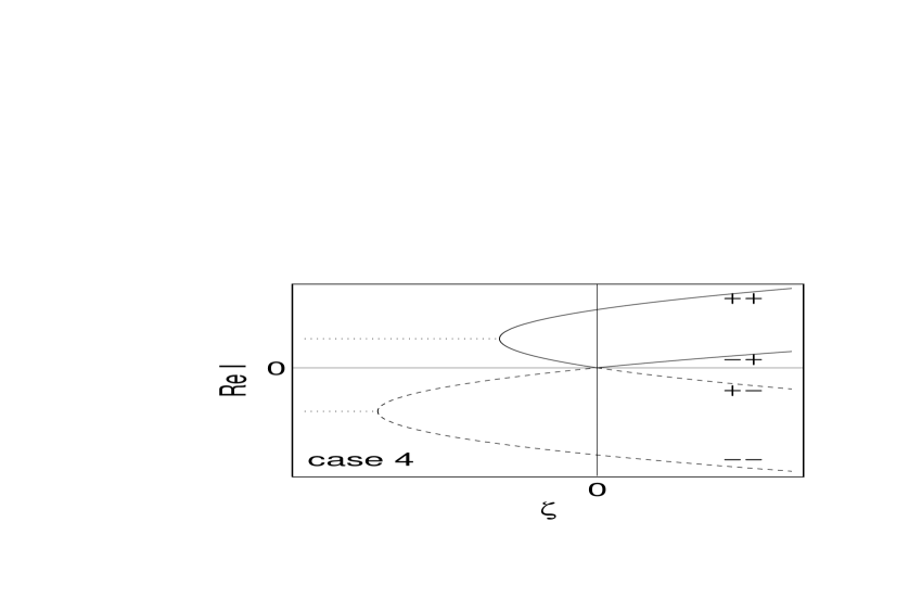
Figure 14: The four complete bifurcation scenarios the normal form (45) can describe.

Figure 14 summarizes the four bifurcation scenarios described above. As in figure 8, we plot the values of $I$ where the stationary points occur for different $\zeta$, so that the sequence of bifurcations becomes visible in a single plot.

The scenario called case 2 above is already rather similar to the situation discussed in section 3. However, in our example we observed only one of the two ghost orbit bifurcations, and there is no actual periodic orbit corresponding to the “$--$”-orbit of the normal form. To obtain a more accurate description of the bifurcation phenomenon, we adopt a slightly different normal form by setting $\lambda=\frac{d-c}{8(b-c)}$ in (44). After renaming, we obtain the modified normal form

$$\Phi=\varepsilon I+aI^{2}+bI^{2}\cos(4\varphi)+cI^{3}(1+\cos(4\varphi))\;.$$ (49)

The stationary-point equations read

$$0\stackrel{{\scriptstyle\textstyle!}}{{=}}\frac{\partial\Phi}{\partial\varphi} =-4I^{2}(b+cI)\sin(4\varphi)\;,$$ (50)

$$0\stackrel{{\scriptstyle\textstyle!}}{{=}}\frac{\partial\Phi}{\partial I} =\varepsilon+2aI+2bI\cos(4\varphi)+3cI^{2}(1+\cos(4\varphi))\;.$$

As above, it follows that

$$\sin(4\varphi)=0\;,$$

$$\cos(4\varphi)=\sigma=\pm 1\;,$$

and

$$\varepsilon+2(a+\sigma b)I+3cI^{2}(1+\sigma)=0\;.$$ (51)

If $\sigma=+1$, this agrees with equation (46) as obtained from the third-order normal form discussed above and thus yields the sequence of period quadrupling and isochronous bifurcation as found above. If $\sigma=-1$, however, the third-order term vanishes, so that there is only one further satellite orbit described by the normal form which is directly involved in the period quadrupling. To put it more precisely, the stationary points of the normal form for $\sigma=+1$ occur at

$$I_{\pm}=-\frac{a+b}{6c}\pm\sqrt{-\frac{\varepsilon}{6c}+\left(\frac{a+b}{6c}\right)^{2}}$$

and for $\sigma=-1$ at

$$I_{-1}=-\frac{\varepsilon}{2(a-b)}\;.$$

From now on, we will assume $|a|>|b|$ and $c<0$. As can be shown in a discussion similar to the above, this is the only case in which an island-chain-bifurcation occurs at $\varepsilon=0$ with the real satellites existing for positive $\varepsilon$ as we need to describe our example situation from section 3. The bifurcation scenario described by the normal form (49) in this case is shown schematically in figures 15 and 16. The sequence of an island-chain-bifurcation at $\varepsilon=0$ and a ghost orbit bifurcation at some negative value of $\varepsilon$ can easily be seen to agree with the bifurcation scenario described in section 3. Furthermore, with the help of the bifurcations the orbits undergo we can identify individual periodic orbits with stationary points of the normal form as follows: The central periodic orbit corresponds to the stationary point at $I=0$ by construction. The stationary point labelled as “$-1$” collides with the origin at $\varepsilon=0$, but does not undergo any further bifurcations. It can thus be identified with the unstable satellite orbit. Finally, the stationary points “$+$” and “$-$” agree with the stable satellite orbit and the additional ghost orbit, respectively.

Under the above assumptions, we can write

$$I_{\pm}=-c^{-1/3}\left(\delta\pm\sqrt{\eta+\delta^{2}}\right)$$ (52)

with the abbreviations

$$\begin{gathered}\eta=-\frac{\varepsilon}{6c^{1/3}}\;,\\ \delta=\frac{a+b}{6c^{2/3}}\;.\end{gathered}$$ (53)

From the decomposition

$$\Phi=\left(\frac{1}{3}I+\frac{a+b}{18c}\right)\frac{\partial\Phi}{\partial I}-4c^{1/3}\left(\eta+\delta^{2}\right)I+2\eta\delta\text{\qquad if }\cos(4\varphi)=+1\;,$$

which can be derived by a polynomial division, we then obtain the actions of periodic orbits as

$$\begin{gathered}\begin{split}\Phi_{\pm}&=\Phi(I_{\pm},\sigma=+1)\\ &=-4c^{1/3}\left(\eta+\delta^{2}\right)I_{\pm}+2\eta\delta\\ &=+4\left(\eta+\delta^{2}\right)\left(\delta\pm\sqrt{\eta+\delta^{2}}\right)+2\eta\delta\;,\end{split}\\ \Phi_{-1}=\Phi\left(I_{-1},\sigma=-1\right)=-\frac{\varepsilon^{2}}{4(a-b)}\;,\\ \Phi_{0}=\Phi(I=0)=0\;.\end{gathered}$$ (54)

Furthermore, we shall need the Hessian Determinants of the action function at the stationary points. We can calculate them in an arbitrary coordinate system in principle. However, the polar coordinate system $(I,\varphi)$ is singular at the position of the central periodic orbit, so that we cannot calculate a Hessian determinant there. Thus, we will use Cartesian coordinates. Using the transformation equations (4.1) and the relation

$$\cos(4\varphi)=\cos^{4}\varphi-6\cos^{2}\varphi\sin^{2}\varphi+\sin^{4}\varphi\;,$$

we can express the normal form in Cartesian coordinates

$$\Phi=\frac{\varepsilon}{2}(p^{2}+q^{2})+\frac{a}{4}(p^{4}+2p^{2}q^{2}+q^{4})\\ +\frac{b}{4}(p^{4}-6p^{2}q^{2}+q^{4})+\frac{c}{4}(p^{6}-p^{4}q^{2}-p^{2}q^{4}+q^{6})\;.$$ (55)

This yields the Hessian determinants

$$\begin{split}\operatorname{Hess}\Phi=&\Phi_{pp}\Phi_{qq}-\Phi_{pq}\Phi_{qp}\\ =&\left\{\varepsilon+3(a-b)p^{2}+(a-3b)q^{2}+\frac{c}{2}(15p^{4}-6p^{2}q^{2}-q^{4})\right\}\times\\ &\quad\left\{\varepsilon+(a-3b)p^{2}+3(a+b)q^{2}-\frac{c}{2}(p^{4}+6p^{2}q^{2}-15q^{4})\right\}\\ &-4p^{2}q^{2}\left\{a-3b-c(p^{2}+q^{2})\right\}^{2}\end{split}$$ (56)

If we pick $p=q=0$ on the central periodic orbit, $p=0,q=\sqrt{2I_{\pm}}$, that is, $\varphi=0$, for $\sigma=+1$, and $p=q=\frac{1}{\sqrt{2}}\sqrt{2I_{-1}}=\sqrt{I_{-1}}$, that is, $\varphi=\frac{\pi}{4}$, for $\sigma=-1$, we finally obtain Hessian determinants at the periodic orbits:

$$\begin{gathered}\operatorname{Hess}_{\pm}=\left\{\varepsilon+2(a-3b)I_{\pm}-2cI_{\pm}^{2}\right\}\left\{\varepsilon+6(a+b)I_{\pm}+30cI_{\pm}^{2}\right\}\;,\\ \operatorname{Hess}_{-1}=\left\{\varepsilon+4aI_{-1}+4cI_{-1}^{2}\right\}^{2}-4I_{-1}^{2}\left\{a-3b-2cI\right\}^{2}\;,\\ \operatorname{Hess}_{0}=\varepsilon^{2}\;.\end{gathered}$$ (57)

We have now found an analytic description of the bifurcation scenario we are discussing, and we have evaluated stationary values and Hessian determinants which we will relate to classical parameters of the orbits. We will now go over to the constuction of a uniform approximation.

5 Uniform approximation

5.1 General derivation of the uniform approximation

We need to calculate the collective contribution of all orbits involved in the bifurcation scenario to the density of states. In the derivation of the integral representation (70) of the uniform approximation, we take the method used by Sieber [35] as a guideline.

We use the semiclassical Green’s function (5) as a starting point and include the contribution of a single orbit only:

$$G({\bf x}^{\prime}{\bf x},E)=\frac{1}{i\hbar\sqrt{2\pi i\hbar}}\sqrt{|D|}\exp\left\{\frac{i}{\hbar}S({\bf x}^{\prime}{\bf x},E)-i\frac{\pi}{2}\nu\right\}\;.$$ (58)

Here, $S$ denotes the action of the periodic orbit, $\nu$ its Maslov-index, and

$$D=\det\begin{pmatrix}\frac{\partial^{2}S}{\partial{\bf x}^{\prime}\partial{\bf x}}&\frac{\partial^{2}S}{\partial{\bf x}^{\prime}\partial E}\\ [1ex]\frac{\partial^{2}S}{\partial E\partial{\bf x}}&\frac{\partial^{2}S}{\partial E^{2}}\end{pmatrix}\;.$$

As in section 4, we introduce configuration space coordinates $(y,z)$ so that $z$ is measured along the periodic orbit and increases by $2\pi$ within each circle and $y$ measures the distance form the orbit. We then have

$$\begin{split}\operatorname{Tr}G&=\int d^{2}x^{\prime}d^{2}x\,\delta({\bf x}^{\prime}-{\bf x})G({\bf x}^{\prime}{\bf x},E)\\ &=\frac{1}{i\hbar\sqrt{2\pi i\hbar}}\int d^{2}x^{\prime}d^{2}x\,\delta(z^{\prime}-z)\delta(y^{\prime}-y)\sqrt{|D|}\\ &\hskip 113.81102pt\times\exp\left\{\frac{i}{\hbar}S({\bf x}^{\prime}{\bf x},E)-i\frac{\pi}{2}\nu\right\}\\ &=\frac{1}{i\hbar m\sqrt{2\pi i\hbar}}\int dy^{\prime}dz\,dy\,\delta(y^{\prime}-y)\sqrt{|D|}\\ &\hskip 113.81102pt\times\exp\left\{\frac{i}{\hbar}S({\bf x}^{\prime}{\bf x},E)-i\frac{\pi}{2}\nu\right\}\Bigg{|}_{z^{\prime}=z+2\pi m}\;.\end{split}$$

In the last step, the $z^{\prime}$-integration has been performed. Close to an $\frac{n}{m}$-resonance, we regard $m$ periods of the bifurcating orbit as the central periodic orbit, so that the $z$-integration extends over $m$ primitive periods, although it should only extend over one. This error is corrected by the prefactor $\frac{1}{m}$.

From its definition (6), the action integral $S({\bf x}^{\prime}{\bf x},E)$ obviously satisfies

$$\frac{\partial S}{\partial{\bf x}^{\prime}}={\bf p}^{\prime}\;,\qquad\qquad\frac{\partial S}{\partial{\bf x}}=-{\bf p}\;.$$ (59)

We can thus regard $S$ as the coordinate representation of the generating function of the $m$-traversal Poincaré map. At a resonance, however, the Poincaré map is approximately equal to the identity map whose generating function does not possess a representation depending on old and new coordinates. Thus, we go over to a coordinate-momentum-representation. To this end, we substitute the integral representation

$$\delta(y^{\prime}-y)=\frac{1}{2\pi\hbar}\int_{-\infty}^{+\infty}dp_{y}^{\prime}\,\exp\left\{\frac{i}{\hbar}p^{\prime}_{y}(y-y^{\prime})\right\}$$

into (5.1) and evaluate the $y^{\prime}$-integration using the stationary-phase approximation. The stationarity condition reads

$$\frac{\partial S}{\partial y^{\prime}}-p_{y}^{\prime}=0\;,$$ (60)

so that we obtain

$$\operatorname{Tr}G=\frac{1}{2\pi im\hbar^{2}}\int dy\,dz\,dp_{y}^{\prime}\sqrt{|D|\big{|}_{\text{sp}}}\\ \times\exp\left\{\frac{i}{\hbar}\left(\hat{S}+yp_{y}^{\prime}\right)-i\frac{\pi}{2}\hat{\nu}\right\}\frac{1}{\sqrt{\left.\left|\frac{\partial^{2}S}{\partial y^{\prime}{}^{2}}\right|\right|_{\text{sp}}}}\;.$$ (61)

Here,

$$\hat{S}(z^{\prime}p_{y}^{\prime}zy,E)=S(z^{\prime}y^{\prime}z\,y,E)-y^{\prime}p_{y}^{\prime}\big{|}_{\text{sp}}$$ (62)

denotes the Legendre-transform of $S$ with respect to $y^{\prime}$ due to (60), and

$$\hat{\nu}=\begin{cases}\nu&:\left.\frac{\partial^{2}S}{\partial y^{\prime}{}^{2}}\right|_{\text{sp}}>0\\[3.44444pt] \nu+1&:\left.\frac{\partial^{2}S}{\partial y^{\prime}{}^{2}}\right|_{\text{sp}}<0\end{cases}\;.$$ (63)

As a general property of Legendre transforms, if we let $u,v$ denote any of the variables $z,z^{\prime},y,$ and $E$ which are not involved in the transformation, we have

$$\frac{\partial\hat{S}}{\partial u}=\frac{\partial S}{\partial u}\;,\hskip 56.9055pt\frac{\partial\hat{S}}{\partial p_{y}^{\prime}}=-y^{\prime}\;.$$ (64)

For the second derivatives, it follows that

$$\frac{\partial^{2}S}{\partial u\partial v} =\frac{\partial}{\partial u}\frac{\partial\hat{S}}{\partial v}$$

$$=\frac{\partial^{2}\hat{S}}{\partial u\partial v}+\frac{\partial^{2}\hat{S}}{\partial p_{y}^{\prime}\partial v}\frac{\partial p_{y}^{\prime}}{\partial u}\Big{|}_{y^{\prime}}$$ (65)

and

$$\frac{\partial^{2}S}{\partial u\partial y^{\prime}} =\frac{\partial p_{y}^{\prime}}{\partial u}$$

$$=\frac{\partial}{\partial y^{\prime}}\frac{\partial\hat{S}}{\partial u}$$

$$=\frac{\partial^{2}\hat{S}}{\partial p_{y}^{\prime}\partial u}\frac{\partial p_{y}^{\prime}}{\partial y^{\prime}}=\frac{\partial^{2}\hat{S}}{\partial p_{y}^{\prime}\partial u}\frac{\partial^{2}S}{\partial y^{\prime}{}^{2}}\;.$$ (66)

Furthermore, we have

$$D =\det\begin{pmatrix}\frac{\partial^{2}S}{\partial z^{\prime}\partial z}&\frac{\partial^{2}S}{\partial y^{\prime}\partial z}&\frac{\partial^{2}S}{\partial E\partial z}\\[4.30554pt] \frac{\partial^{2}S}{\partial z^{\prime}\partial y}&\frac{\partial^{2}S}{\partial y^{\prime}\partial y}&\frac{\partial^{2}S}{\partial E\partial y}\\[4.30554pt] \frac{\partial^{2}S}{\partial z^{\prime}\partial E}&\frac{\partial^{2}S}{\partial y^{\prime}\partial E}&\frac{\partial^{2}S}{\partial E^{2}}\end{pmatrix}$$

$$=\det\begin{pmatrix}\frac{\partial^{2}\hat{S}}{\partial z^{\prime}\partial z}+\frac{\partial^{2}\hat{S}}{\partial p_{y}^{\prime}\partial z^{\prime}}\frac{\partial p_{y}^{\prime}}{\partial z}&\frac{\partial p_{y}^{\prime}}{\partial z}&\frac{\partial^{2}\hat{S}}{\partial E\partial z}+\frac{\partial^{2}\hat{S}}{\partial p_{y}^{\prime}\partial E}\frac{\partial p_{y}^{\prime}}{\partial z}\\[4.30554pt] \frac{\partial^{2}\hat{S}}{\partial z^{\prime}\partial y}+\frac{\partial^{2}\hat{S}}{\partial p_{y}^{\prime}\partial z^{\prime}}\frac{\partial p_{y}^{\prime}}{\partial y}&\frac{\partial p_{y}^{\prime}}{\partial y}&\frac{\partial^{2}\hat{S}}{\partial E\partial y}+\frac{\partial^{2}\hat{S}}{\partial p_{y}^{\prime}\partial E}\frac{\partial p_{y}^{\prime}}{\partial y}\\[4.30554pt] \frac{\partial^{2}\hat{S}}{\partial z^{\prime}\partial E}+\frac{\partial^{2}\hat{S}}{\partial p_{y}^{\prime}\partial z^{\prime}}\frac{\partial p_{y}^{\prime}}{\partial E}&\frac{\partial p_{y}^{\prime}}{\partial E}&\frac{\partial^{2}\hat{S}}{\partial E^{2}}+\frac{\partial^{2}\hat{S}}{\partial p_{y}^{\prime}\partial E}\frac{\partial p_{y}^{\prime}}{\partial E}\end{pmatrix}\;.$$

The second terms in the first and third columns of this matrix are multiples of the second column, and can thus be omitted. This yields

$$\begin{split}D&=\det\begin{pmatrix}\frac{\partial^{2}\hat{S}}{\partial z^{\prime}\partial z}&\frac{\partial^{2}S}{\partial y^{\prime}{}^{2}}\frac{\partial^{2}\hat{S}}{\partial p_{y}^{\prime}\partial z}&\frac{\partial^{2}\hat{S}}{\partial E\partial z}\\[4.30554pt] \frac{\partial^{2}\hat{S}}{\partial z^{\prime}\partial y}&\frac{\partial^{2}S}{\partial y^{\prime}{}^{2}}\frac{\partial^{2}\hat{S}}{\partial p_{y}^{\prime}\partial y}&\frac{\partial^{2}\hat{S}}{\partial E\partial y}\\[4.30554pt] \frac{\partial^{2}\hat{S}}{\partial z^{\prime}\partial E}&\frac{\partial^{2}S}{\partial y^{\prime}{}^{2}}\frac{\partial^{2}\hat{S}}{\partial p_{y}^{\prime}\partial E}&\frac{\partial^{2}\hat{S}}{\partial E^{2}}\end{pmatrix}\\ &=\frac{\partial^{2}S}{\partial y^{\prime}{}^{2}}\,\det\begin{pmatrix}\frac{\partial^{2}\hat{S}}{\partial z^{\prime}\partial z}&\frac{\partial^{2}\hat{S}}{\partial p_{y}^{\prime}\partial z}&\frac{\partial^{2}\hat{S}}{\partial E\partial z}\\[4.30554pt] \frac{\partial^{2}\hat{S}}{\partial z^{\prime}\partial y}&\frac{\partial^{2}\hat{S}}{\partial p_{y}^{\prime}\partial y}&\frac{\partial^{2}\hat{S}}{\partial E\partial y}\\[4.30554pt] \frac{\partial^{2}\hat{S}}{\partial z^{\prime}\partial E}&\frac{\partial^{2}\hat{S}}{\partial p_{y}^{\prime}\partial E}&\frac{\partial^{2}\hat{S}}{\partial E^{2}}\end{pmatrix}\;.\end{split}$$ (67)

If we denote the remaining determinant by $\hat{D}$, we obtain from (61)

$$\operatorname{Tr}G=\frac{1}{2\pi im\hbar^{2}}\int dy\,dz\,dp_{y}^{\prime}\sqrt{|\hat{D}|}\,\exp\left\{\frac{i}{\hbar}\left(\hat{S}+yp_{y}^{\prime}\right)-i\frac{\pi}{2}\hat{\nu}\right\}\Bigg{|}_{z^{\prime}=z+2\pi m}\;.$$

From our choice of $z$ along the periodic orbit, we have

$$\frac{\partial H}{\partial{\bf p}}=\dot{{\bf x}}=(\dot{z},0)\;.$$

Taking derivatives of the Hamilton-Jacobi equations

$$H\left(\frac{\partial S}{\partial{\bf x}^{\prime}},{\bf x}^{\prime}\right)=E\;,\qquad\qquad H\left(-\frac{\partial S}{\partial{\bf x}},{\bf x}\right)=E$$

with respect to $z,z^{\prime}$ and $y$ and using (64), we therefore obtain

$$\frac{\partial^{2}\hat{S}}{\partial z^{\prime}\partial z}=\frac{\partial^{2}\hat{S}}{\partial p_{y}^{\prime}\partial z}=\frac{\partial^{2}\hat{S}}{\partial z^{\prime}\partial y}=0\;,$$

$$\frac{\partial^{2}\hat{S}}{\partial z^{\prime}\partial E}=\frac{1}{\dot{z}^{\prime}}\;,\qquad\qquad\frac{\partial^{2}\hat{S}}{\partial E\partial z}=\frac{1}{\dot{z}}\;,$$

so that

$$\hat{D}=\frac{1}{\dot{z}\dot{z}^{\prime}}\frac{\partial^{2}\hat{S}}{\partial y\partial p_{y}^{\prime}}\;.$$ (68)

Using this relation, the $z$-integration can trivially be performed. It yields the time consumed during one cycle. This time depends on the coordinates $y$ and $p_{y}$ and is different in general from the orbital period of the central periodic orbit. We denote it by $\frac{\partial\hat{S}}{\partial E}(y,p_{y}^{\prime})$:

$$\operatorname{Tr}G=\frac{1}{2\pi im\hbar^{2}}\int dy\,dp_{y}^{\prime}\frac{\partial\hat{S}}{\partial E}\sqrt{\left|\frac{\partial^{2}\hat{S}}{\partial y\partial p_{y}^{\prime}}\right|}\,\exp\left\{\frac{i}{\hbar}\left(\hat{S}+yp_{y}^{\prime}\right)-i\frac{\pi}{2}\hat{\nu}\right\}\;.$$ (69)

Finally, we obtain the contribution of the orbits under study to the density of states:

$$\begin{split}d(E)&=-\frac{1}{\pi}\,{\rm Im}\,\operatorname{Tr}G\\ &=\frac{1}{2\pi^{2}m\hbar^{2}}\,{\rm Re}\,\int dy\,dp_{y}^{\prime}\frac{\partial\hat{S}}{\partial E}\sqrt{\left|\frac{\partial^{2}\hat{S}}{\partial y\partial p_{y}^{\prime}}\right|}\\ &\hskip 113.81102pt\times\exp\left\{\frac{i}{\hbar}\left(\hat{S}+yp_{y}^{\prime}\right)-i\frac{\pi}{2}\hat{\nu}\right\}\;.\end{split}$$ (70)

The exponent function

$$f(y,p_{y}^{\prime},E):=\hat{S}(y,p_{y}^{\prime},E)+yp_{y}^{\prime}$$ (71)

has to be related to known functions. The only information on $f$ we possess is the distribution of its stationary points: They correspond to classical periodic orbits.

The classification of real-valued functions with respect to the distribution of their stationary points is achieved within the mathematical framework of catastrophe theory [27]. The object of study there are families of functions $\Phi({\bf x},Z)$ depending on $k$ so-called state variables ${\bf x}$ and indexed by $r$ control variables $Z$. For any fixed control $Z$, the function $\Phi({\bf x},Z)$ is assumed to have a stationary point at the origin and to take 0 as its stationary value there. Further stationary points may or may not exist in a neighborhood of the origin. As the control parameters are varied, such additional stationary points may collide with the central stationary point, they may be born or destroyed. The aim of catastrophe theory is to qualitatively understand how these bifurcations of stationary points can take place. More precisely, two families $\Phi_{1}$ and $\Phi_{2}$ of functions as described above are regarded as eqivalent if there is a diffeomorphism $\psi_{c}$ of control space and a control-dependent family $\psi_{s}(Z)$ of diffeomorphisms of state space which keep the origin fixed, such that

$$\Phi_{2}({\bf x},Z)=\Phi_{1}(\psi_{s}({\bf x},Z),\psi_{c}(Z))\;.$$ (72)

Equivalence classes with respect to this relation are known as catastrophes. Catastrophes having a codimension of at most four, that is, catastrophes which can generically be observed if no more than four control parameters are varied, have completely been classified by Thom. They are known as the seven elementary catastrophes. Each of these catastrophes can be represented by a polynomial in one or two variables.

In our discussion of periodic orbits the energy serves as the only control parameter. However, we are only interested in stationary points of functions which can be obtained as action functions in Hamiltonian systems. Due to this restriction, we can generically observe scenarios which would have higher codimensions in the general context of catastrophe theory, so that catastrophes of codimension greater than one are relevant for our purpose. The variation of energy then defines a path $Z(E)$ in an abstract higher-dimensional control space.

In earlier work on the contruction of uniform approximations close to nongeneric bifurcations, Main and Wunner [20, 21] succeeded in relating the action function describing the bifurcation scenario to one of the elementary catastrophes. In our case, however, this approach fails because the codimension (in the sense of catastrophe theory) of the action function is even higher than four. Nevertheless, we can make use of the equivalence relation of catastrophe theory, because, as was shown above, the normal form has got stationary points which exactly correspond to the periodic orbits of the classical system. This observation enables us in principle to systematically construct ansatz functions for any bifurcation scenario encountered in a Hamiltonian system using normal form theory. We are thus led to making the ansatz

$$f(y,p_{y}^{\prime};E)=S_{0}(E)+\Phi(\psi_{s}(y,p_{y}^{\prime};E),\psi_{c}(E))\;.$$ (73)

Here, the energy $E$ serves as the control parameter, $\Phi$ denotes the normal form of the bifurcation scenario, $\psi_{s}$ and $\psi_{c}$ unknown coordinate changes as in the general context of catastrophe theory, and $S_{0}(E)$ is the action of the central periodic orbit, which has to be introduced here to make both sides equal at the origin. The unknown transformations $\psi_{s}$ and $\psi_{c}$ can easily be accounted for because they can only manifest themselves in appropriate choices of the free parameters occuring in the normal form. Inserting the ansatz (73) into (70) and transforming the integration measure to new coordinates $(Y,P_{Y}^{\prime})=\psi_{s}(y,p_{y}^{\prime};E)$, we obtain

$$d(E)=\frac{1}{2\pi^{2}m\hbar^{2}}\,{\rm Re}\,\exp\left\{\frac{i}{\hbar}S_{0}(E)-i\frac{\pi}{2}\hat{\nu}\right\}\\ \times\int dYdP_{Y}^{\prime}\frac{\partial\hat{S}}{\partial E}\sqrt{\left|\frac{\partial^{2}\hat{S}}{\partial y\partial p_{y}^{\prime}}\right|}\frac{1}{|\det\operatorname{Jac}\psi_{s}|}\exp\left\{\frac{i}{\hbar}\Phi(Y,P_{Y}^{\prime})\right\}\;,$$

where $\operatorname{Jac}\psi_{s}$ denotes the Jacobian matrix of $\psi_{s}$ with respect to the variables $y$ and $p_{y}^{\prime}$. Differentiating the ansatz (73) twice, we get the matrix equation

$$\frac{\partial^{2}f}{\partial(y,p_{y}^{\prime})^{2}}=(\operatorname{Jac}\psi_{s})^{T}\frac{\partial^{2}\Phi}{\partial(Y,P_{Y}^{\prime})^{2}}\operatorname{Jac}\psi_{s}\;,$$

so that the determinants satisfy

$$|\det\operatorname{Jac}\psi_{s}|=\sqrt{\frac{|\operatorname{Hess}f|}{|\operatorname{Hess}\Phi|}}\;,$$ (74)

and the density of states finally reads

$$d(E)=\frac{1}{2\pi^{2}m\hbar^{2}}\,{\rm Re}\,\exp\left\{\frac{i}{\hbar}S_{0}(E)-i\frac{\pi}{2}\hat{\nu}\right\}\\ \times\int dYdP_{Y}^{\prime}\frac{\partial\hat{S}}{\partial E}\sqrt{\left|\frac{\partial^{2}\hat{S}}{\partial y\partial p_{y}^{\prime}}\right|}\sqrt{\frac{|\operatorname{Hess}\Phi|}{|\operatorname{Hess}f|}}\exp\left\{\frac{i}{\hbar}\Phi(Y,P_{Y}^{\prime})\right\}\;.$$ (75)

The exponent function in the integrand of the remaining integral is given by the normal form describing the bifurcation scenario, which was calculated in the preceding section for the present case. The normal form parameters, however, still have to be determined. On the other hand, the coefficient

$$X:=\frac{\partial\hat{S}}{\partial E}\sqrt{\left|\frac{\partial^{2}\hat{S}}{\partial y\partial p_{y}^{\prime}}\right|}\sqrt{\frac{|\operatorname{Hess}\Phi|}{|\operatorname{Hess}f|}}$$ (76)

is completely unknown. To evaluate (75), we have to establish a connection between $X$ and classical periodic orbits. As periodic orbits correspond to stationary points of the normal form, we will now analyse the behavior of $X$ at stationary points of the exponent.

By (71), the Hessian matrix of $f$ is given by

$$\frac{\partial^{2}f}{\partial(y,p_{y}^{\prime})^{2}}=\begin{pmatrix}\frac{\partial^{2}\hat{S}}{\partial y^{2}}&\frac{\partial^{2}\hat{S}}{\partial y\partial p_{y}^{\prime}}+1\\[4.30554pt] \frac{\partial^{2}\hat{S}}{\partial y\partial p_{y}^{\prime}}+1&\frac{\partial^{2}\hat{S}}{\partial p_{y}^{\prime}{}^{2}}\end{pmatrix}$$

so that the Hessian determinant reads

$$\begin{split}\operatorname{Hess}f&=\frac{\partial^{2}\hat{S}}{\partial y^{2}}\frac{\partial^{2}\hat{S}}{\partial p_{y}^{\prime}{}^{2}}-\left(\frac{\partial^{2}\hat{S}}{\partial y\partial p_{y}^{\prime}}+1\right)^{2}\\ &=-\left(1+\left(\frac{\partial^{2}\hat{S}}{\partial y\partial p_{y}^{\prime}}\right)^{2}-\frac{\partial^{2}\hat{S}}{\partial y^{2}}\frac{\partial^{2}\hat{S}}{\partial p_{y}^{\prime}{}^{2}}\right)-2\frac{\partial^{2}\hat{S}}{\partial y\partial p_{y}^{\prime}}\;.\end{split}$$

As can be shown, in a two-degree-of-freedom system the monodromy matrix of a periodic orbit can be expressed in terms of the action function as

$$\operatorname{Tr}M=-\left(\frac{\partial^{2}\hat{S}}{\partial y\partial p_{y}^{\prime}{}}\right)^{-1}\left\{1+\left(\frac{\partial^{2}\hat{S}}{\partial y\partial p_{y}^{\prime}{}}\right)^{2}-\frac{\partial^{2}\hat{S}}{\partial y^{2}}\frac{\partial^{2}\hat{S}}{\partial p_{y}^{\prime}{}^{2}}\right\}\;,$$ (77)

so that

$$\operatorname{Hess}f\stackrel{{\scriptstyle\text{sp}}}{{=}}(\operatorname{Tr}M-2)\frac{\partial^{2}\hat{S}}{\partial y\partial p_{y}^{\prime}}$$ (78)

and

$$\sqrt{\frac{1}{|\operatorname{Hess}f|}}\sqrt{\left|\frac{\partial^{2}\hat{S}}{\partial y\partial p_{y}^{\prime}}\right|}\stackrel{{\scriptstyle\text{sp}}}{{=}}\frac{1}{\sqrt{|\operatorname{Tr}M-2|}}\;.$$ (79)

Furthermore, we make use of the fact that at a stationary point the derivative $\partial\hat{S}/\partial E$ gives the orbital period of the corresponding periodic orbit. For the central periodic orbit, this is $m$ times the primitive period $mT_{0}$, for a satellite orbit, however, it gives a single primitive period $T_{s}$. Altogether, these results yield

$$X\stackrel{{\scriptstyle\text{sp}}}{{=}}\frac{\{m\}T}{\sqrt{|\operatorname{Tr}M-2|}}\sqrt{|\operatorname{Hess}\Phi|}\;,$$ (80)

where the notation $\{m\}$ is meant to indicate that the factor of $m$ has to be omitted for a satellite orbit. This expression can be calculated once the normal form parameters have suitably been determined.

Furthermore, (80) allows us to check that (75) does indeed reduce to Gutzwiller’s isolated-orbits contributions if the distance from the bifurcations is large: If the stationary points of the normal form are sufficiently isolated, we can return to a stationary-phase approximation of the integral. We will first calculate the contribution of the stationary point at $Y=P_{Y}^{\prime}=0$, which corresponds to the central periodic orbit. If we use $\Phi(0)=0$ and (80) and let $\lambda$ denote the number of negative eigenvalues of the Hessian matrix $\left.\frac{\partial^{2}\Phi}{\partial(Y^{\prime},P_{Y})^{2}}\right|_{0}$, this contribution reads

$$\begin{split}&\quad\frac{1}{2\pi^{2}m\hbar^{2}}\frac{mT_{0}}{\sqrt{\operatorname{Tr}M_{0}-2}}\sqrt{|\operatorname{Hess}\Phi|\big{|}_{0}}\,{\rm Re}\,\exp\left\{\frac{i}{\hbar}S_{0}-i\frac{\pi}{2}\hat{\nu}\right\}\,(2\pi i\hbar)\frac{\exp\left\{-i\frac{\pi}{2}\lambda\right\}}{\sqrt{|\operatorname{Hess}\Phi|\big{|}_{0}}}\\ &=\frac{1}{\pi\hbar}\frac{T_{0}}{\sqrt{\operatorname{Tr}M_{0}-2}}\,{\rm Re}\,\exp\left\{\frac{i}{\hbar}S_{0}-i\frac{\pi}{2}\left(\hat{\nu}+\lambda-1\right)\right\}\;.\end{split}$$

If we identify $\hat{\nu}+\lambda-1$ with the Maslov index of the central periodic orbit, and note that in a two-degree-of-freedom system $\operatorname{Tr}M-2=\det(M-I)$, this is just Gutzwiller’s periodic-orbit contribution.

Satellite orbits contribute only at energies where they are real. In this case, every satellite orbit corresponds to $m$ stationary points of the normal form. Altogether, they contribute

$$\begin{split}&\quad m\frac{1}{2\pi^{2}m\hbar^{2}}\frac{T_{s}}{4\sqrt{\operatorname{Tr}M_{s}-2}}\sqrt{|\operatorname{Hess}\Phi|\big{|}_{s}}\\ &\qquad\qquad{\rm Re}\,\exp\left\{\frac{i}{\hbar}S_{0}-i\frac{\pi}{2}\hat{\nu}\right\}\,(2\pi i\hbar)\exp\left\{\frac{i}{\hbar}\Phi_{s}\right\}\frac{\exp\left\{-i\frac{\pi}{2}\lambda^{\prime}\right\}}{\sqrt{|\operatorname{Hess}\Phi|\big{|}_{s}}}\\ &=\frac{1}{\pi\hbar}\frac{T_{s}}{\sqrt{\operatorname{Tr}M_{s}-2}}{\rm Re}\,\exp\left\{\frac{i}{\hbar}S_{s}-i\frac{\pi}{2}\left(\hat{\nu}+\lambda^{\prime}-1\right)\right\}\;.\end{split}$$

Here, the number of negative eigenvalues of $\left.\frac{\partial^{2}\Phi}{\partial(Y^{\prime},P_{Y})^{2}}\right|_{s}$ was denoted by $\lambda^{\prime}$, and we made use of the fact that, according to our ansatz (73), $S_{0}(E)+\Phi_{s}$ equals the action $S_{s}(E)$ of the satellite orbit. Thus, we also obtain Gutzwiller’s contribution for satellite orbits, provided that $\hat{\nu}+\lambda^{\prime}-1$ is the Maslov index of the satellite orbit. We can regard this as a consistency condition which allows us to calculate the difference in Maslov index between the central periodic orbit and the satellites from the normal form.

Now that we have convinced ourselves that the integral formula (75) is correct, we can go over to its numerical evaluation. This can be done to different degrees of approximation, and we are going to present two different approximations in the following sections.

5.2 Local Approximation

To obtain the simplest approximation possible, we can try to determine the normal form parameters $a,b,c$ so that the stationary values (54) of the normal form (49) globally reproduce the actions of the periodic orbits as well as possible. In the spirit of the stationary-phase method we can further assume the integral in (75) to be dominated by those parts of the coordinate plane where the stationary points of the exponent are located. As the uniform approximation is only needed close to a bifurcation, where the stationary-phase approximation fails, all stationary points lie in a neighborhood of the origin $I=0$. Thus, we can approximate the derivative $\partial\hat{S}/\partial E$ by its value at the origin, that is, the orbital period $mT_{0}$ of the central periodic orbit. Furthermore, we can try and approximate the quotient $(\operatorname{Tr}M-2)/\operatorname{Hess}\Phi$ by a constant $k$. We then obtain

$$d(E)\approx\frac{1}{2\pi^{2}\hbar^{2}}\frac{T_{0}}{\sqrt{|k|}}\,{\rm Re}\,\exp\left\{\frac{i}{\hbar}S_{0}(E)-i\frac{\pi}{2}\hat{\nu}\right\}\\ \times\int dYdP_{Y}^{\prime}\exp\left\{\frac{i}{\hbar}\Phi(Y,P_{Y}^{\prime})\right\}\;.$$ (81)

Thus, the density of states is approximately given by the integral of a known function which can be evaluated numerically.

In our case, the distance from the period-quadrupling bifurcation is described by the normal form parameter $\varepsilon$. We choose to measure this distance by the difference in scaled energy

$$\varepsilon=\tilde{E}-\tilde{E}_{c}\;.$$ (82)

Then, to globally reproduce the numerically calculated actions, we use the parameter values

$$\tilde{a} =-0.029\;,$$ (83)

$$\tilde{b} =+0.007\;,$$

$$\tilde{c} =-0.052\;,$$

$$\tilde{k} =11000\;,$$

where the tilde indicates that the parameters have been adjusted to the scaled actions $\tilde{S}/2\pi$. As can be seen from figures 17 and 18, the action differences and Hessian determinants calculated from the normal form do indeed qualitatively reproduce the acual data, although quantitatively the agreement is not very good. Nevertheless, we will try and calculate the density of states within the present approximation.

If we are actually going to calculate spectra for different values of the magnetic field strength, we have to determine the action $S=2\pi w\cdot(\tilde{S}/2\pi)$ according to the scaling prescription (10) with the scaling parameter $w=\gamma^{-1/3}$. As can easily be seen with the help of (54), this scaling can be achieved by scaling the normal form parameters according to

$$a =\tilde{a}/2\pi w\;,$$ (84)

$$b =\tilde{b}/2\pi w\;,$$

$$c =\tilde{c}/4\pi^{2}w^{2}\;.$$

According to its definition (82), the parameter $\varepsilon$ does not scale. Neither does $k$ scale with the magnetic field strength, because it is given by a quotient of two non-scaling quantities, but the factor of $2\pi$ in $\operatorname{Hess}\Phi$ has to be taken into account:

$$k=\tilde{k}/2\pi\;.$$ (85)

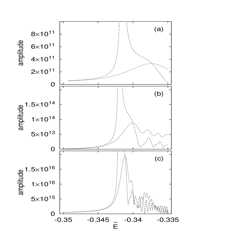
Figure 19: Local approximation to the contribution of the considered bifurcation scenario to the density of states for three different values of the magnetic field strength: (a) $\gamma=10^{-10}$, (b) $\gamma=10^{-12}$, (c) $\gamma=10^{-14}$. Solid curves: local approximation, dashed curves: Gutzwiller’s trace formula.

The local approximation calculated with these data is shown in figure 19 for three different values of the magnetic field strength. Instead of the real part, we actually plotted the absolute value of the expression in (81) to suppress the highly oscillatory factor $\exp\left\{\frac{i}{\hbar}S_{0}(E)\right\}$. As was to be expected, the approximation does indeed give finite values at the bifurcation points, but does not reproduce the results of Gutzwiller’s trace formula as the distance from the bifurcations is increased. This is due to the fact that the normal form with the parameter values chosen does not reproduce the actual orbital data very well. In particular, a better description of the actions is needed to improve the approximation, because asymptotically the actions occur as phases in Gutzwiller’s trace formula, so that, if the error in phases $w\tilde{S}$ is not small compared to $2\pi$, the interference effects between the contributions of different orbits cannot correctly be described.

Furthermore, we cannot even expect our local approximation to yield very accurate values at the bifurcation points themselves, because the normal form parameters were chosen to globally reproduce the orbital data, so that a local parameter fit designed to describe the immediate neighborhood of the bifurcations would lead to different results.

5.3 Uniform Approximation

To improve our approximation, we can make use of the fact that the coordinate transformation $\psi_{s}$ in (73) is energy-dependent in general, so that the normal form parameters $a,b,c$ will also depend on energy. We thus have to choose the parameters so as to reproduce the numerically calculated action differences for any fixed $\varepsilon=\tilde{E}-\tilde{E}_{c}$. To achieve this, we have to solve equations (54)

$$\begin{gathered}\Phi_{\pm}=4(\eta+\delta^{2})\left(\delta\pm\sqrt{\eta+\delta^{2}}\right)+2\eta\delta\;,\\ \Phi_{-1}=-\frac{\varepsilon^{2}}{4(a-b)}\;,\end{gathered}$$ (86)

where

$$\begin{gathered}\eta=-\frac{\varepsilon}{6c^{1/3}}\;,\\ \delta=\frac{a+b}{6c^{2/3}}\;,\end{gathered}$$ (87)

for $a,b,c$. To this end, we introduce

$$\begin{split}h_{+}&=\frac{\Phi_{+}+\Phi_{-}}{8}\\ &=\delta\left(\eta+\delta^{2}\right)+\frac{1}{2}\eta\delta\;,\\ h_{-}&=\frac{\Phi_{+}-\Phi_{-}}{8}\\ &=(\eta+\delta^{2})^{3/2}\;.\end{split}$$ (88)

The second equation yields

$$\eta=h_{-}^{2/3}-\delta^{2}\;.$$ (89)

Inserting this into the first equation of (88), we obtain

$$\delta^{3}-3h_{-}^{2/3}\delta+2h_{+}=0\;.$$ (90)

This is a cubic equation for $\delta$. Its solutions read, from Cardani’s formula,

$$\delta=\frac{\lambda}{2}\sqrt[3]{-\left(\sqrt{\Phi_{+}}+\sqrt{\Phi_{-}}\right)^{2}}+\frac{\lambda^{\ast}}{2}\sqrt[3]{-\left(\sqrt{\Phi_{+}}-\sqrt{\Phi_{-}}\right)^{2}}\;,$$ (91)

where $\lambda\in\{1,-\frac{1}{2}\pm i\frac{\sqrt{3}}{2}\}$ is a cube root of unity. If the discriminant

$$D=h_{+}^{2}-h_{-}^{2}=\frac{1}{16}\Phi_{+}\Phi_{-}\;,$$ (92)

is positive, there is only one real solution for $\delta$, which has $\lambda=1$. If, however, $D<0$, all three solutions are real. In this case we have to choose one solution before we can proceed.

Using the correspondence between stationary points and periodic orbits discussed above, we find from figure 6 that $\Phi_{+}>0$, and there exists an $\varepsilon_{0}<0$ so that $\Phi_{-}<0$ if $\varepsilon>\varepsilon_{0}$ and $\Phi_{-}>0$ if $\varepsilon<\varepsilon_{0}$. Thus, from (92), we have $D\lessgtr 0$ if $\varepsilon\gtrless\varepsilon_{0}$, and we have to choose $\lambda=1$ if $\varepsilon<\varepsilon_{0}$ to make $\delta$ real.

To determine the correct choice of $\lambda$ for $\varepsilon>\varepsilon_{0}$, we demand that $\delta$ must depend on $\varepsilon$ continuously. Thus, $\lambda$ can only change at energies where (90) has a double root, viz.  $D=0$ or $\varepsilon\in\{0,\varepsilon_{0}\}$. Therefore, it suffices to determine $\lambda$ in a neighborhood of $\varepsilon=0$. Close to $\varepsilon=0$, the action differences can be seen from figure 6 to behave like

$$\Phi_{+} =\alpha^{2}\varepsilon^{2}+{\cal O}\left(\varepsilon^{3}\right)\;,$$

$$\Phi_{-} =-\Gamma-\beta\varepsilon+{\cal O}\left(\varepsilon^{2}\right)$$

with positive real constants $\alpha,\beta,\Gamma$. Equations (91) and (89) then allow us to expand $\eta$ in a Taylor series in $\varepsilon$:

$$\eta=\left(\frac{1}{4}-({\rm Re}\,\lambda)^{2}\right)\Gamma^{2/3}\\ +\left(\left(\frac{1}{4}-({\rm Re}\,\lambda)^{2}\right)\frac{2\beta}{3\Gamma^{1/3}}-{\rm Re}\,\lambda\,{\rm Im}\,\lambda\,\frac{4\alpha\operatorname{sign}\varepsilon\sqrt{\Gamma}}{3\Gamma^{1/3}}\right)\varepsilon+{\cal O}\left(\varepsilon^{2}\right)$$ (93)

If we require this result to reproduce the definition

$$\eta=-\frac{1}{6c^{1/3}}\varepsilon,\qquad\qquad-\frac{1}{6c^{1/3}}>0\;,$$

we find the conditions

$${\rm Re}\,\lambda=-\frac{1}{2}\;,$$

$${\rm Im}\,\lambda\,\frac{2\alpha\sigma}{3\Gamma^{1/3}}>0\;;$$

and are thus led to the correct choices of $\lambda$:

$$\lambda=\begin{cases}1&:\Phi_{-}>0\\ -\frac{1}{2}+i\frac{\sqrt{3}}{2}\operatorname{sign}\varepsilon&:\Phi_{-}<0\end{cases}\;.$$ (94)

Using this result, we obtain $\delta$ and $\eta$ from (91) and (89). Finally, from (53) and (86) we can explicitly determine the normal form parameters $a,b,c$ as functions of the energy $\varepsilon$ and the action differences $\Phi_{+},\Phi_{-},$ and $\Phi_{-1}$:

$$\begin{gathered}c=-\left(\frac{\varepsilon}{6\eta}\right)^{3}\;,\\ a+b=6c^{2/3}\delta\;,\qquad\qquad a-b=-\frac{\varepsilon}{4\Phi_{-1}}\;,\\ a=3c^{2/3}\delta-\frac{\varepsilon}{8\Phi_{-1}}\;,\qquad\qquad b=3c^{2/3}\delta+\frac{\varepsilon}{8\Phi_{-1}}\;.\end{gathered}$$ (95)

Now that the normal form $\Phi$ has been completely specified, a suitable approximation to the coefficient $X$ remains to be found. We shall assume $X$ to be independent of the angular coordinate $\varphi$, and because, from (80), the value of $X$ is known at the stationary points of $f$ at four different values of $I$ (including $I=0$), we can approximate $X$ by the third-order polynomial $p(I)$ interpolating between the four given points, so that our uniform approximation takes its final form

$$d(E)=\frac{1}{2\pi^{2}m\hbar^{2}}\,{\rm Re}\,\exp\left\{\frac{i}{\hbar}S_{0}(E)-i\frac{\pi}{2}\hat{\nu}\right\}\\ \times\int dY\,dP_{Y}^{\prime}p(I)\exp\left\{\frac{i}{\hbar}\Phi(Y,P_{Y}^{\prime})\right\}\;,$$ (96)

This choice insures that our approximation reproduces Gutzwiller’s isolated-orbits formula if, sufficiently far away from the bifurcation, the integral is evaluated in stationary-phase approximation. Thus, our solution is guaranteed to exhibit the correct asymptotic behavior. On the other hand, as was shown above, very close to the bifurcations the integral is dominated by the region around the origin. As our interpolating polynomial assumes the correct value of $X$ at $I=0$, we can expect our uniform approximation to be very accurate in the immediate neighborhood of the bifurcations, too, and thus to yield good results for the semiclassical density of states in the complete energy range.

The values of the normal form parameters $a,b,c$ calculated from (95) are shown in figure 20. Obviously, their calculation becomes numerically unstable close to the bifurcations. This is due to two reasons:

• As input data to (95), we need action differences between the central orbit and the satellite orbits. Close to the bifurcations, these differences become arbitrarily small and can thus be determined from the numerically calculated actions to low precision only.

• The parameter $c$ is given by the quotient of $\eta$ and $\varepsilon$, which quantities both vanish at the bifurcation energy. As the bifurcation energy $\tilde{E}_{c}$, and hence $\varepsilon$, is not known to arbitrarily high precision, the zeroes of the numerator and the denominator do not exactly coincide, so that the quotient assumes a pole.

We can smooth the parameters by simply interpolating their values from the numerically stable to the unstable regimes. As the dependence of the parameters on energy is very smooth, we can expect this procedure to yield accurate results.

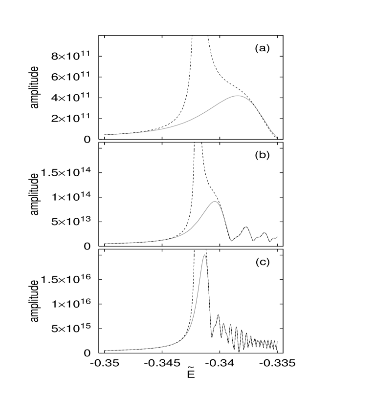
Figure 21: Uniform approximation to the contribution of the considered bifurcation scenario to the density of states for three different values of the magnetic field strength: (a) $\gamma=10^{-10}$, (b) $\gamma=10^{-12}$, (c) $\gamma=10^{-14}$. Solid curves: Uniform approximation, dashed curves: Gutzwiller’s trace formula.

The uniform approximation was calculated for the same values of the magnetic field strength as was the local approximation. The results are displayed in figure 21. They are finite at the bifurcation energies and do indeed reproduce the results of Gutzwiller’s trace formula as the distance from the bifurcation increases. Even the complicated oscillatory structures in the density of states which are caused by interferences betweeen contributions from different periodic orbits are perfectly reproduced by our uniform approximation. We can also see that the higher the magnetic field strength, the farther away from the bifurcation energies is the asumptotic (Gutzwiller) behavior acquired. In fact, for the largest field strength $\gamma=10^{-10}$ the asymptotic regime is not reached at all in the energy range shown. This behavior can be traced back to the fact that, due to the scaling properties of the Diamagnetic Kepler Problem, the scaling parameter $\gamma^{-1/3}$ plays the rôle of an effective Planck’s constant, therefore the lower $\gamma$ becomes, the more accurate the semiclassical approximation will be.

6 Summary

We have shown that in generic Hamiltonian systems bifurcations of ghost orbits can occur besides the bifurcations of real orbits. If they occur in the neighborhood of a bifurcation of a real orbit, they produce signatures in semiclassical spectra in much the same way as bifurcations of real orbits and therefore are of equal importance to a semiclassical understanding of the quantum spectra. Furthermore, we have shown that the technique of normal form expansions traditionally used to construct uniform approximations taking account of bifurcations of real orbits only can be extended to also include the effects of ghost orbit bifurcations. Thus, normal form theory offers techniques which will allow us, at least in principle, to calculate uniform approximations for arbitrarily complicated bifurcation scenarios.

The effects ghost orbit bifurcations exert on semiclassical spectra were illustrated by way of example of the period-quadrupling bifurcation of the balloon-orbit in the Diamagnetic Kepler Problem. This example was chosen mainly because of its simplicity, because the balloon-orbit is one of the shortest periodic orbits in the Diamagnetic Kepler Problem, and the period-quadrupling is the lowest period-$m$-tupling bifurcation that can exhibit the island-chain-bifurcation typical of all higher $m$. We can therefore expect ghost orbit bifurcations also to occur for longer orbits and in connection with higher period-$m$-tupling bifurcations. This conjeture is confirmed by the discussion of the various bifurcation scenarios described by the higher-order normal form (45), which reveals ghost orbit bifurcations close to a period-quadrupling in three out of four possible cases. Thus, ghost orbit bifurcations will be a common occurence in generic Hamiltonian systems. Their systematic study remains an open problem for future work.

Figure 1: The balloon orbit (a) in semiparabolical and (b) in cylindrical coordinates at a scaled energy of $\tilde{E}=-0.34$.

Tr M
	$\mathsf{\tilde{E}}$

Figure 2: The trace of the monodromy matrix of the balloon orbit. The zero at $\tilde{E}_{c}=-0.342025$ indicates the occurence of the period-quadrupling bifurcation.

Figure 3: Real satellite orbits involved in the period-quadrupling bifurcation of the balloon orbit at scaled energies of (a) $\tilde{E}=-0.34$ and (b) $\tilde{E}=-0.3418$. Solid curve: stable satellite, dashed curve: unstable satellite; for comparison: dotted curve: balloon orbit.

Figure 4: Ghost orbits at scaled energy of $\tilde{E}=-0.343$. Solid and dotted curves: stable and unstable ghost satellite orbits created in the period-quadrupling of the balloon orbit at $\tilde{E}_{c}=-0.342025$. Dashed curve: additional ghost orbit created in the ghost bifurcation at $\tilde{E}_{c}^{\prime}=-0.343605$.

Figure 5: Ghost orbits at scaled energy of $\tilde{E}=-0.344$. Solid and dashed curves: Asymmetric ghost orbits created in the ghost bifurcation at $\tilde{E}_{c}^{\prime}=-0.343605$ (real parts coincide). Dotted curve: Unstable ghost satellite orbit created in the period quadrupling of the balloon orbit at $\tilde{E}_{c}=-0.342025$.

Figure 6: Actions, orbital periods and traces of the monodromy matrices of the orbits involved in the bifurcation scenario as functions of the scaled energy $\tilde{E}=\gamma^{-2/3}E$. Solid curves: real orbits, dashed curves: ghost orbits symmetric with respect to complex conjugation, dotted curves: asymmetric ghost orbits.

Figure 8: The dependence of the radial coordinate $I_{\sigma}$ on $\zeta$ illustrates the bifurcations orbits undergo. Only orbits having a fixed $\sigma$ are included in these plots: (a) $\varrho_{\sigma}>0$, (b) $\varrho_{\sigma}<0$. Solid curves: real orbits, dashed curves: ghost orbits symmetric with respect to complex conjugation, dotted curves: a pair of complex conjugate ghosts.

Figure 10: Plots of the normal form illustrating the bifurcation scenario of case 1. Solid curve: $\sigma=+1$, dashed-dotted curve: $\sigma=-1$.

Figure 11: Plots of the normal form illustrating the bifurcation scenario of case 2.

Figure 12: Plots of the normal form illustrating the bifurcation scenario of case 3.

Figure 13: Plots of the normal form illustrating the bifurcation scenario of case 4.

Figure 15: Plots of the normal form illustrating the bifurcation scenario described by the normal form (49).

Figure 16: Bifurcation scenario described by the normal form (49) in the case $|a|>|b|$ and $c<0$.

$\mathsf{Re\,\Delta\tilde{S}/2\pi}$
	$\mathsf{\tilde{E}}$

$\mathsf{Im\,\Delta\tilde{S}/2\pi}$
	$\mathsf{\tilde{E}}$

Figure 17: Comparison of the action differences calculated from the normal form (49) with parameter values (83) to the actual action differences. Solid curves: numerically calculated values, dashed curves: stationary values of the normal form.

$\mathsf{Re\,(Tr\;M-2)}$
	$\mathsf{\tilde{E}}$

$\mathsf{Im\,(Tr\;M-2)}$
	$\mathsf{\tilde{E}}$

Figure 18: Comparison of the traces of the monodromy matrices calculated from the normal form (49) with parameter values (83) to the actual traces. Solid curves: numerically calculated traces, dashed curves: Hessian determinants of the normal form.

Figure 20: Values of the normal form parameters calculated from (95) which were used for the uniform approximation.

References

- [1] Arnold V I: Mathematical methods of classical mechanics (New York: Springer 1989)
- [2] Arnold V I, Kozlov V V, and Neishadt A I in Dynamical Systems III, Encyclopedia of Mathematical Sciences, vol. 3, ed. V. I. Arnold (Berlin: Springer 1988)
- [3] Artuso R, Aurell E, and Cvitanović P: Nonlinearity 3 (1990), 325 and 361
- [4] Bartsch T, Main J, and Wunner G: J. Phys. A 32 (1999), 3013
- [5] Birkhoff G D: Dynamical Systems. AMS Colloquium Publications vol. IX (Providence, RI, 1927, 1966)
- [6] Cvitanović P, Eckhardt B: Phys. Rev. Lett. 63 (1989), 823
- [7] Einstein A: Verh. Dtsch. Phys. Ges. 19(1917),82
- [8] Feynman R P: Rev. Mod. Phys. 20 (1948), 367
- [9] Friedrich H and Wintgen D: Phys. Rep. 183 (1989), 37
- [10] Goldstein H: Classical Mechanics (Reading, Mass.: Addison-Wesley 1959)
- [11] Gustavson F: Astron. J. 71 (1966), 670
- [12] Gutzwiller M C: J. Math. Phys. 8 (1967), 1979 and J. Math. Phys. 10 (1969), 1004
- [13] Gutzwiller M C: J. Math. Phys. 11 (1970), 1791
- [14] Gutzwiller M C: J. Math. Phys. 12 (1971), 343
- [15] Gutzwiller M C: Physica D 5 (1982), 183
- [16] Gutzwiller M C: Chaos in Classical and Quantum Mechanics (Berlin: Springer 1990)
- [17] Hasegawa H, Robnik M, and Wunner G: Prog. Theor. Phys. Supp. 98 (1989), 198
- [18] Kuś M, Haake F, and Delande D: Phys. Rev. Lett. 71 (1993), 2167
- [19] Mao J-M and Delos J B: Phys. Rev. A 45 (1992), 1746
- [20] Main J and Wunner G: Phys. Rev. A 55 (1997), 1743
- [21] Main J and Wunner G: Phys. Rev. E 57 (1998), 7325
- [22] Main J, Mandelshtam V A, Wunner G, and Taylor H S: Nonlinearity 11 (1998), 1015
- [23] Meyer K R: Trans. AMS 149 (1970), 95
- [24] Ozorio de Almeida A M and Hannay J H: J. Phys. A 20 (1987), 5873
- [25] Ozorio de Almeida A M: Hamiltonian Systems: Chaos and Quantization (Cambridge University Press 1988)
- [26] Peters A, Jaffé C, and Delos J: Phys. Rev. Lett. 73 (1994), 2825
-
[27]
Poston T and Stewart I N:
Catastrophe Theory and its Applications.
(London: Pitman 1978) - [28] Sadovskií D A, Shaw J A, and Delos J B: Phys. Rev. Lett. 75 (1995), 2120
- [29] Sadovskií D A and Delos J B: Phys. Rev. E 54 (1996), 2033
- [30] Schomerus H and Sieber M: J. Phys. A 30 (1997), 4537
- [31] Schomerus H: Europhys. Lett. 38 (1997), 423
- [32] Schomerus H and Haake F: Phys. Rev. Lett. 79 (1997), 1022
- [33] Schomerus H: J. Phys. A 31 (1998),4167
- [34] Schulman L S: Techniques and Applications of Path Integration (New York: John Wiley & Sons 1981)
- [35] Sieber M: J. Phys. A 29 (1996), 4715
- [36] Sieber M and Schomerus H: J. Phys. A 31 (1998), 165
- [37] Sirovich L: Techniques of Asymptotic Analysis (New York: Springer 1971)
- [38] Watanabe S in Review of Fundamental Processes and Applications of Atoms and Ions, ed. C. D. Lin (Singapore: World Scientific 1993)
- [39] Wintgen D: J. Phys. B 20 (1987), L511