Invariant sets for discontinuous parabolic area-preserving torus maps

Abstract

We analyze a class of piecewise linear parabolic maps on the torus, namely those obtained by considering a linear map with double eigenvalue one and taking modulo one in each component. We show that within this two parameter family of maps, the set of noninvertible maps is open and dense. For cases where the entries in the matrix are rational we show that the maximal invariant set has positive Lebesgue measure and we give bounds on the measure. For several examples we find expressions for the measure of the invariant set but we leave open the question as to whether there are parameters for which this measure is zero.

Revised version

PACS: 05.45.+b

Keywords: Parabolic maps on the torus, non-invertibility, measure of invariant set, Interval translation map

1 Introduction

We consider a class of maps of the torus $X=[0,1]^{2}$ of the form

$$\begin{array}[]{l}x^{\prime}=ax+by~{}(\bmod~{}1)\\ y^{\prime}=cx+dy~{}(\bmod~{}1)\end{array}$$ (1)

where $(x,y)\in[0,1]^{2}$. This can be thought of as a map $f=g\circ M$ where

$$M=\left(\begin{array}[]{cc}{a}&{b}\\ {c}&{d}\end{array}\right)$$

(we also write $M=(a,b;c,d)$ for convenience) and $g(x)=x-\lfloor x\rfloor$ is a map that takes modulo $1$ in each component. Although such maps are linear except at the discontinuity induced by the map $g$, their dynamical behaviour can be quite complicated. Depending on the eigenvalues $\lambda_{1,2}$ of $M$ we refer to the map as elliptic ($\lambda_{1}=\overline{\lambda}_{2}\neq\lambda_{1}$), hyperbolic ($\lambda_{1}>\lambda_{2}$) or parabolic ($\lambda_{1}=\lambda_{2}$). In this paper we focus on the area-preserving parabolic case with determinant $ad-bc=1$ and trace $a+d=2$. Such maps arise naturally on examining linear maps with a periodic overflow. In particular, suppose that one would like to iterate a matrix using a digital representation with very small discretization error but a finite range which we set to be $(0,1)$. If the calculation overflows such that the fractional part remains, we will get the map (1) (compare, for example, with [4]).

In this case $f$ is a piecewise continuous map of ${\bf T}^{2}={\bf R}^{2}/{\bf Z}^{2}$ to itself that is area-preserving and such that the linearization is at almost every point in ${\bf T}^{2}$ is $M$. This matrix has two eigenvalues equal to one. The map is continuous everywhere on the torus except on a one-dimensional discontinuity $D$ in ${\bf T}^{2}$. The behaviour of $f$ on $D$ does not affect a full measure set of $X$.

Parabolic area-preserving maps are not typical in the set of almost-everywhere linear maps on the torus [5]. However, their dynamical properties are of a particular interest, since such maps can be considered as an interpolating case between the hyperbolic maps ($|t|>2$) and the elliptic maps ($|t|<2$) in the area-preserving case. They are in some sense generalisations of interval exchange maps [13, 16, 11], piecewise rotations [8, 4] and interval translation maps [6, 15] to two dimensions. In fact, in Section 3 and the subsequent sections, our results use the fact that for rational coefficients of $M$ the map (1) may be decomposed into a one-parameter family of 1 dimensional interval translation maps.

Hyperbolic area-preserving maps are characterized by a positive Liapunov exponents, and are often studied as model chaotic area-preserving dynamical systems (see eg. [5, 14] and the Baker’s transformation). Elliptic area-preserving maps correspond (in an appropriate eigenbasis) to rigid rotation, where the presence of a discontinuity caused by $g$ will lead to very complicated dynamics [2, 3, 9, 4]. The elliptic–hyperbolic transition for the linear maps on the torus was studied by Amadasi and Casartelli [1], while certain properties of linear parabolic maps were analyzed in [17]. In particular, a generic parabolic map displays some sort of sensitive dependence on initial conditions. However, this property is not related to the Lyapunov exponents (which are always zero for parabolic maps), but is due to the discontinuity of the map.

1.1 Summary of main results

We parametrize the set of parabolic area-preserving maps by $A$ and $\alpha$, namely

$$\begin{array}[]{l}\left(\begin{array}[]{c}{x^{\prime}}\\ {y^{\prime}}\end{array}\right)=f\left(\begin{array}[]{c}{x}\\ {y}\end{array}\right)=\left(\begin{array}[]{c}{(1+A)x+\frac{A}{\alpha}y~{}(\bmod 1)}\\ {-\alpha Ax+(1-A)y~{}(\bmod 1)}\end{array}\right)\end{array}.$$ (2)

Section 2 characterises (in Theorem 1) the open dense set of $(A,\alpha)$ such that the mapping (2) is not invertible and discuss some properties of the invertible maps. Section 3 examines properties of the maximal invariant set [17]

$$X^{+}=\bigcap_{n=0}^{\infty}f^{n}(X)$$

which by the previous result is strictly smaller than $X$ for most $(A,\alpha)$. Note that any $A\subset X$ with $f(A)=A$ will have $A\subset X^{+}$ and so in this sense the set is maximal.

We say a map (2) is semirational if $\alpha$ is rational. It is rational if both $A$ and $\alpha$ are rational. If $f$ is not semirational we say it is irrational. Note that the map is rational if and only if $a$, $b$, $c$ and $d$ are rational.

We investigate the two dimensional Lebesgue measure $\ell(\cdot)$ of this set, showing in Theorem 3 that for rational parabolic maps we have $\ell(X^{+})>0$. We give explicit lower and upper bounds for $\ell(X^{+})$ depending on $A$ and $\alpha$.

We discuss two particular examples of rational maps where we can compute $\ell(X^{+})$, namely with $A=\frac{1}{2}$ and $\alpha=1$ or $\frac{1}{2}$. In the former case we show that $\ell(X^{+})=\frac{1}{2}$ and in the latter case we show that $\ell(X^{+})=\frac{1}{2}-\frac{\sqrt{3}\pi}{72}-\frac{1}{8}\ln 3\sim 0.28710$. In some special cases, e.g., $-1\leq\alpha<0,~{}|A|\leq 1$ and $A=1,~{}0<\alpha<1$ , we can compute $X^{+}$, and thus we can obtain exact values of $\ell(X^{+})$. Other than these cases we have not been able to compute exact values of $\ell(X^{+})$ other than by numerical approximation, even for rational $A$ and $\alpha$. We suspect that for many $\alpha>0$ and $A>0$ (both irrational) then $\ell(X^{+})=0$, whereas $\ell(X^{+})>0$ for $\alpha$ rational. Section 4 briefly discusses examples of nonlinear parabolic maps, and we conclude with some remarks on open problems in Section 5.

2 Invertibility of linear maps on the torus

Consider a matrix $M$ corresponding to a parabolic map on the torus (1). Apart from the special horocyclic [7] cases

$$\left(\begin{array}[]{cc}{1}&{B}\\ {0}&{1}\end{array}\right)~{}~{}~{}~{}\left(\begin{array}[]{cc}{1}&{0}\\ {B}&{1}\end{array}\right),$$ (3)

any such matrix can be written in the form

$$M=M_{A,\alpha}=\left(\begin{array}[]{cc}{1+A}&{A/\alpha}\\ {-\alpha A}&{1-A}\end{array}\right),$$ (4)

where $A$ and $\alpha$ are real parameters. Observe that the cases $\alpha,A\rightarrow 0$ (with $A/\alpha$ held constant) and $\alpha\rightarrow\infty$, $A\rightarrow 0$ (with $\alpha A$ held constant) correspond to the cases (3). Observe that

$$M_{A,\alpha}^{-1}=M_{-A,\alpha},$$

and if $S(x,y)=(y,x)$ is transposition then $S^{2}=I$ and

$$SM_{A,\alpha}=M_{-A,1/\alpha}S.$$

Moreover, in the absence of the rounding $g$ we have

$$M_{A,\alpha}^{p}=M_{pA,\alpha}$$

for any $p\in{\bf Z}$.

2.1 Noninvertibility of generic parabolic maps

The next lemma gives necessary and sufficient conditions that (1) is invertible (ignoring points that land on the discontinuity). We say the map is invertible if there is a full measure subset on which it is invertible. Since the mapping is a composition of an invertible linear map and a discontinuous map that maps open sets to open sets, both of which preserve Lebesgue measure, a map is non-invertible if and only if there is an open set of $(x,y)$ that has two or more preimages. Let $a,b,c,d$ be defined as previously.

Lemma 1

Any map (1) with $ad-bc=1$ will be noninvertible on an open set if and only if there are $(K,L)\in{\bf Z}^{2}\setminus(0,0)$ integers such that

$$|Kc-La|<1~{}\mbox{ and }~{}|Kd-Lb|<1.$$

Proof      Suppose that we have $(x,y)$ and $(u,v)\in[0,1)^{2}$ such that $(x,y)\neq(u,v)$ but $f(x,y)=f(u,v)$. Then there is $(K,L)\in{\bf Z}^{2}\setminus(0,0)$ such that $ax+by=au+bv+K$ and $cx+dy=cu+dv+L$. These hold if and only if

$$a(x-u)+b(y-v)=K~{}\mbox{ and }~{}c(x-u)+d(y-v)=L.$$

Using the fact that $a,b,c,d$ are non-zero and $ad-bc=1$ this implies that this holds if and only if

$$x-u=Kc-La~{}\mbox{ and }~{}y-v=Kd-Lb.$$

Thus the mapping is many-to-one if and only if there are $K$ and $L$ such that

$$|Kc-La|<1~{}\mbox{ and }~{}|Kd-Lb|<1$$

and the result follows.  

Remark 1

It is quite possible that there are simultaneously many solutions to the inequalities of Lemma 1; for example, near $A=-1$ and $\alpha$ large one can find arbitrarily large numbers of integers $(K,L)$ satisfying both inequalities.

Using the previous Lemma we obtain the main result of this section.

Theorem 1

The only invertible parabolic maps $f$ have $M$ equal to one of

$$\left(\begin{array}[]{cc}{k}&{-(k-1)^{2}/l}\\ {l}&{2-k}\end{array}\right),~{}~{}\left(\begin{array}[]{cc}{2+l}&{-k}\\ {(l+1)^{2}/k}&{-l}\end{array}\right),~{}~{}\left(\begin{array}[]{cc}{1}&{b}\\ {0}&{1}\end{array}\right)~{}~{}\mbox{ or }~{}~{}\left(\begin{array}[]{cc}{1}&{0}\\ {b}&{1}\end{array}\right),$$

where $(k,l)$ are integers and $b$ is real.

Proof      The square $V_{\epsilon}=(-1-\epsilon,1+\epsilon)^{2}$ is a convex region symmetrical about the origin with area $4(1+\epsilon)^{2}$. A variant of Minkowski’s theorem [10, Thm 447] says that for any $\epsilon>0$ there will be a point on the lattice $\Lambda=\{(Kc-La,Kd-Lb)~{}:~{}(K,L)\in{\bf Z}^{2}\}$ other than zero inside $V_{\epsilon}$, if the lattice has determinant $\Delta=ad-bc\geq 1$. Taking the limit $\epsilon\rightarrow 0$ and using compactness we see that there must be a point $(\kappa,\lambda)\in\Lambda$ other than zero in $\overline{V_{0}}$.

If there is a lattice point $(\kappa,\lambda)$ in the interior of $V_{0}$, we are done. If not, assume without loss of generality that $(\kappa,\lambda)=(1,y)$ with $|y|\leq 1$. Thus exactly one point in the line segment from (but not including) $(-1,1-y)$ to $(0,1)$ that is in the lattice (one can generate the same lattice by adding multiples of $(1,y)$ to any lattice point generating the lattice with $(1,y)$). Therefore there will be a point in the lattice in the interior of $V_{0}$ unless this other point is $(0,1)$. Therefore (considering the other case by interchanging $x$ and $y$) there will be integers $K$ and $L$ such that either

$$(Kc-La=1~{}~{}\mbox{ and}~{}~{}Kd-Lb=0)~{}~{}~{}\mbox{ or }~{}~{}~{}(Kc-La=0~{}~{}\mbox{and}~{}~{}Kd-Lb=1).$$

Thus, in the invertible case the matrix $M$ is determined by which of these cases occurs. One can easily solve to show that either of these cases can occur. If $k=1$ or $l=-1$ then the other (horocyclic) cases occur.  

It follows from this result that most parabolic maps are noninvertible in the following sense:

Corollary 1

The set of noninvertible maps is open and dense within the set of parabolic maps.

Because the $(\bmod~{}1)$ map $g$ commutes with integer matrix and $g^{2}=g$, all conjugations of parabolic maps with integer coefficients by automorphisms of the torus ${\bf T}^{2}$ remain integer parabolic maps. For an integer parabolic map with rational $\alpha=r/s$, where $(r,~{}s)=1$, since there exist $m,~{}n\in{\bf Z}$ such that $mr+ns=1$, there exists an automorphism whose $GL(2,{\bf Z})$ matrix has bottom row $(r,~{}s)$. Conjugation by this automorphism gives a parabolic map whose matrix has bottom row $(0,~{}*)$. Since conjugation preserves integrality, trace and determinant, the resulting matrix must be of the form $(1,~{}B;~{}0,~{}1)$ for some $B$. Therefore we conclude that all parabolic maps with integer coefficients can be reduced to one of the horocyclic cases.

3 Maximal invariant sets

By Poincaré recurrence the maximal invariant set $X^{+}=X$ (up to a set of zero measure) if and only if $f$ is invertible at almost every point. In fact the maximal invariant set $X^{+}$ is an upper semicontinuous function of the system parameters $A,\alpha$ in the Hausdorff metric. However, the measure (and dimension) of $X^{+}$ can (and does) change discontinously with parameters; see Proposition 1.

We now consider the structure of $X^{+}$ for the semirational case (ie $\alpha$ rational). Consider the family of lines $L_{B}$ defined by

$$y=B-\alpha x$$

with $B$ a fixed real number. projected onto the torus by taking modulo $1$ in $x$ and $y$. This can be thought of as the set

$$L_{B}=\{(x,y)~{}:~{}y=B+K-\alpha(x+L)~{}~{}\mbox{with}~{}~{}(K,L)\in{\bf Z}^{2}\}\cap X.$$

Note that if

$$y=B+K-\alpha(x+L)$$

with $L$ and $K$ integers such that $x,y$ in $[0,1]$ then $y^{\prime}=-\alpha Ax+(1-A)(B+K-\alpha(x+L)+N$ and $x^{\prime}=(1+A)x+A/\alpha(B+K-\alpha(x+L))+M$ with $M,N$ integers. Rearranging this we have

$$y^{\prime}=B+(K+M+N)-\alpha(x+L)$$

and so the family of lines $L_{B}$ is invariant under the map for any given $B$. We define the maximal invariant set within $L_{B}$ as

$$X_{B}^{+}=X^{+}\cap L_{B}.$$

3.1 Semirational and rational parabolic maps

For semirational maps ($\alpha=r/s>0$) and for any given value of $B$ the set $L_{B}$ consists of $r+s$ (or exceptionally $r+s-1$ if it contains the origin) intervals that are parallel to the eigenvector $v=(1,-\alpha)$ of the matrix $M$. We can parametrise any particular $L_{B}$ by $\theta\in[0,s)$. We will consider $\alpha>0$ from here on. More precisely we re-parametrize $X$ by

$$\begin{array}[]{l}x=\theta-[\theta]\\ y=B-\alpha\theta-[B-\alpha\theta]\end{array}$$ (5)

For $\theta\in[0,s)$ and $B\in[\frac{s-1}{s},1)$ the mapping $(x,y)\leftrightarrow(\theta,B)$ is one-to-one and has unit Jacobian everywhere.

Since each $L_{B}$ is invariant the maximal invariant set must nontrivially intersect $L_{B}$ and so no single trajectory is dense in $X^{+}$. In this case we need to approximate $X^{+}$ using a distribution of trajectories on a dense set of lines.

The relation between $\theta$ and $x$ is $x=\theta-[\theta].$ The variable $y$ is related to $\theta$ and $B$ by the relation $y=B-\alpha\theta-[B-\alpha\theta]$. So the point $(\theta,B)$ maps to

$$(\theta^{\prime},B^{\prime})=(\theta+AB/\alpha-A[\theta]-A/\alpha[B-\alpha\theta],B)$$

since

$$\left(\begin{array}[]{c}{\theta^{\prime}}\\ {v}\end{array}\right) = \left(\begin{array}[]{cc}1+A&A/\alpha\\ -A\alpha&1-A\end{array}\right)\left(\begin{array}[]{c}\theta-[\theta]\\ B-\alpha\theta-[B-\alpha\theta]\end{array}\right)+\left(\begin{array}[]{c}[\theta]\\ \left[B-\alpha\theta\right]\end{array}\right)$$

$$= \left(\begin{array}[]{c}\theta+AB/\alpha-A[\theta]-A/\alpha[B-\alpha\theta]\\ -\alpha\theta+B-AB+A\alpha[\theta]+A[B-\alpha\theta]\end{array}\right).$$

We have added integers $[\theta]$ and $[B-\alpha\theta]$ so that $\theta^{\prime}\in[0,s)$ and $v=B-\alpha\theta$ (see eg [17]).

Thus the action of the map (1) on the coordinate $\theta$ is simply

$$\theta^{\prime}=T_{B}(\theta)=\left(\theta+\frac{s}{r}AB-A[\theta]-A\frac{s}{r}[B-\frac{r}{s}\theta]\right)~{}(\bmod s).$$ (8)

Because the variable $B\in[\frac{1-s}{s},1)$ is invariant during the dynamics it is treated as a parameter. Again, the slope of these 1D maps is equal to one implying that all Liapunov exponents are zero.

In the case of a rational map, ie where both $A=p/q$ and $\alpha=r/s$ are rational with $(r,s)=(p,q)=1$ we can understand a lot about the mapping $T$ using the following factor map. Let

$$\pi(\theta)=\theta-\frac{1}{qr}[qr\theta]$$

be a projection of $I=[0,s)$ onto $J=[0,\frac{1}{qr})$: this maps $qrs$ points onto one point.

Lemma 2

If $A=\frac{p}{q}$ and $\alpha=\frac{r}{s}$ then the diagram

$$\begin{array}[]{rcl}I&\stackrel{{\scriptstyle T_{B}}}{{\rightarrow}}&I\\ \pi\downarrow&&\downarrow\pi\\ J&\stackrel{{\scriptstyle S_{B}}}{{\rightarrow}}&J\end{array}$$

commutes where

$$S_{B}(\psi)=\psi+\frac{sp}{rq}B~{}(\bmod\frac{1}{qr})$$

is a rotation. In other words $T_{B}$ has a factor that is a rotation.

Proof      For these assumptions we can write (8) as

$$\theta^{\prime}=\left(\theta+\frac{sp}{rq}B-\frac{p}{q}[\theta]-\frac{ps}{qr}[B-\frac{r}{s}\theta]\right)~{}(\bmod s).$$ (9)

Defining $\psi=\pi(\theta)$ and $\psi^{\prime}=\pi(\theta^{\prime})$, note that

$$\psi^{\prime}=\psi+C~{}(\bmod\frac{1}{qr})$$

where $C=\pi(AB/\alpha)=\pi(\frac{sp}{rq}B)$.  

Since $S_{B}$ is invertible, $\cap_{n=0}^{\infty}S^{n}(J)=J$. The map $\pi$ maps $M=qrs$ points to one point and so $\pi^{-1}$ must be understood as a set-valued function. We have

$$\pi\pi^{-1}(\psi)=\psi,~{}~{}\pi T(\theta)=S\pi(\theta)$$

for all $\psi\in J$ and $\theta\in I$, while for any set $K\subset I$

$$\pi^{-1}\pi K\supseteq K.$$

Let

$$N(\psi) = \{\theta\in X^{+}_{B}~{}:~{}\pi(\theta)=\psi\}=\pi^{-1}(\psi)\cap X_{B}^{+}$$

be the set of $\theta\in X_{B}^{+}$ with $\pi(\theta)=\psi$ (we suppress the dependence of $S$ and $T$ on $B$ for the next result).

Lemma 3

For any $\psi\in J$, the set $N$ satsifies

$$N(S(\psi))=T(N(\psi)).$$

Proof      To show that $T(N(\psi))\subseteq N(S(\psi))$, note that

$$T(N(\psi)) \subseteq \pi^{-1}\pi T(N(\psi))=\pi^{-1}S\pi(N(\psi))$$

$$= \pi^{-1}S\pi(\pi^{-1}(\psi)\cap X_{B}^{+})$$

$$\subseteq \pi^{-1}S(\psi))\cap X_{B}^{+}$$

$$= N(S(\psi)).$$

For the other direction, suppose that $\theta\in N(S(\psi))$ and so $\pi(\theta)=S(\psi)$ and $\theta\in\cap_{n\geq 0}T^{n}(I)$. In particular, $\theta=T(\theta^{\prime})$ for some $\theta^{\prime}$. Now $\pi(\theta)=\pi T(\theta^{\prime})=S\pi(\theta^{\prime})$ and so $S(\psi)=S\pi(\theta^{\prime})$. Invertibility of $S$ gives $\psi=\pi(\theta^{\prime})$ and so $\theta^{\prime}\in N(\psi)$. Hence

$$T(N(\psi))\supseteq N(S(\psi))$$

and we have the result.  

The previous Lemma relies crucially on the fact that $S$ is invertible. The next result implies that the number of points in $N$ is a constant almost everywhere. Let

$$\hat{N}=|N(\psi)|$$

be the cardinality of $N(\psi)$.

Lemma 4

If $B$ is irrational then $\hat{N}$ is constant for a set of $\psi$ with full Lebesgue measure.

Proof      It is a standard result that $S_{B}$ is ergodic for Lebesgue measure if and only if $B$ is irrational. If we look at the set of $\psi$ that give a certain value of $N(\psi)$ this is invariant and therefore must have Lebesgue measure $0$ or $1$.  

One consequence of this is that the measure of $X_{B}^{+}$ can only take a finite number of values. We write $\hat{N}(B)$ to show the dependence on $B$ explicitly.

Theorem 2

Suppose that $A=p/q$ and $\alpha=r/s$. For Lebesgue almost all $B$ we have

$$\ell(X_{B}^{+})=\frac{\hat{N}(B)}{qr}$$

where $\hat{N}(B)$ is an integer and $1\leq\hat{N}(B)\leq qrs$. If there is an interval on which $T$ has $L$ preimages, then

$$\hat{N}(B)\leq qrs+1-L.$$

Proof      As preimages of $\pi^{-1}(J)$ are disjoint and all have length $\frac{1}{qr}$ we compute

$$\ell(X_{B}^{+})=\sum_{k=1}^{\hat{N}(B)}\frac{1}{qr}=\frac{\hat{N}(B)}{qr}.$$

Note that $\hat{N}(B)$ must take an integer value less than or equal to $qrs$, being the number of preimages $\pi^{-1}(\psi)$.

Since $T$ will be invertible on $X_{B}^{+}$, if there is an interval with more than one preimage, only one of these will be in $X_{B}^{+}$ and hence $\hat{N}(B)\leq qrs+1-L$ where $L$ is the number of preimages.  

We can now prove the main result in this section.

Theorem 3

Suppose that $\alpha=r/s$ and $A=p/q$ are both rational, with $(r,s)=(p,q)=1$. Then the maximal invariant set $X^{+}$ has Hausdorff dimension $2$ and positive Lebesgue measure, more precisely, if there is an open set on which $f$ has $K$ preimages then

$$\frac{1}{qrs}\leq\ell(X^{+})\leq 1-\frac{K-1}{qrs}.$$

Proof      Note that under the hypotheses of the theorem,

$$\ell(X^{+}) = \int_{B\in[1-\frac{1}{s})}\int_{s\in X_{B}^{+}}\,d\theta\,ds$$

$$= \int_{B\in[1-\frac{1}{s})}\ell(X_{B}^{+})\,ds.$$

Upon integrating the estimates in Theorem 2 we obtain the result.  

We can characterise the dynamics on the lines $L_{B}$ in the following way:

Corollary 2

For any rational map, almost all $B$ and all $x\in L_{B}$, $\omega(x)$ consists of a set with positive one-dimension measure in $L_{B}$. Conversely, for a countable set of $B$ and all $x\in L_{B}$, the trajectory going through $x$ is eventually periodic.

Proof      In the proof of Theorem 3, the reduced map $S_{B}$ will be an irrational rotation for all irrational $B$ and a rational rotation for all rational $B$. The result follows.  

Density of irrational $B$ simply implies the following result for the original map.

Corollary 3

For any rational parabolic map, the preimages of the discontinuity are dense in $X^{+}$.

We do not have a precise analytical expression for $\ell(X^{+})$ even for rational parabolic maps. Numerically one can approximate the measure and obtain various values of $\ell(X^{+})$; see for example Table 1. In certain simple cases one can obtain exact values of $\ell(X^{+})$ by constructing the maximal invariant set explicitly.

Proposition 1

One can compute

$$\ell(X^{+})=\left\{\begin{array}[]{ll}1&\mbox{ if the map is invertible,}\\ \alpha&\mbox{ if $A=1$ and $0<\alpha\leq 1$,}\\ \alpha^{-1}&\mbox{ if $A=-1$ and $\alpha\geq 1$, and}\\ |A\alpha|&\mbox{ if $0<A\leq 1$ and $-1\leq\alpha<0$}.\end{array}\right.$$

The invertible case is trivial, while the cases where $A=1$ follow because the map reduces to an invertible map on a strip height $\alpha$. The appendix gives a constructive proof for the case $0<A\leq 1$, $-1\leq\alpha<0$. Because $f_{-A,-1}$ is conjugate to $f_{A,-1}$ by interchanging $x$ and $y$ we have

$$\ell(X^{+})=\left\{\begin{array}[]{cc}|A|~{},&~{}~{}0<|A|\leq 1~{},\alpha=-1\\ 1~{},&~{}~{}A=0~{},\alpha=-1.\end{array}\right.$$

Note in particular that there is a discontinuity in $\ell(X^{+})$ at $(\alpha,A)=(1,0)$.

The following examples (especially that in Section 3.3) show that a general expression, if it can be obtained, is likely to be non-trivial.

$$\begin{array}[]{l|llll}A&\alpha=2/3&1/2&1/3&1/5\\ \hline\cr 1/4&0.261&0.337&0.251&0.196\\ 1/3&0.235&0.326&0.265&0.199\\ 2/3&0.215&0.342&0.257&0.149\\ 5/4&0.628&0.626&0.419&0.252\\ 3/2&0.338&0.562&0.505&0.303\end{array}$$

Table 1: Numerically obtained approximate values of $\ell(X^{+})$ for a number of rational parabolic maps.

3.2 Example I

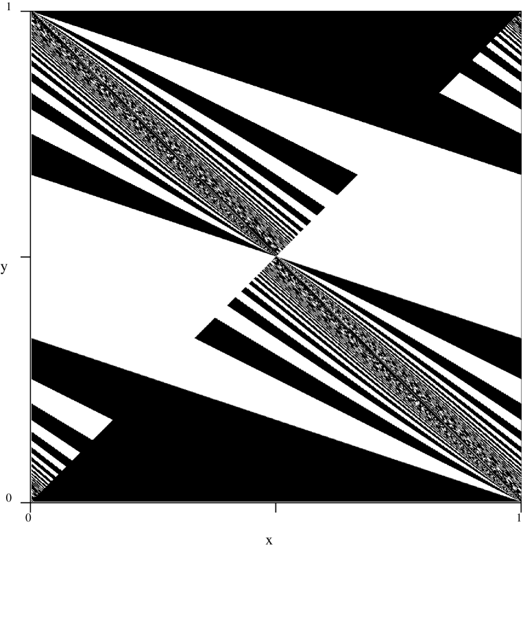
Figure 1: The black region shows the maximal invariant set $X^{+}$ for the map (10) where $A=1/2$ and $\alpha=1$. Observe the symmetry of the black and white regions indicating that $\ell(X^{+})=\frac{1}{2}$.

The simplest nontrivial rational map is defined by $A=1/2$ and $\alpha=1$. In this case, we can approximate the maximal invariant set numerically as in Figure 1. The map in this case is

$$\begin{array}[]{l}x^{\prime}=\frac{3}{2}x+\frac{1}{2}y~{}(\bmod 1)\\ y^{\prime}=-\frac{1}{2}x+\frac{1}{2}y~{}(\bmod 1)\end{array}$$ (10)

where $(x,y)\in X=[0,1]^{2}$. In this case, as noted in [17], there appears to exist a symmetry between $X^{+}$ and its complement. In fact, we can use the results in Section 3.1 to get the result directly.

Proposition 2

For the map (10) with $A=\frac{1}{2}$ and $\alpha=1$, we have $\ell(X^{+})=\frac{1}{2}$.

Proof      Note that $r=s=p=1$ and $q=2$. Moreover, on $L_{B}$ the map (8) can be written

$$\theta^{\prime}=h(\theta)=\theta+\frac{B}{2}-\frac{1}{2}[B-\theta]~{}(\bmod 1)$$

and this map is two-to-one on an open set of $\theta$ for almost all $B$. Therefore, for almost all $B$, the upper and lower bounds of Theorem 2 agree and

$$\ell(X_{B}^{+})=\frac{1}{2}$$

for almost all $B$. This implies that $\ell(X^{+})=\frac{1}{2}$.  

3.3 Example II

We now consider the case $A=\alpha=1/2$; this shows that $\ell(X^{+})$ may be irrational for a rational map. In this case the map is

$$\begin{array}[]{l}x^{\prime}=\frac{3}{2}x+y~{}(\bmod 1)\\ y^{\prime}=-\frac{1}{4}x+\frac{1}{2}y~{}(\bmod 1)\end{array}$$ (11)

On the invariant lines $L_{B}$ with $B\in[\frac{1}{2},1)$ (11) reduces to (8) with $\theta\in[0,2)$ to

$$\theta^{\prime}=T_{B}(\theta)=\left(\theta+B-\frac{1}{2}[\theta]-[B-2\theta]\right)~{}(\bmod 2).$$ (12)

Figure 2: The black regions shows the maximal invariant set $X^{+}$ of the rational map (9) where $A=\alpha=\frac{1}{2}$. This has measure corresponding to approximately 28.7% of the unit square.

The maximal invariant set $X^{+}$ for the map (11) is shown in Fig. 2. The results in Theorem 3 imply that

$$\frac{1}{4}\leq\ell(X^{+})\leq\frac{3}{4}$$

but this is clearly not very precise.

We have obtained a numerical estimate by iterating a grid of initial points distributed uniformly on the square, dividing the unit square into boxes and counting the occupied cells. To avoid the transient effects some number (say, the first hundred) of images are not marked on the graph. Applying this method we obtained $V\sim 0.287$, however the precision of this result is limited by a highly complicated structure of some fragments of the invariant set and a very slow convergence of transients.

Figure 3: Maximal invariant set shown as a bifurcation diagram of the map (12). The horizontal lines $B={3\over 4},{5\over 6},{7\over 8},{9\over 10},{11\over 12},{13\over 14},{15\over 16}$ are superimposed onto the picture to make the assertion in the text easier to see.

By using the structure noted in Section 3 we show numerical approximations of $X_{B}^{+}$ as $B$ changes in the map (12) are shown in Figure. 3 and notice that the bifurcation diagram of $X_{B}^{+}$ has a regular structure

$$\begin{array}[]{cc}{1\over 2}<B<{5\over 6}&\ell(X^{+}_{B})={1\over 2}\\ {5\over 6}<B<{7\over 8}&\ell(X^{+}_{B})=1\\ {7\over 8}<B<{11\over 12}&\ell(X^{+}_{B})={1\over 2}\\ {11\over 12}<B<{13\over 14}&\ell(X^{+}_{B})=1\\ {13\over 14}<B<{17\over 18}&\ell(X^{+}_{B})={1\over 2}\\ \end{array}$$

These values agree with the predictions of Theorem 3 that $\ell(X^{+}_{B})\in\frac{1}{4}\{1,2,3\}$. More generally for any $n\in{\bf N}$ we observe that

$$\begin{array}[]{ll}{6n-1\over 6n}<B<{6n+1\over 6n+2}&\ell(X^{+}_{B})={1}\\ {\rm else}&\ell(X^{+}_{B})={1\over 2}.\\ \end{array}$$

Therefore we have

$$\ell(X^{+}) = \int_{1/2}^{1}\ell(X_{B}^{+})dB$$

$$= \frac{1}{4}+\frac{1}{2}\sum_{n=1}^{\infty}\left({6n+1\over 6n+2}-{6n-1\over 6n}\right)$$

$$= {1\over 4}+{1\over 12}\sum_{n=1}^{\infty}{1\over 3n^{2}+n}$$

$$= {1\over 2}-{\sqrt{3}\pi\over 72}-{1\over 8}\ln 3$$

$$\approx 0.28709849.$$

Thus we can obtain a series expression for the measure and in this case we can sum it explicitly. Unfortunately we have not been able to extend this method to one that applies generally.

3.4 Irrational parabolic maps

We have not yet obtained any significant results for irrational parabolic area-preserving maps and, in fact, for the all cases where we can compute it, the maximal invariant set has positive measure. Nonetheless, there is numerical evidence ([17]) that suggests that

• There are $(\alpha,A)$ for which the Hausdorff dimension of $X^{+}$ is less than 2 (in particular, such that $\ell(X^{+})=0$). By results here, this can only occur in cases where both parameters are irrational.

• This is common for $A>0$ and $\alpha>0$.

Note that not all irrational parabolic maps have zero measure; for example Proposition 1 shows that there are open regions in $(A,\alpha)$ with $\alpha<0$ where $\ell(X^{+})>0$. For semirational cases ($\alpha=r/s$) we can reduce to maps of the form (8), however we cannot find factors that are rotations if $A$ is not rational. Results of [6, 15] suggest that the Hausdorff dimension of $X^{+}$ may vary between $1$ and $2$. The Hausdorff dimension is a rather subtle characteristic of a set. For example, two sets may be arbitrarily close in the sense of the Hausdorff metric, but their dimensions may differ by an arbitrarily large number. Therefore, small changes of the parameter $\alpha$, which do not change much the structure of the maximal invariant set (in sense of the Hausdorff metric) may induce wild fluctuations of its dimension. Note also that the cases $\alpha>0$ and $\alpha<0$ seem to be fundamentally different; we do not have a way of conjugating one with the other.

4 Nonlinear parabolic maps

One can also construct nonlinear parabolic maps that display similar structure in their maximal invariant sets as the piecewise linear case. Consider the two parameter family of the maps on the torus defined by

$$\begin{array}[]{l}x^{\prime}=x+\beta(e^{\gamma(y-x)}-1)~{}~{}(\bmod~{}1)\\ y^{\prime}=y+\beta(e^{\gamma(y-x)}-1)~{}~{}(\bmod~{}1)\\ \end{array}$$ (13)

For any non-zero values of the real parameters $\beta$ and $\gamma$ the Jacobian $\partial(x^{\prime},y^{\prime})/\partial(x,y)$ is constant and equal to one. Moreover, for any point $(x,y)$ the trace of the map $t$ is equal to $2$, which makes the above map similar to the linear case (1). Observe that the diagonal of the unit square $y=x$ is invariant with respect to this map. This map acting on the plane transforms the unit square into a set confined between four exponential functions. After folding it back into the unit square some fragments of it will overlap as (13) is typically noninvertible.

Figure 4: The black region shows the maximal invariant set $X^{+}$ for the nonlinear parabolic map (13) with $\alpha=\gamma=1$.

Figure 4 shows the invariant set of the nonlinear map in the case $\beta=\gamma=1$. There is numerical evidence that the maximal invariant set has positive volume in this case even though the Jacobian changes between being a rational and an irrational parabolic map at different points.

5 Discussion

In this paper we have considered some basic properties of the maps (1) in the parabolic area-preserving regime, and show a surprising degree of sensitivity of the dynamical behaviour on rationality of the parameters $\alpha$ and $A$. Our investigations raise some intriguing questions concerning how the Lebesgue measure of the maximal invariant set varies with parameters. For several examples do we have analytical values of this measure. For general rational parabolic maps we do have a result that gives upper and lower bounds for this measure. However, these bounds become weak as one examines higher denominator rational mapsand do not easily give insight into the measure for irrational parabolic maps.

It would be very informative to understand the structure of invariant measures of the map (1). Note that $\ell(.)$ (Lebesgue measure) restricted to $X^{+}$ is invariant under this mapping but it is not ergodic. In particular, it may be the case that this restriction is trivial in which case empirical measures can still be defined; by analogy with the Interval Translation Maps of [6, 15] we surmise that there are cases where a Hausdorff measure restricted to $X^{+}$ is invariant, in particular in cases where $\ell(X^{+})=0$.

Appendix: Proof of Proposition 1

Figure 5: Construction of the maximal invariant set for parabolic maps with $-1\leq\alpha<0$ and $0<A\leq 1$.

We consider the case $-1\leq\alpha<0$ and $0<A<1$; figure 5 shows how the linear map $M_{A,\alpha}$ maps the square $[0,1]^{2}$ given by $OPRQ$ into the maximal invariant set consisting of the union of the line $OS$ and the triangles $OAB$ and $CSQ$, where

$$A=(0,-\alpha),~{}~{}B=(A,-\alpha A),~{}~{}C=(1-A,-\alpha(1-A))~{}~{}\mbox{ and }~{}~{}S=(1.-\alpha).$$

To see this is the maximal invariant set, note that everything in $OPRS$ decreases in its $y$- component unless it lands in the triangle $OAB$. Similarly, all points in $OQS$ must increase in $y$-component unless it lands in the triangle $CQS$. The union of the two triangles is invariant as the dotted images $ODB$ and $CSQ$ show, as is the line of fixed points $OS$. Hence in this case we have

$$\ell(X^{+})=-\alpha A=|\alpha A|.$$

A similar argument (with extra triangles) can be used to show that for $0<A\leq 1$ and

$$-2<\frac{-2}{1+A}\leq\alpha<-1$$

the maximal invariant set has measure

$$\ell(X^{+})=-\frac{\alpha A}{2},$$

but we omit this for conciseness.

References

- [1] L. Amadasi and M. Casartelli, J. Stat. Phys. 65, 363 (1991).
- [2] P. Ashwin, Non–smooth invariant circles in digital overflow oscillations, Proceedings of workshop on nonlinear Dynamics of Electronic Systems, Sevilla 1996.
- [3] P. Ashwin, Phys. Lett. A 232, 409 (1997).
- [4] P. Ashwin, W. Chambers and G. Petkov, Intl. J. Bifn. Chaos 7, 2603 (1997).
- [5] M.V. Berry, in Hamiltonian Dynamical Systems, ed. R.S. MacKay and J.D. Meiss, Adam Hilger, Bristol 1987.
- [6] M. Boshernitzan and I. Kornfeld, Ergod. Th. & Dynam. Sys. 15, 821 (1995).
- [7] I.P. Cornfeld, S.V. Fomin and Ya. G. Sinai, Ergodic Theory, Springer-Verlag, New York 1982.
- [8] A. Goetz, Discrete Cont. Dyn. Sys. 4, 593 (1998).
- [9] A. Goetz, Int. J. Bif. Chaos 8, 1937 (1998).
- [10] G.H. Hardy and E.M. Wright An introduction to the theory of numbers Clarendon Press, Oxford (1979).
- [11] A. Katok, Israel J. Math. 35, 301 (1980).
- [12] A. Katok and B. Hasselblat, Introduction to Modern Theory of Dynamical Systems, Cambridge University Press, Cambridge 1995.
- [13] M. Keane, Mathemat. Zeit. 141, 25 (1975).
- [14] E. Ott, Chaos in Dynamical Systems, Cambridge University Press, Cambridge, 1994.
- [15] J. Schmeling and S Troubetzkoy, Interval Translation Mappings, In Dynamical Systems, from crystals to chaos, Marseille 1998, World Scientific Publishers (to appear).
- [16] W. Veech, J. D’Analyse Math. 33, 222 (1978).
- [17] K. Życzkowski and T. Nishikawa Linear Parabolic Maps on the Torus Physics Letters A 259, 377 (1999).