It is shown: 1) that in two-dimensional, incompressible, viscous flows the vorticity-area distribution evolves according to an advection-diffusion equation with a negative, time dependent diffusion coefficient and 2) how to use the vorticity-streamfunction relations, i.e., the so-called scatter-plots, of the quasi-stationary coherent structures in order to quantify the experimentally observed changes of the vorticity distribution moments leading to the formation of these structures.

1 Introduction

Numerical simulations of the freely decaying, incompressible Navier-Stokes equations in two dimensions have shown that under appropriate conditions and after a relatively short period of chaotic mixing, the vorticity becomes strongly localized in a collection of vortices which move in a background of weak vorticity gradients [[1]]. As long as their sizes are much smaller than the extension of the domain, the collection of vortices may evolve self-similarly in time [[2] ,[3] ,[4] ,[5] ,[6] ,[7]] until one large-scale structure remains. If the corresponding Reynolds number is large enough, the time evolution of these so-called coherent structures is usually given by a uniform translation or rotation and by relatively slow decay and diffusion, the last two are due to the presence of a non-vanishing viscosity. In other words, in a co-translating or co-rotating frame of reference, one has quasi-stationary structures (QSS) which are, to a good approximation, stationary solutions of the inviscid Euler equations. Accordingly, their corresponding vorticity fields $\omega_{S}(x,y)$ and stream functions $\psi_{S}(x,y)$ are, to a good approximation, functionally related, i.e., $\omega_{S}(x,y)\approx\omega_{S}(\psi_{S}(x,y)).$ Similar phenomena have been observed in the quasi two-dimensional flows studied in the laboratory [[8] ,[9]]. The only exception to this rule is provided by the large-scale, oscillatory states that occasionally result at the end of the chaotic mixing period [[10] ,[11]]. In many cases, e.g., when the initial vorticity field is randomly distributed in space, the formation of the QSS corresponds to the segregation of different-sign vorticity and the subsequent coalescence of equal-sign vorticity, i.e., to a spatial demixing of vorticity.
Besides the theoretical fluid-dynamics context, a good understanding of the above-described process has implications in many other physically interesting situations like: geophysical flows [[12]], plasmas in magnetic fields [[13] ], galaxy structure [[14]], etc. For these reasons numerical and experimental studies are still being performed and have already led to a number of “scatter plots”, i.e., to the determination of the $\omega_{S}$-$\psi_{S}$ functional relation as a characterization of the QSS which appear under different circumstances. Simultaneously, on the theoretical side, approaches have been proposed which attempt at, among other things, predicting the QSS directly from the initial vorticity field; if successful in this, such methods would also alleviate the need of performing costly numerical and laboratory studies.

The above-mentioned studies point out the large enstrophy decay that often takes place during the formation of the QSS; sometimes, also the evolution of the skewness is reported. But for these two lowest-order moments, little attention has been paid to the evolution of the vorticity-area distribution, defined in equation (1), during the formation of the QSS. In the context of 2D flows, this distribution plays a very important role: with appropriate boundary conditions, it is conserved by the inviscid Euler equations and the stationary solutions are the maximizers of the energy for the given vorticity distribution [[15] ,[16]], see also Subsection 33.1.

In the present work we study the time evolution of the vorticity-area distrbution in two-dimensional, incompressible and viscous fluids. Many of the ideas we present should be applicable also to more realistic systems, e.g., when potential vorticity is the Lagrangian invariant. The paper is structured as follows: in the following Section, we derive, from the Navier-Stokes equation, the time evolution of the vorticity-area density. It is an advection-diffusion equation with a time dependent, negative diffusion coefficient. For the purpose of illustration, explicit calculations are presented in Subsection 22.2 for the case of a Gaussian monopole and, in Subsection 22.3, for the case of self-similar decay described by Bartello and Warn in [[7]]. Based on these diffusion coefficients, it would be interesting to set up a classification distinguishing different various typical scenarios leading to the QSS. Considering the QSS, a very natural but difficult question arises about its relation to theoretical predictions, namely, it is not trivial to quantify how good or bad the agreement between observation and prediction is, as already stressed, e.g., in [[17] ]. For this and related reasons, in Section 3, we show that a perfect agreement between an observed QSS and the corresponding prediction obtained through the statistical-mechanics approach as developed by J. Miller et al. [[18] ,[21] ,[19]] and by Robert and Sommeria [[20] ,[22]] would imply the equality of the difference in the moments of the initial and final vorticity distributions on the one hand and a set of quantities that can be directly obtained from the experimental $\omega_{S}$-$\psi_{S}$ relation on the other side. The details of the proof can be found in the Appendix. In 33.3, we discuss how to use these quantities as yardsticks in order to quantify the validity of the statistical-mechanics approach in numerical and laboratory experiments. In the last Section we summarize our results and add some comments.

2 Vorticity-area distribution

2.1 Time evolution

It turns out that the vorticity-area density undergoes an anti-diffusion process as we next show. The time dependent vorticity-area density $G(\sigma,t)$ is given by

$$G(\sigma,t):=\int_{A}\!dxdy\,\delta(\sigma-\omega(x,y,t)),$$ (1)

where $A$ denotes the domain and the vorticity field $\omega(x,y,t)\mathbf{:=}\vec{k}\cdot(\mathbf{\nabla}\times\vec{v})$ evolves according to the Navier-Stokes equation

$$\frac{\partial\omega}{\partial t}+\vec{v}\cdot\mathbf{\nabla}\omega=\nu\Delta\omega,$$ (2)

where the incompressibility condition $\mathbf{\nabla\cdot}\vec{v}=0$ has been taken into account. The Navier-Stokes equation determines the time evolution of the vorticity-area density; one has

$$\frac{\partial G(\sigma,t)}{\partial t} =\int_{A}\!dxdy\,\delta^{\prime}(\sigma-\omega(x,y,t))\vec{v}\cdot\mathbf{\nabla}\omega-\nu\int_{A}\!dxdy\,\delta^{\prime}(\sigma-\omega(x,y,t))\Delta\omega$$

$$=-\int_{A}\!dxdy\,\vec{v}\cdot\mathbf{\nabla}\delta(\sigma-\omega(x,y,t))-\nu\frac{\partial\;}{\partial\sigma}\int_{A}\!dxdy\,\delta(\sigma-\omega(x,y,t))\Delta\omega.$$

We will assume impermeable boundaries $\partial A$, i.e., that the velocity component perpendicular to $\partial A$ vanishes. Therefore, the first integral in the last expression is zero. Partial integration of the second integral leads to

$$\frac{\partial G(\sigma,t)}{\partial t}=-\nu\frac{\partial^{2}\;}{\partial\sigma^{2}}\int_{A}\!dxdy\,\delta(\sigma-\omega(x,y,t))\left|\mathbf{\nabla}\omega\right|^{2}-\nu\frac{\partial\;}{\partial\sigma}\oint_{\partial A}\delta(\sigma-\omega)\mathbf{\nabla}\omega\cdot\vec{n}\,dl.$$ (3)

The last term represents the net vorticity generation or destruction that occurs on the boundary $\partial A$ of the domain, $\vec{n}$ is the outward oriented, unit vector normal to the boundary. This source term vanishes in some special cases like doubly periodic boundary conditions or when the support of the vorticity field remains always away from the boundary.
From the definition of $G(\sigma,t)$ one sees that if $G(\sigma,t)=0$ and $\left|\mathbf{\nabla}\omega\right|$ is finite, then also the integrals in the last expression must vanish. Consequently, we can define an effective diffusion coefficient $D(\sigma,t)$ through

$$\nu\int_{A}\!dxdy\,\delta(\sigma-\omega(x,y,t))\left|\mathbf{\nabla}\omega\right|^{2}=:D(\sigma,t)G(\sigma,t),$$ (4)

From this definiton it is clear that $D(\sigma,t)\geq 0$ is the average of $\nu\left|\nabla\omega\right|^{2}$ over the area on which the vorticity takes the value $\sigma.$ Therefore, the time evolution of $G(\sigma,t)$ can be written as an advection-diffusion equation in $\sigma$-space with a source term, i.e.,

$$\frac{\partial G(\sigma,t)}{\partial t}=-\frac{\partial\;}{\partial\sigma}\left[s(\sigma,t)+\frac{\partial D(\sigma,t)}{\partial\sigma}G(\sigma,t)+D(\sigma,t)\frac{\partial G(\sigma,t)}{\partial\sigma}\right],$$ (5)

with a negative diffusion coefficient $-D(\sigma,t),$ a “velocity field” $\partial D(\sigma,t)/\partial\sigma$ and where minus the $\sigma$-derivative of $s(\sigma,t):=\nu\oint_{\partial A}\delta(\sigma-\omega)\mathbf{\nabla}\omega\cdot\vec{n}\,dl$ is the vorticity source at the boundary.

Introducing the vorticity moments

$$\Gamma_{m}(t):=\int\!d\sigma\,\sigma^{m}G(\sigma,t)=\int_{A}\!dxdy\,\omega^{m}(x,y,t),$$

one can check that the equations above imply that the first moment of the distribution $G(\sigma,t),$ i.e., the total circulation $\Gamma_{1}$, evolves according to

$$\frac{d\Gamma_{1}}{dt}=\int\!d\sigma\,s(\sigma,t),$$

and that the even moments $\Gamma_{2n}(t):=\int\!d\sigma\,\sigma^{2n}G(\sigma,t)$ change in time according to

$$\frac{d\Gamma_{2n}}{dt}=2n\int\!d\sigma\,\sigma^{m-1}s(\sigma,t)-\nu 2n(2n-1)\int\!dxdy\,\omega^{2(n-1)}\left|\mathbf{\nabla}\omega\right|^{2}.$$

In particular, when the boundary source term $s(\sigma,t)$ vanishes, the total circulation $\Gamma_{1}$ is conserved and the even moments decay in time

$$\frac{d\Gamma_{2n}}{dt}=-\nu 2n(2n-1)\int\!dxdy\,\omega^{2(n-1)}\left|\mathbf{\nabla}\omega\right|^{2}\leq 0.$$ (6)

Therefore, in $\sigma$-space one has anti-diffusion at all times and with $\left|\mathbf{\nabla}\omega\right|\rightarrow_{t\rightarrow\infty}0$ when the boundary source term $s(\sigma,t)$ vanishes, the final vorticity-area distribution is

$$\lim_{t\rightarrow\infty}G(\sigma,t)=A\delta(\sigma-\bar{\omega})\quad\mathrm{and}\quad\lim_{t\rightarrow\infty}D(\sigma,t)=0,$$

where $A$ is the area of the domain and $\bar{\omega}$ is the average vorticity, i.e., $\bar{\omega}=\Gamma_{1}/A.$

In most cases, it is not possible to make an a priori calculation of the effective diffusion coefficient $D(\sigma,t).$ On the other hand, its computation is straightforward if a solution of the Navier-Stokes equation is known. These diffusion coefficients and, in particular the product $D(\sigma,t)G(\sigma,t),$ confer Figs. 1 and 2 in 2.3, may lead to a classification of different scenarios for and stages in the formation of QSS. It is also worthwhile recalling that conditional averages very similar to $D(\sigma,t),$ confer (4), play an important role in, e.g., the advection of passive scalars by a random velocity field. In the case of passive-scalar advection by self-similar, stationary turbulent flows, Kraichnan has proposed a way of computing such quantities [ [23]].
For the purpose of illustration, in the next Subsection, we use an exact analytic solution in order to compute the corresponding $G(\sigma,t)$ and $D(\sigma,t).$ Another tractable case occurs when the flow evolves self-similarly; in Subsection 22.3 we apply these ideas to the self-similar evolution data obtained by Bartello and Warn [[7]].

2.2 A simple example

As a simple example consider the exact solution of the Navier-Stokes equation in an infinite domain given by a Gaussian monopole with circulation $\Gamma_{1}$,

$$\omega_{G}(x,y,t)=\Gamma_{1}\left(4\pi\nu t\right)^{-1}\exp(-r^{2}/4\nu t),\;\mathrm{with}\;r^{2}:=x^{2}+y^{2}\;\mathrm{and}\;t\geq 0.$$

Then, in cylindrical coordinates $(r,\phi),$

$$\delta(\sigma-\omega_{G}(x,y,t))\,dxdy =\delta(r^{2}-R^{2}(\sigma,t))\,\frac{1}{2}dr^{2}d\phi/\left|\frac{\partial\omega_{G}}{\partial r^{2}}\right|_{r^{2}=R^{2}},$$

$$\mathrm{where}\;\left.\omega_{G}(x,y,t)\right|_{r=R} =\sigma,\;\mathrm{i.e.,}\;R^{2}(\sigma,t):=-4\nu t\ln(\frac{\sigma 4\pi\nu t}{\Gamma_{1}})$$

$$\mathrm{and}\;\left.\frac{\partial\omega_{G}}{\partial r^{2}}\right|_{r^{2}=R^{2}} =-\frac{\sigma}{4\nu t},$$

and we have that for such a Gaussian monopole, the vorticity-area density is

$$G_{G}(\sigma,t) =0,\;\mathrm{for}\;\sigma<0,$$

$$=4\pi\nu t\sigma^{-1},\;\mathrm{for}\;0<\sigma\leq\sigma_{\max}(t),$$

$$=0,\;\mathrm{for}\;\sigma_{\max}(t)<\sigma,$$

$$\mathrm{with}\;\sigma_{\max}(t) \equiv\Gamma_{1}\left(4\pi\nu t\right)^{-1}.$$

The divergence at $\sigma\rightarrow 0$ is due to the increasingly large areas occupied by vanishingly small vorticity associated with the tails of the Gaussian profile. Due to this divergence, the density $G_{G}(\sigma,t)$ is not integrable as it should since the domain $A$ is infinite. In spite of this divergence, all the $\sigma$-moments are finite, in particular, the first moment, i.e., the circulation, equals $\Gamma_{1}$ and the second moment, i.e., the enstrophy, is $\Gamma_{1}^{2}/8\pi\nu t.$ As expected, the circulation is constant in time while the enstrophy decays to zero. It is also interesting to notice that while the maximum vorticity value, $\sigma_{\max}(t)=\Gamma_{1}/4\pi\nu t,$ occupies only one point, i.e., a set of zero dimension, the density $G_{G}(\sigma,t)$ remains finite for $\sigma\nearrow\sigma_{\max}(t),$ more precisely, $\lim_{\sigma\nearrow\sigma_{\max}(t)}G_{G}(\sigma,t)=\left(4\pi\nu t\right)^{2}/\Gamma_{1}.$

Moreover, in this simple example one can also compute

$$\nu\int\!dxdy\,\delta(\sigma-\omega_{G}(x,y,t))\left|\mathbf{\nabla}\omega_{G}\right|^{2}=4\pi\nu\sigma\ln\left(\frac{\sigma_{\max}(t)}{\sigma}\right),\;\mathrm{for}\;0<\sigma\leq\sigma_{\max}(t),$$

so that the corresponding effective diffusion coefficient is

$$D_{G}(\sigma,t)=\frac{\sigma^{2}}{t}\ln\left(\frac{\sigma_{\max}(t)}{\sigma}\right),\;\mathrm{for}\;0<\sigma\leq\sigma_{\max}(t).$$

The vanishing of this $D_{G}(\sigma,t)$ with $\sigma\rightarrow 0$ corresponds to the vanishingly small spatial gradients of vorticity at large distances from the vortex core; this gradient vanishes also at the center of the vortex leading to a (weaker) vanishing of $D_{G}(\sigma,t)$ for $\sigma\nearrow\sigma_{\max}(t)=\Gamma_{1}/4\pi\nu t.$ The Gaussian vortex is totally dominated by viscosity and yet the corresponding effective diffusion coefficient $D_{G}(\sigma,t)$ is not proportional to the viscosity $\nu,$ as one would naively expect, but to $\ln\nu.$ In Fig. 1 we plot the dimensionless quantities $\left(4\pi\nu\sigma_{\max}\right)^{-1}D_{G}(\sigma,t)G_{G}(\sigma,t)$ and $\Gamma_{1}\left(4\pi\nu\sigma_{\max}^{3}\right)^{-1}D_{G}(\sigma,t)$ as functions of $\sigma/\sigma_{\max}$.

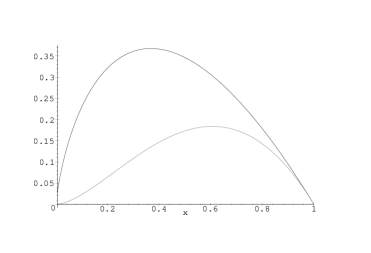
Figure 1: Plot of the dimensionless quantities (upper curve) $(4\pi\nu\sigma_{\max})^{-1}D_{G}(\sigma,t)G_{G}(\sigma,t)$ and (lower curve) $\Gamma_{1}(4\pi\nu\sigma_{\max}^{3})^{-1}D_{G}(\sigma,t)$, both as function of $x\equiv\sigma/\sigma_{\max}$ in the case of a Gaussian monopole.

Fig.1. Plot of the dimensionless quantities (full curve) $(4\pi\nu\sigma_{\max})^{-1}D_{G}(\sigma,t)G_{G}(\sigma,t)$ and (dotted curve) $\Gamma_{1}(4\pi\nu\sigma_{\max}^{3})^{-1}D_{G}(\sigma,t)$, both as function of $x\equiv\sigma/\sigma_{\max}$ in the case of a Gaussian monopole.

2.3 Self-similar decay

In the case of a collection of vortices that evolves self-similarly in time, it is convenient to introduce the dimensionless independent variable $\xi:=(\sigma-\bar{\omega})t$ and the dimensionless functions $\tilde{G}(\xi):=G(\sigma-\bar{\omega},t)/At$ and $\tilde{D}(\xi):=D(\sigma-\bar{\omega},t)/(\sigma-\bar{\omega})^{3}$. When the boundary source term $s(\sigma,t)$ vanishes, as it does in the case of a doubly periodic domain or when the vorticity support remains well separated from the boundary, the self-similar form of (5) is

$$\frac{d\;}{d\xi}\left(\xi\tilde{G}(\xi)\right)=-\frac{d^{2}\;}{d\xi^{2}}\left(\xi^{3}\tilde{D}(\xi)\tilde{G}(\xi)\right),$$

or

$$\xi\tilde{G}(\xi)=-\frac{d\;}{d\xi}\left(\xi^{3}\tilde{D}(\xi)\tilde{G}(\xi)\right)+cte.$$

Assuming that there are no singularities in the vorticity field, one has $G(\sigma,t)\underset{\left|\sigma\right|\rightarrow\infty}{\rightarrow}0$ and it follows then that the constant in the last expression must be zero. Measuring the self-similar density $\tilde{G}(\xi),$ one can solve the last equation for the corresponding diffusion coefficient $\tilde{D}(\xi)$ and get

$$\tilde{D}(\xi)=-\frac{1}{\xi^{3}\tilde{G}(\xi)}\int_{b}^{\xi}ds\,s\tilde{G}(s),$$

where the value of the lower limit of integration $b$ must be chosen according to an appropriate “boundary condition” as illustrated below. If for large $\left|\xi\right|$ the dimensionless vorticity density $\tilde{G}(\xi)$ decays algebraically like $\left|\xi\right|^{-2\alpha}$ (see below) and $2\alpha<3,$ then it follows that the most general decay of $\tilde{D}(\xi)$ is of the form $\left|\xi\right|^{-1}+a\left|\xi\right|^{(2\alpha-3)}$ with $a$ an appropriate constant.

We apply these results to two specific cases: 1) If the self-similar vorticity distribution happens to be Gaussian, i.e., if $\tilde{G}(\xi)=\left(\xi_{o}\sqrt{2\pi}\right)^{-1}\exp\left(-\xi^{2}/2\xi_{o}^{2}\right).$ Then, with $\tilde{D}(\pm\infty)=0$ as “boundary condition” one obtains that $\tilde{D}(\xi)=\xi_{o}^{2}\xi^{-3}$ or, going back to the original quantities, $G(\sigma,t)=At\left(\xi_{o}\sqrt{2\pi}\right)^{-1}\exp\left[-t^{2}(\sigma-\bar{\omega})^{2}/2\xi_{o}^{2}\right]$ and the negative diffusion coefficient is $-D(\sigma,t)=-\xi_{o}^{2}t^{-3}.$ This is the only self-similar case with a $\sigma$-independent $D\left(\sigma,t\right).$ In this case, the time-evolution equation (5) takes a particularly simple form, namely

$$\frac{\partial G(\sigma,t)}{\partial t} =-\xi_{o}^{2}t^{-3}\frac{\partial^{2}G(\sigma,t)}{\partial\sigma^{2}},$$

$$\mathrm{i.e.}\;\frac{\partial G(\sigma,\tau)}{\partial\tau} =+\frac{1}{2}\frac{\partial^{2}G(\sigma,\tau)}{\partial\sigma^{2}}\;\mathrm{with}\;\tau:=\xi_{o}^{2}t^{-2}.$$

In agreement with our findings in IIA, we see that in this case the squared width of the Gaussian distribution decreases in time like $\tau=\xi_{o}^{2}t^{-2}.$
2) The second application is to the self-similar distributions found by Bartello and Warn [[7]] in their simulations performed in a doubly periodic domain of size $A$. Qualitatively speaking, their results can be summarized by the following expression

$$\tilde{G}_{s}(\xi) =c\left(\xi_{o}^{2}+\xi^{2}\right)^{-\alpha},\;\left|\xi\right|\leq\xi_{M}$$ (7)

$$\tilde{G}_{s}(\xi) =0,\;\left|\xi\right|>\xi_{M}.$$

with $\xi_{o}\simeq 10,$ $\alpha\simeq 0.7$ and $\xi_{M}$ growing approximately like $\sqrt{t}$, from 200 to 500. The value of $c$ being such that $\int\!d\xi\,\tilde{G}(\xi)=1.$ Vorticity values such that $\left|\sigma\right|t<\xi_{o}$ are associated mainly with thin filaments in the background “sea” while those such that $\left|\sigma\right|t>\xi_{o}$ correspond to the localized vortices. At the positions with the largest vorticity value the gradient $\nabla\omega$ vanishes, therefore, it is natural to take as “boundary condition” $\tilde{D}_{s}(\xi_{M})=0.$ One gets then the following effective diffusion coefficient in vorticity-space

$$\tilde{D}_{s}(\xi)=\frac{\left(\xi_{o}^{2}+\xi^{2}\right)^{\alpha}}{2(1-\alpha)\left|\xi\right|^{3}}\left[\left(\xi_{o}^{2}+\xi_{M}^{2}\right)^{\left(1-\alpha\right)}-\left(\xi_{o}^{2}+\xi^{2}\right)^{(1-\alpha)}\right],\;\left|\xi\right|\leq\xi_{M}(t).$$

Going back to the original variables, this effective diffusion coefficient reads,

$$D_{s}(\sigma,t)=\frac{\left(\xi_{o}^{2}+\sigma^{2}t^{2}\right)^{\alpha}}{2(1-\alpha)t^{3}}\left[\left(\xi_{o}^{2}+\xi_{M}^{2}\right)^{\left(1-\alpha\right)}-\left(\xi_{o}^{2}+\sigma^{2}t^{2}\right)^{(1-\alpha)}\right],\quad\left|\sigma\right|t\leq\xi_{M}(t).$$

The average of $\left|\nabla\omega\right|^{2}$ in the thin filaments is not zero so that at $\sigma=0$ we have

$$D_{s}(0,t)=\frac{\xi_{o}^{2}}{2(1-\alpha)t^{3}}\left[\left(1+\frac{\xi_{M}^{2}}{\xi_{o}^{2}}\right)^{\left(1-\alpha\right)}-1\right]\simeq\frac{\xi_{o}^{2\alpha}\xi_{M}^{2\left(1-\alpha\right)}}{2(1-\alpha)t^{3}}.$$

The origin, $\sigma=0$ is a local minimum of $D_{s}(\sigma,t),$ moreover there is one maximum, namely

$$\max D(\sigma,t)=\alpha^{\frac{\alpha}{1-\alpha}}\frac{\xi_{o}^{2}+\xi_{M}^{2}(t)}{2t^{3}}\quad at\quad\sigma^{\ast}t=\sqrt{\alpha^{\frac{\alpha}{1-\alpha}}\left(\xi_{o}^{2}+\xi_{M}^{2}(t)\right)-\xi_{o}^{2}}\simeq\alpha^{\frac{\alpha}{2(1-\alpha)}}\xi_{M}.$$

For large $t,$ the maximum decays like $t^{-2}$ while $D(0,t)$ decays faster, namely like $t^{-(2+\alpha)}.$
In Fig.2, we plot the dimensionless quantities $t^{3}D_{s}(\sigma,t)\xi_{M}^{-2}$ and $4\left(cA\xi_{M}^{2(1-\alpha)}\xi_{o}^{2\alpha}\right)^{-1}t^{2}D_{s}(\sigma,t)G_{s}(\sigma,t)$ as functions of $x\equiv\sigma t/\xi_{M}$.

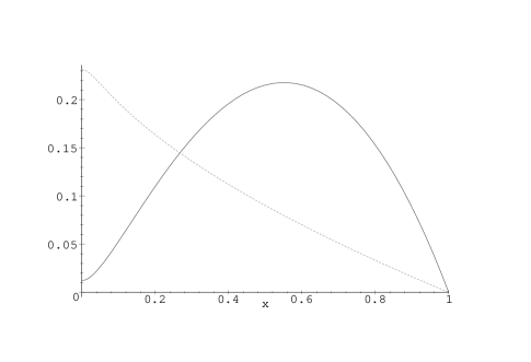
Figure 2: Plot of the dimensionless quantities (full curve) $t^{3}D_{s}(\sigma,t)\xi_{M}^{-2}$ and (dotted curve) $4\left(cA\xi_{M}^{2(1-\alpha)}\xi_{o}^{2\alpha}\right)^{-1}t^{2}D_{s}(\sigma,t)G_{s}(\sigma,t)$ as functions of $x\equiv\sigma t/\xi_{M}$ in the case of self-similar decay with $\xi_{o}=10$ and for $\xi_{M}=300$, as discussed in the main text.

3 The changes in the vorticity-area distribution

3.1 General considerations

In comparison to the case of a passive scalar, the spatial distribution of vorticity does not play such a central role as one realizes from Arnold’s observation that the stationary solutions of the Euler equations in two dimensions correspond to energy extrema under the constraint of fixed vorticity areas [[15] ,[16]]. Arnold’s observation says then that the stationary solutions of the 2D Euler equations, $\omega_{S}(x,y),$ are the states with extremal values of the energy compatible with the vorticity-area density

$$G_{S}(\sigma):=\int\!dxdy\,\delta(\sigma-\omega_{S}(x,y)).$$

Therefore, the vorticity-area density $G_{S}(\sigma)$ of a QSS (and the geometry of the domain) determine $\omega_{S}(x,y),$ the spatial distribution of vorticity in the coherent structure. From this we conclude that when studying the process leading to the QSS in viscous fluids, special attention should be paid to the differences between the initial vorticity-area density $G(\sigma,0)$ and $G_{S}(\sigma),$ the one in the QSS. A convenient way of studying these changes would be through the differences in the moments of these distributions, which will be denoted by $\Delta_{n},$ i.e.,

$$\Delta_{n} :=\Gamma_{n}^{o}-\Gamma_{n}^{S},\;\mathrm{with}$$

$$\Gamma_{n}^{o} :=\int\!dxdy\,\omega^{n}(x,y,0)=\int\!d\sigma\,\sigma^{n}G(\sigma,0)\;\mathrm{and}$$

$$\Gamma_{n}^{S} :=\int\!dxdy\,\omega_{S}^{n}(x,y)=\int\!d\sigma\,\sigma^{n}G_{S}(\sigma).$$

The dimensionless ratios $\Delta_{n}/\Gamma_{n}^{S}$ would offer a good characterization of the changes experienced by the vorticity-area distribution. In the next Subsections we present another possibility, linked to the predictions of a QSS according to a statistical-mechanics approach, which is constructed from an $\omega_{S}(\psi_{S})$ relation measured either in experiments or in numerical simulations.

3.2 The changes in the moments according to the statistical mechanics approach

It is proven in the Appendix that when the quasi-stationary vorticity field $\omega_{S}(x,y)$ and the initial field $\omega(x,y,0)$ are related as predicted by the statistical mechanical theory then the observed $\Delta_{n}$ take the values $\delta_{n}$

$$\delta_{n} =\int\!dxdy\,i_{n}(\psi),$$ (8)

$$\mathrm{with}\;i_{1} :=0\;\mathrm{and}$$

$$i_{n+1}(\psi) =\left[\Omega(\psi)-\frac{1}{\beta}\frac{d\;}{d\psi}\right]i_{n}(\psi)+\left(-\beta\right)^{-1}\frac{d\Omega^{n}}{d\psi}.$$

defined in terms of the associted$\ \Omega(\psi)$ relation and an inverse temperature $\beta.$ In particular, for $n\leq 4,$ we have

$$\delta_{1} =0,$$ (9)

$$\delta_{2} =-\beta^{-1}\int\!dxdy\,(d\Omega/d\psi),$$

$$\delta_{3} =\beta^{-2}\int\!dxdy\left[\frac{d^{2}\Omega}{d\psi^{2}}-3\beta\Omega\frac{d\Omega}{d\psi}\right],$$

$$\delta_{4} =-\beta^{-3}\int\!dxdy\,\left[\frac{d^{3}\Omega}{d\psi^{3}}-4\beta\Omega\frac{d^{2}\Omega}{d\psi^{2}}+6\beta^{2}\Omega^{2}\frac{d\Omega}{d\psi}-3\beta\left(\frac{d\Omega}{d\psi}\right)^{2}\right].$$

In the next Subsection we propose the use of $\delta_{n}$ as yardsticks in order to quantify the departure of the observed changes $\Delta_{n}$ from the theoretical predictions.

3.3 Analysis of experimental results

In many cases, the predictions obtained from different theories are not very different and it is not obvious which prediction agrees better with the experimental data, see, e.g., [[17] ,[24]] . Therefore, it is important to develop objective, quantitative measures of such an agreement.

The results of the previous Subsection lead us to conclude that there is useful information encoded in the functional dependence of $\omega_{S}(\psi_{S})$ and that this information can be used for the quantification of the vorticity redistribution process in any experiment or numerical simulation, i.e., also when (13) and (14) do not necessarily hold, as long as there is no leakage and creation or destruction of vorticity at the boundary is negligeable. We propose that one should proceed as follows:
1) Identify the predicted$\ \Omega(\psi)$ relation of the preceeding Subsection and the Appendix with the $\omega_{S}(x,y)\approx\omega_{S}(\psi_{S})$ of the observed QSS; usually, this satisfies $d\omega_{S}/d\psi_{S}\neq 0,$
2) Determine an effective value of $\beta$ from $\Delta_{2},$ the measured change in the second moment of the vorticity-area distribution and from the measured $\omega_{S}(\psi_{S})\$relation by, confer the second line of (9),

$$\beta:=-\frac{\int\!dxdy\,(d\omega_{S}/d\psi_{S})}{\Delta_{2}}.$$ (10)

Since $\Delta_{2}\geq 0,$ the sign of $\beta$ is always opposite to that of $d\omega_{S}/d\psi_{S}.$
3) Using this value of $\beta$ compute from equation (8), with $\Omega(\psi)$ replaced by $\omega_{S}(\psi_{S}),$ the values of the yardsticks $\delta_{n}$ for $n\geq 3.$
4) The measured changes in the third and higher moments, $\Delta_{n}$ with $n\geq 3,$ should be quantified by the dimensionless numbers $\alpha_{n}:=\Delta_{n}/\delta_{n}.$ These numbers are all equal to 1 if and only if the QSS agrees with the statistical mechanical prediction corresponding to the initial distribution $G(\sigma,0)$ with equal initial and final energies,

$$\omega_{S}(\psi_{S})\;\mathrm{corresponds\;to\;a\;statitistical\;equilibrium}\leftrightarrow\alpha_{3}=\cdots=\alpha_{n}=\cdots=1.$$ (11)

It is for this reason that one should prefer these dimensionless quantities to other ones like, e.g., $\Delta_{n}/\Gamma_{n}^{S}$.

In closing, it may be worthwhile recalling that, at least in some cases, the agreement between an experiment and the statistical mechanical prediction can be greatly improved by taking as “initial condition” not the field at the start of the experiment but a later one, after some preliminary mixing has taken place but well before the QSS appears, see [ [25]]. This improvement can be quantified by measuring the convergence of the corresponding $\alpha_{n}=\Delta_{n}/\delta_{n}$ towards 1. In other cases, a detailed consideration of the boundary is necessary and, sometimes, the satistical mechanics approach may be applicable in a well-chosen subdomain, see [[26] ,[24]].

3.4 Examples

A possible $\Omega(\psi)$ relation resulting from the statistical mechanical theory that may be compared successfully to many experimentally found curves is

$$\Omega_{t}(\psi)=\Omega_{o}\frac{\sinh\chi\psi}{B+C\cosh\chi\psi},$$ (12)

with appropriately chosen constants $\Omega_{o},B,C$ and $\chi.$ In particular, the flattening in the scatter plots observed in [[27]] can be fitted by this expression while the case $C=0,$ corresponds to the identical point-vortices model [[28] ,[29]] and the case $\chi\rightarrow 0$ with $\chi\Omega_{o}/(B+C)\rightarrow$finite, corresponds to a linear scatter-plot. In all these cases, the $\delta_{n}$ can be derived, as explained in the Appendix, by means of a cumulant generating function, confer (17),

$$\kappa_{t}(\lambda,\psi) =-\beta\Omega_{o}\int^{\lambda}\frac{\sinh\chi\left(\psi+\xi\right)}{B+C\cosh\chi\left(\psi+\xi\right)}d\xi$$

$$=-\frac{\beta\Omega_{o}}{\chi C}\ln\frac{B+C\cosh\chi\left(\psi+\lambda\right)}{B+C\cosh\chi\psi}.$$

Expanding this in powers of $\lambda$ leads to the cumulants of the microscopic vorticity distribution. In particular,

$$\left\langle\sigma^{2}\right\rangle_{t}-\Omega_{t}^{2} =-\beta^{-1}\frac{d\Omega_{t}}{d\psi}$$

$$=-\frac{\chi\Omega_{o}}{\beta}\frac{B\cosh\chi\psi+C}{\left(B+C\cosh\chi\psi\right)^{2}}.$$

Integrating this over the area, one obtains that

$$\Delta_{2}^{t}=-\frac{\chi\Omega_{o}}{\beta}\int\!dxdy\,\frac{B\cosh\chi\psi+C}{\left(B+C\cosh\chi\psi\right)^{2}}.$$

Knowledge of $\Delta_{2}^{t}$ and of $\Omega_{t}(\psi)$ allows us to determine the value of $\beta.$ Once $\beta$ has been fixed, one can apply (8) and (11) in order to quantify the higher-order moments $\Delta_{n}$ and in so doing to estimate the validity of equation (12) as the prediction from the statistical-mechanics approach.

If the scatter-plot is linear, $\Omega(\psi)=k\psi,$ then (17) tells us that

$$\kappa_{linear}(\lambda,\psi)=-\beta k\left[\lambda\psi+\frac{1}{2}\lambda^{2}\right].$$

This implies a simple relation between the initial vorticity-area distribution $G(\sigma,0)$ and $G_{S}(\sigma),$ the distribution in the QSS, namely

$$\int\!d\sigma\,\exp(-\lambda\beta\sigma)G\left(\sigma,0\right)=\exp(\frac{1}{2}\lambda^{2}\beta k)\int\!d\sigma\,\exp(-\lambda\beta\sigma)G_{S}\left(\sigma\right).$$

Recall that, as already indicated immediately after (10), $\beta k\leq 0.$ Assuming that the Laplace transformation can be inverted, we get for the linear case $\Omega(\psi)=k\psi,$ that

$$G\left(\sigma,0\right)=\int\!d\tau\,\exp(-\frac{\left(\sigma-\tau\right)^{2}}{2\left|\beta k\right|})G_{S}\left(\tau\right)$$

In particular, if the QSS has a Gaussian vorticity-area density with a variance equal to $\Sigma^{2}$ and the predictions of the statistical mechanical approach hold, then the initial distribution $G\left(\sigma,0\right)$ must also be a Gaussian with variance equal to $\left(\Sigma^{2}-\beta k\right)\geq\Sigma^{2},$ in agreement with the results in [ [19] ,[30]]. Notice that knowing $G(\sigma,0)$ and the energy of the initial state is not enough in order to determine the spatial dependence of the initial vorticity field $\omega(x,y,0)$.

4 Conclusions

In this paper, the object at the center of our attention has been the vorticity-area density $G(\sigma,t)$ and its time evolution in two-dimensional, viscous flows. In Section 2 we have shown that this density evolves according to an advection-diffusion equation, equation (5), with a time dependent, negative diffusion coefficient. If vorticity is destroyed or created at the domain boundaries then the evolution equation contains also a source term. The equation is exact: it follows from the Navier-Stokes equation with no approximations made. For the purpose of illustration, explicit calculations have been presented for the case of a Gaussian monopole in 22.1 and for the case of self-similar decay in 22.3. We think that it will be instructive to apply these ideas to the analysis of data that is available from numerical simulations and laboratory experiments. In fact, it should be possible to determine this effective diffusion coefficient $D(\sigma,t)$ on the basis of such data. Then it would be of interest to establish a quantitative classification of the QSS formation processes, e.g., by considering the various possible behaviours of this coefficient and, in particular, confer Figs. 1 and 2, of $G(\sigma,t)D(\sigma,t)$. In the case of self-similar decay, one could attempt a closure approximation in order to predict the effective diffusion coefficient like it is done, for very similar quantities, in the theory of passive-scalar dispersion by random velocity fields, e.g., Kraichnan’s linear Ansatz [[23]].
In Section 3 we considered the changes in $G(\sigma,t)$ when starting from an arbitrary vorticity field and ending at a high-Reynolds’ number, quasi-stationary state characterized by an $\omega_{S}(\psi_{S})$ relation. In 33.2 and in the Appendix, we showed how to generate from such an $\omega$-$\psi$ plot an infinite set of moments $\delta_{n}$, confer (8). The changes $\Delta_{n}$ in the moments of the vorticity distribution that are observed in a numerical simulation or in the laboratory equal these $\delta_{n}$ if and only if the initial and final distributions are related to each other in the way predicted by the statistical mechanical approach. Therefore, these changes in the vorticity distribution moments can be quantified in terms of the dimensionless ratios $\Delta_{n}/\delta_{n}.$ The deviations of the ratios $\Delta_{n}/\delta_{n}$ from the value 1 as determined on the basis of the data gives a direct way of quantifying the validity of the statistical-mechanics approach. In 33.3 we discussed how to apply this to experimental measurements provided that the leakage or creation and destruction of vorticity at the boundaries is negligeable. Finally, in Subsection 33.4, we considered two relevant $\omega$-$\psi$ relations: a linear one and a much more general one, given by equation (12). Many of these ideas should be applicable also to more realistic systems, e.g., when potential vorticity is a Lagrangian invariant.

Acknowledgements: We have benefitted from numerous discussions with H. Brands, from P.-H. Chavanis’ comments and from the comments of the referees. The interest shown by H. Clercx, G.-J. van Heijst, S. Maassen and J.J. Rasmussen has been most stimulating.

5 Appendix

We prove now that if and only if the QSS happens to coincide with the prediction of the statistical mechanical approach, then the changes in the moments $\Delta_{n}$ take the values $\delta_{n}$ as defined in (8).
Recall that in the statistical mechanical approach one identifies $\omega_{S}(x,y),$ the vorticity of the QSS, with $\left\langle\sigma\right\rangle:=\int\!d\sigma\,\sigma\rho(\sigma,\psi),$ the average value of the microscopic vorticity $\sigma$ with respect to a vorticity distribution $\rho(\sigma,\psi)$ which is given by

$$\rho(\sigma,\psi) :=Z^{-1}\exp\left[-\beta\sigma\psi(x,y)+\mu(\sigma)\right],$$ (13)

$$\mathrm{with\;}Z(\psi) :=\int\!d\sigma\,\exp\left[-\beta\sigma\psi+\mu(\sigma)\right]$$

$$\mathrm{and\;define\;}\Omega(\psi) :=\left\langle\sigma\right\rangle=\int\!d\sigma\,\sigma\rho(\sigma,\psi).$$

In (13), $\beta$ and $\mu(\sigma)$ are Lagrange multipliers such that the energy per unit mass and the microscopic-vorticity area distribution $g(\sigma):=\int\!dxdy\,\rho(\sigma,\psi(x,y))$ have the same values as in the initial distribution, i.e., $g(\sigma)=G(\sigma,0)$. Consequently, the spatially integrated moments are given by

$$\int\!dxdy\,\left\langle\sigma^{n}\right\rangle =\int\!d\sigma\,\sigma^{n}g(\sigma)=\int\!d\sigma\,\sigma^{n}G(\sigma,0)=\Gamma_{n}^{o}$$ (14)

$$\mathrm{while\;}\Gamma_{n}^{S} =\int\!dxdy\,\Omega^{n}(\psi)=\int\!dxdy\,\left\langle\sigma\right\rangle^{n}.$$

Denote by $\delta_{n}$ the predicted change in the $n$-th moment, i.e.,

$$\delta_{n}=\int\!dxdy\,\left[\left\langle\sigma^{n}\right\rangle-\left\langle\sigma\right\rangle^{n}\right]=:\int\!dxdy\,i_{n}.$$ (15)

To the probability distribution $\rho(\sigma,\psi),$ defined in (13), we associate a cumulant generating function

$$\kappa(\lambda,\psi):=\ln\left\langle\exp\left(-\lambda\beta\sigma\right)\right\rangle.$$ (16)

This satisfies

$$\frac{\partial\kappa(\lambda,\psi)}{\partial\lambda}=-\beta\Omega(\psi+\lambda)\,,$$ (17)

as it can be shown by first noticing that

$$\left\langle\exp\left(-\lambda\beta\sigma\right)\right\rangle=\frac{Z(\psi+\lambda)}{Z(\psi)}$$

so that $\kappa(\lambda,\psi)=\ln Z(\psi+\lambda)-\ln Z(\psi)$ and then using $\int\!d\sigma\,\sigma\rho(\sigma,\psi+\lambda)=\Omega(\psi+\lambda)$ for the computation of $\partial\kappa/\partial\lambda$. Expanding both sides of (17) in powers of $\lambda$, it follows that $\kappa_{n}(\psi),$ the $n$-th local cumulant of $-\beta\sigma,$ is related to $\Omega(\psi)$ by

$$\kappa_{n}(\psi)=-\beta\frac{d^{n-1}}{d\psi^{n-1}}\Omega(\psi).$$ (18)

For example, for $1\leq n\leq 4,$ these equalities read

$$\beta\left\langle\sigma\right\rangle =\beta\Omega,$$

$$\beta^{2}\left[\left\langle\sigma^{2}\right\rangle-\Omega^{2}\right] =-\beta\frac{d\Omega}{d\psi},$$

$$\beta^{3}\left[\left\langle\sigma^{3}\right\rangle-3\Omega\left\langle\sigma^{2}\right\rangle+2\Omega^{3}\right] =\beta\frac{d^{2}\Omega}{d\psi^{2}},$$

$$\beta^{4}\left[\left\langle\sigma^{4}\right\rangle-3\left\langle\sigma^{2}\right\rangle^{2}-4\left\langle\sigma^{3}\right\rangle\Omega+12\left\langle\sigma^{2}\right\rangle\Omega^{2}-\Omega^{4}\right] =-\beta\frac{d^{3}\Omega}{d\psi^{3}}.$$

For our purposes, it is essential to eliminate from these equations products like $\Omega\left\langle\sigma^{2}\right\rangle$ and $\left\langle\sigma^{2}\right\rangle^{2}$ because their integrals over the whole domain cannot be related to known quantities. In fact, the differences $\delta_{n}$ can be directly expressed in terms of $\Omega(\psi)$ and its derivatives, i.e., in terms of known quantities, as we now show. To this end, one considers first the generating function of the local moment differences $i_{n}$, which will be denoted by $i(\lambda,\psi).$ One has that, confer (15),

$$i(\lambda,\psi):=\left\langle\exp\left(-\lambda\beta\sigma\right)\right\rangle-\exp\left(-\lambda\beta\left\langle\sigma\right\rangle\right),$$

This is related to the cumulants generating function $\kappa(\lambda,\psi),$ confer equation (16), by

$$\kappa(\lambda,\psi)=\ln\left[i(\lambda,\psi)+\exp\left(-\lambda\beta\left\langle\sigma\right\rangle\right)\right].$$

Expanding both sides of this identity in powers of $\lambda$ and making use of (18), one obtains the recursive expressions for the $i_{n}(\psi)$ given in equation (8); integrating these over the area $A,$ one finally gets the results stated in 33.2.

References

- [1] J.C. McWilliams, “The emergence of isolated coherent vortices in turbulent flow”, J. Fluid Mech. 146, 21 (1984).
- [2] P. Santangelo, R. Benzi, B. Legras, “The generation of vortices in high-resolution, two-dimensional decaying turbulence and the influence of initial conditions on the breaking of self similarity”, Phys. Fluids A 1, 1027 (1989).
- [3] G.F. Carnevale, J.C. McWilliams, Y. Pomeau, J.B. Weiss and W.R. Young, “Evolution of vortex statistics in two-dimensional turbulence”, Phys.Rev.Letters 66, 2735 (1991).
- [4] G.F. Carnevale, J.C. McWilliams, Y. Pomeau, J.B. Weiss and W.R. Young, “Rates, pathways, and end states of nonlinear evolution in decaying two-dimensional turbulence: Sacling theory versus selective decay”, Phys.Fluids A 4, 1314 (1992).
- [5] O. Cardoso, D. Marteau and P. Tabeling, “Quantitative experimental study of the free decay of quasi-two-dimensional turbulence”, Phys. Rev. E 49, 454 (1994).
- [6] V. Borue, “Inverse energy cascade in stationary two-dimensional homogeneous turbulence”, Phys.Rev.Letters 72, 1475 (1994).
- [7] P. Bartello and T. Warn, “Self-similarity of decaying two-dimensional turbulence”, J. Fluid Mechanics 326, 357–372 (1996).
- [8] G.J.F. van Heijst and J.B. Flór, “Dipole formations and collisions in a stratified fluid”, Nature 340, 212 (1989).
- [9] D. Marteau, O. Cardoso, and P. Tabeling, “Equilibrium states of 2D turbulence: an experimental study”. Phys. Rev. E 51, 5124-5127 (1995).
- [10] E. Segre and S. Kida, “Late states of incompressible 2D decaying vorticity fields”, Fluid Dyn. Res. 23, 89 (1998).
- [11] H. Brands; private communication.
- [12] E.J. Hopfinger and G.J.F. van Heijst, “Vortices in Rotating Fluids”, Ann.Rev.Fluid Mech. 25, 2041 (1993).
- [13] R.H. Kraichnan and D. Montgomery, “Two dimensional turbulence”, Rep. Prog. Phys. 43, 547 (1980).
- [14] P.-H. Chavanis, J. Sommeria and R. Robert, “Statistical mechanics of two-dimensional vortices and collisionless stellar systems”, Astrophys. J. 471 385–399 (1996).
- [15] V.I. Arnold 1966, Izv. Vyssh. Uchebn. Zaved. Mathematica 54 (5), 3-5, “On an a priori estimate in the theory of hydrodynamical stability”. English translation in: 1969, American Math. Soc. Transl., Series 2, 79, 267-269.
- [16] V.I. Arnold, 1978 Appendix 2 of Mathematical Methods of Classical Mechanics,.Springer Verlag, 462 pp. Russian original by Nauka, 1974.
- [17] A. Majda and M. Holen, “Dissipation, topography and statistical theories for large scale coherent structures ”, Comm. Pure and Appl. Math. L 1183–1234 (1997); M. Grote and A. Majda, “Crude closure dynamics through large scale statistical theories”, Phys. Fluids 9, 3431–3442 (1997).
- [18] J. Miller, “Statistical mechanics of Euler’s equation in two dimensions”, Phys. Rev. Lett. 65, 2137 (1990).
- [19] J. Miller, P.B. Weichman, and M.C. Cross, “Statistical mechanics, Euler’s equation, and Jupiter’s Red Spot”, Phys. Rev. A 45, 2328 (1992).
- [20] R. Robert, “Etat d’équilibre statistique pour l’écoulement bidimensionnel d’un fluide parfait, C.R. Acad.Sci. Paris t 311 (Série I), 575 (1990).
- [21] R. Robert, “Maximum entropy principle for two-dimensional Euler equations”, J. Stat. Phys. 65, 531 (1991).
- [22] R. Robert and J. Sommeria, “Statistical equilibrium states for two dimensional flows”, J. Fluid Mech. 229, 291 (1991).
- [23] R.H. Kraichnan, Physical Review Letters 72 1016 (1994), 75 240 (1995) and 78 4922 (1997).
- [24] H. Brands, P.-H. Chavanis, R.A. Pasmanter and J. Sommeria, “Maximum entropy versus minimum enstrophy vortices”, Phys. of Fluids 11, 3465–3477 (1999).
- [25] H. Brands, J. Stulemeyer, R.A. Pasmanter and T.J. Schep, “A mean field prediction of the asymptotic state of decaying 2D turbulence”, Phys. Fluids 9, 2815-2817 (1998).
- [26] P.-H. Chavanis and J. Sommeria, “Classification of robust isolated vortices in two-dimensional turbulence”, J. Fluid Mechanics 356 259–296 (1998).
- [27] A.H. Nielsen, J.J. Rasmussen and M.R. Schmidt, “Self-organization and coherent structures in plasmas and fluids”, Phys. Scr. T63, 49–58 (1996) ; A.H. Nielsen and J.J. Rasmussen, “Formation and evolution of a Lamb dipole”, Phys. Fluids 9, 982–991 (1997).
- [28] D. Montgomery, W. Matthaeus, W. Stribling, D. Martinez, and S. Oughton, “Relaxation in two dimensions and the sinh-Poisson equation”, Phys. Fluids A 4, 3 (1992).
- [29] D. Montgomery, X. Shan, and W. Matthaeus, “Navier-Stokes relaxation to sinh-Poisson states at finite Reynolds numbers”, Phys. Fluids A 5, 2207 (1993).
- [30] H. Brands, Two-dimensional Coherent Structures and Statistical Mechanics, Ph.D. Thesis, University of Amsterdam (1998).