J.Stat.Phys, submitted. Version of
  
Dynamics of Finger Formation in Laplacian Growth without Surface Tension

Abstract

We study the dynamics of “finger” formation in Laplacian growth without surface tension in a channel geometry (the Saffman-Taylor problem). Carefully determining the role of boundary geometry (resulting in reflection symmetry, not periodicity), we construct field equations of motion, these central to the analytic power we can here exercise. Initially we consider an explicit analytic class of maps to the physical space, a basis of solutions for infinite fluid in an infinitely long channel, characterized by meromorphic derivatives. We dynamically verify that these maps never lose analyticity in the course of temporal evolution, thus justifying the underlying machinery. However, the great bulk of these solutions can lose conformality in time, this the circumstance of finite-time singularities. By considerations of the nature of the analyticity of all these solutions, we do, however, show that those free of such singularities inevitably result in a single asymptotic “finger”. This is purely nonlinear behavior: the very early “finger” actually already has a waist, this having signalled the end of any linear regime. The single “finger” has nevertheless an arbitrary width determined by initial conditions. This is in contradiction with the experimental results that indicate selection of a finger of width 1/2. In the last part of this paper we motivate that such a solution can be determined by the boundary conditions when the fluid is finite. This is a strong signal that finiteness is determinative of pattern selection.

1 Introduction

The aim of this paper is to offer some careful analysis of the initial value problem associated with Laplacian growth without surface tension in an infinite channel geometry. It is well known for quite some time that this problem possesses asymptotic solutions in the form of a “finger” whose width $\lambda$ may be taken apparently arbitrarily [1]. In experiments which are performed in a finite channel and in which the effective surface tension is very small a single width ($\lambda=1/2$) is selected[1, 2]. Previous work explained how a unique steady solution is selected by the existence of surface tension [3, 4, 5, 6]. That work never explored the question how this solution arises from arbitrary initial conditions.

Here we consider the initial value problem, and explain how a very wide class of initial conditions ends up with an asymptotic solution of an interface in the form of a single finger. Our initial conditions may include very complicated interfaces, indeed having many features. It is important to understand the generic dynamical mechanism that is responsible for the generation of a single finger that becomes an asymptotic solution. We show that in the infinite channel the width of the finger is not selected (notwithstanding some recent claims to the contrary [7]).

We next remark that the experiments in which selection is observed include, in addition to surface tension, also a second boundary condition. One can set up the experiment in various ways, like ending the material fluid at atmospheric pressure, or connect it to a pump that sustains the flow. We discuss the various boundary conditions that can be imposed on the second boundary, and show that some natural choices impose a unique solution with width 1/2. This discussion serves as an introduction to a substantial treatment of finiteness in a forthcoming paper [8]

The structure of the paper is as follows: in Sect.2 we recall the analytic theory of Laplacian growth in channel geometry. The novel aspect of our treatment is the introduction of the equation of motion for the conformal map that explicitly takes into account reflection symmetry of the solutions in the complex plane. The significant virtue of our method is that it totally obviates any need for Hilbert transforms and so forth that are required in the usual, pure boundary treatment. .In Sect.3 we show that analytic initial data remain analytic for all available time. On the contrary, conformality can be lost in finite time, and in Sect.5 we discuss how this may happen in generic situations, and discuss how a regulation, such as surface tension, accomplishes the cure of this disease. In Sect.4 we come to understand that any generic initial condition has a single Saffman-Taylor finger asymptotics. In Sect.6 we discuss finite boundary conditions. We observe that the imposition of a downstream boundary condition may uniquely select a solution of width 1/2. In Sect.7 we offer a summary and a discussion.

2 Analytic solutions of Laplacian Growth in Channel Geometry

A The physical problem and the mathematical formulation

We are interested in the so-called Saffman-Taylor problem of determining the motion of an interface $\gamma(t)$ between two fluids of different viscosities in a Hele-Shaw cell. We can think of air displacing oil as a standard example [9]. The cell is a channel made of two long rectangular plates displaced by a small distance $b$. We chose $x$ to denote the long lateral coordinate, whereas $y$ denotes the transversal direction of the cell, $0\leq y\leq\pi$ in suitable units, (see Fig.1a). When the gap $b$ is considerably smaller than the lateral width of the cell, and non-slip boundary conditions are taken at the upper and lower plates, then the velocity field $\textstyle v$ in the driven fluid satisfies Darcy’s law

$${\mathchoice{{\hbox{\boldmath$\displaystyle v$}}}{{\hbox{\boldmath$\textstyle v$}}}{{\hbox{\boldmath$\scriptstyle v$}}}{{\hbox{\boldmath$\scriptscriptstyle v$}}}}={-b^{2}\over 12\mu}{\mathchoice{{\hbox{\boldmath$\displaystyle\nabla$}}}{{\hbox{\boldmath$\textstyle\nabla$}}}{{\hbox{\boldmath$\scriptstyle\nabla$}}}{{\hbox{\boldmath$\scriptscriptstyle\nabla$}}}}p\ ,$$ (1)

where $p$ is the pressure field and $\mu$ the viscosity. Because of the assumed very small viscosity of the driving fluid, its pressure is almost constant (taken to be zero), while in the driven fluid, by virtue of incompressibility, ${\mathchoice{{\hbox{\boldmath$\displaystyle\nabla$}}}{{\hbox{\boldmath$\textstyle\nabla$}}}{{\hbox{\boldmath$\scriptstyle\nabla$}}}{{\hbox{\boldmath$\scriptscriptstyle\nabla$}}}}\cdot{\mathchoice{{\hbox{\boldmath$\displaystyle v$}}}{{\hbox{\boldmath$\textstyle v$}}}{{\hbox{\boldmath$\scriptstyle v$}}}{{\hbox{\boldmath$\scriptscriptstyle v$}}}}=0$, the pressure is harmonic:

$$\Delta p=0\ .$$ (2)

The boundary conditions on the interface are determined by first requiring the non-penetrability of the two fluids in contact. This means an equality of the normal velocity of the interface ${\mathchoice{{\hbox{\boldmath$\displaystyle v$}}}{{\hbox{\boldmath$\textstyle v$}}}{{\hbox{\boldmath$\scriptstyle v$}}}{{\hbox{\boldmath$\scriptscriptstyle v$}}}}_{i}\cdot{\mathchoice{{\hbox{\boldmath$\displaystyle n$}}}{{\hbox{\boldmath$\textstyle n$}}}{{\hbox{\boldmath$\scriptstyle n$}}}{{\hbox{\boldmath$\scriptscriptstyle n$}}}}$ and of the normal velocity of the fluid at the interface. Secondly, the pressure of the fluid at the interface is given by the relation

$$p_{air}-p=\sigma\kappa\ ,$$ (3)

where $\sigma$ and $\kappa$ are interfacial surface tension and curvature respectively. On the lateral walls ($y=0,\pi$) the normal velocity of the fluid vanishes, and as $x\to\infty$, far ahead of the interface, the flow is taken as uniform, parallel to the $x$ axis, and of magnitude $V$. Here we take $\sigma=0$. The boundary condition (3) now simplifies to taking constant pressure on the interface:

$$p=0~{}{\rm at~{}the~{}interface~{}\gamma(t)};~{}\sigma=0\ .$$ (4)

In consequence of Eq.(1) we also need to require that the normal derivative of the pressure vanishes at the lateral walls. This means that the interface must be normal to the two lateral walls. As the flow is approximately two-dimensional and obeys Laplace’s equation, in the usual fashion one produces an analytic function $\tilde{h}^{\prime}(z)$,

$$\tilde{h}^{\prime}(z)=-\partial_{x}p+i\partial_{y}p=v_{x}-iv_{y}\equiv\bar{\mathchoice{{\hbox{\boldmath$\displaystyle v$}}}{{\hbox{\boldmath$\textstyle v$}}}{{\hbox{\boldmath$\scriptstyle v$}}}{{\hbox{\boldmath$\scriptscriptstyle v$}}}}\ ,$$ (5)

where $z=x+iy$. (With $\Delta p=0$, $\tilde{h}^{\prime}(z)$ satisfies the Cauchy-Riemann conditions.) The integral of $\tilde{h}^{\prime}(z)$ is

$$\tilde{h}(z)=-p(z)+is(z)\ ,$$ (6)

with $s(z)$ the harmonic function conjugate to $-p(z)$. The function $s(z)$ is typically multivalued. Consider now an arbitrary curve $\gamma$, and denote by $\Phi_{\gamma}(t)$ the time dependent flux that crosses $\gamma$. It is convenient to consider $V_{\gamma}(t)$, the mean channel velocity, by dividing $\Phi$ by the constant channel width $\pi$. With $\hat{n}$ denoting the right-handed normal

$$V_{\gamma}(t)=\frac{1}{\pi}\int_{\gamma}v_{n}d\ell\ ,$$ (7)

where $d\ell$ is an arc-length differential. Denoting $\hat{\mathchoice{{\hbox{\boldmath$\displaystyle u$}}}{{\hbox{\boldmath$\textstyle u$}}}{{\hbox{\boldmath$\scriptstyle u$}}}{{\hbox{\boldmath$\scriptscriptstyle u$}}}}$ the unit vector orthogonal to the plane we can write

$$v_{n}d\ell = {\mathchoice{{\hbox{\boldmath$\displaystyle v$}}}{{\hbox{\boldmath$\textstyle v$}}}{{\hbox{\boldmath$\scriptstyle v$}}}{{\hbox{\boldmath$\scriptscriptstyle v$}}}}\cdot(d{\mathchoice{{\hbox{\boldmath$\displaystyle\ell$}}}{{\hbox{\boldmath$\textstyle\ell$}}}{{\hbox{\boldmath$\scriptstyle\ell$}}}{{\hbox{\boldmath$\scriptscriptstyle\ell$}}}}\times\hat{\mathchoice{{\hbox{\boldmath$\displaystyle u$}}}{{\hbox{\boldmath$\textstyle u$}}}{{\hbox{\boldmath$\scriptstyle u$}}}{{\hbox{\boldmath$\scriptscriptstyle u$}}}})={\mathchoice{{\hbox{\boldmath$\displaystyle v$}}}{{\hbox{\boldmath$\textstyle v$}}}{{\hbox{\boldmath$\scriptstyle v$}}}{{\hbox{\boldmath$\scriptscriptstyle v$}}}}\times{\mathchoice{{\hbox{\boldmath$\displaystyle d$}}}{{\hbox{\boldmath$\textstyle d$}}}{{\hbox{\boldmath$\scriptstyle d$}}}{{\hbox{\boldmath$\scriptscriptstyle d$}}}}{\mathchoice{{\hbox{\boldmath$\displaystyle\ell$}}}{{\hbox{\boldmath$\textstyle\ell$}}}{{\hbox{\boldmath$\scriptstyle\ell$}}}{{\hbox{\boldmath$\scriptscriptstyle\ell$}}}}\cdot\hat{\mathchoice{{\hbox{\boldmath$\displaystyle u$}}}{{\hbox{\boldmath$\textstyle u$}}}{{\hbox{\boldmath$\scriptstyle u$}}}{{\hbox{\boldmath$\scriptscriptstyle u$}}}}$$ (8)

$$= v_{x}dy-v_{y}dx={\rm Im}\bar{v}dz\ .$$ (9)

We observe that

$$\frac{1}{\pi i}\bar{v}dz=-\frac{i}{\pi}{\mathchoice{{\hbox{\boldmath$\displaystyle v$}}}{{\hbox{\boldmath$\textstyle v$}}}{{\hbox{\boldmath$\scriptstyle v$}}}{{\hbox{\boldmath$\scriptscriptstyle v$}}}}\cdot{\mathchoice{{\hbox{\boldmath$\displaystyle d$}}}{{\hbox{\boldmath$\textstyle d$}}}{{\hbox{\boldmath$\scriptstyle d$}}}{{\hbox{\boldmath$\scriptscriptstyle d$}}}}{\mathchoice{{\hbox{\boldmath$\displaystyle\ell$}}}{{\hbox{\boldmath$\textstyle\ell$}}}{{\hbox{\boldmath$\scriptstyle\ell$}}}{{\hbox{\boldmath$\scriptscriptstyle\ell$}}}}+\frac{1}{\pi}v_{n}d\ell=\frac{i}{\pi}dp+\frac{1}{\pi}v_{n}d\ell\ ,$$ (10)

and

$$V_{\gamma}(t)=\frac{1}{\pi i}\int_{\gamma}\bar{v}dz-\frac{i}{\pi}\delta_{\gamma}p\ ,$$ (11)

where $\delta_{\gamma}p$ represents the pressure difference between the end points of $\gamma$. In particular, the flux crossing a curve of constant pressure $p=p_{0}$ satisfies

$$V_{p_{0}}(t)=\frac{1}{\pi i}\int_{p_{0}}\bar{v}dz\ .$$ (12)

We will later need to consider sinks at finite distances. In preparation for this, consider two curves, $\gamma_{1}$ and $\gamma_{2}$, each connecting the two boundaries, and observe that

$$V_{\gamma_{2}}-V_{\gamma_{1}}=\frac{1}{\pi i}\oint\bar{v}dz\ ,$$ (13)

where the closed curve is the boundary of the domain $\Omega$ which is delineated by $\gamma_{1}$, $\gamma_{2}$ and the two walls. If $\bar{v}$ is analytic in $\Omega$, $V_{\gamma_{1}}=V_{\gamma_{2}}$. On the other hand if there are sinks in $\Omega$, we can write

$$\bar{v}=\bar{v}_{\rm ana}+\sum{a_{i}/2\over z-z_{i}}$$ (14)

$$V_{\gamma_{1}}-V_{\gamma_{2}}=\sum a_{i}\ ,$$ (15)

and each such pole sinks $a_{i}$ worth of the flux crossing $\gamma_{1}$ into $\Omega$. Returning to the flux across a constant pressure line we note from Eqs.(12) and (6) that $V_{p_{0}}=\delta_{p_{0}}s/\pi$, or

$$\delta_{p_{0}}{s\over V_{p_{0}}(t)}=\pi\ .$$ (16)

Since we are assuming a flux of fluid incident from the left, it is evident that there must be a sink of equivalent strength either at infinity or at some finite location. In particular the pressure approaches $-\infty$ at the sink. Provided there is just one sink, then for each value of $p$ there will generally be just one corresponding physical curve. Then, at each instant of time, the flux crossing every curve of constant pressure is identical. Defining a complex variable

$$\zeta\equiv{-p+is\over V(t)}\ ,$$ (17)

where $V(t)$ is the common value of $V_{p_{0}}$ for all constant pressure lines, we now see by Eq.(16) that $\tilde{h}/V(t)$ maps the physical channel into an identical region of $\zeta$ space. That is, the map

$$\zeta=h(z,t)\equiv\tilde{h}(z,t)/V(t)$$ (18)

can conformally map the strip to itself. In particular

$$h^{\prime}={\bar{v}\over V(t)}\ ,$$ (19)

replaces Eq.(5). Laplace’s equation for the pressure is written as $\Delta{\rm Re}\zeta=0$, and is automatically still obeyed since $V$ is purely a function of time. However, we must insist now that the interface is $p=0$ and not any other constant, not to have Re$\zeta$ time dependent on the interface. (The physical pressure can be any $p_{0}(t)$. Since only differences of pressure matter, we simply subtract $p_{0}(t)$ to normalize to $p=0$ at the interface.)

The relations between the physical channel, the mathematical strip and $h(z)$ are summarized graphically in Fig.(1)a.

FIG. 1.: (a) The physical channel in $z$ space with the interface satisfying no-flux on the lateral walls is mapped onto the mathematical channel in $\zeta=h(z)=-p(z)+is(z)$. (b) Using the reflection symmetry the problem is “doubled”, the interface in the doubled channel satisfies periodic boundary conditions, and the expected physical solutions is two fingers.

B The analytic map $f$ and its equation of motion

Having defined the map $h$ we notice that it is inconvenient that the boundary of its domain $\gamma(t)$ is at the moment unknown and potentially complicated. However its image in $\zeta$ space is elementary: Re$\zeta=0$. Accordingly it is natural to invert the discussion and consider a map $f$ from $\zeta$ to $z$. Assuming $h$ is conformal ($h^{\prime}\neq 0$) on the physical domain), $h^{-1}$ exists, which is precisely the desired analytic (in the physical domain) $f$ ($f\equiv h^{-1}$). From this point onwards when we say “analyticity”, we mean the analyticity of $f$ (equivalent to the conformality of $h$). As well, when we say “conformality” we mean the conformality of $f$ (equivalent to the analyticity of $h$). Should $f$’s analyticity fail, then the setup is inapplicable; should $f$’s conformality fail, then $\Delta p=0$ no longer holds, and the dynamics has created singularities. We will show in Sec.3 that $f$ remains analytic for all times. The serious issue of $f$’s conformality is beyond our full understanding, but we shall illuminate the issue. $f(\zeta,t)$ describes a flow with boundary conditions $p=0$ provided that the interface $\gamma(t)$ develops to the interface $\gamma(t^{\prime})$ for any later time $t^{\prime}$ under transport by ${\mathchoice{{\hbox{\boldmath$\displaystyle v$}}}{{\hbox{\boldmath$\textstyle v$}}}{{\hbox{\boldmath$\scriptstyle v$}}}{{\hbox{\boldmath$\scriptscriptstyle v$}}}}=\bar{h}^{\prime}$. This requirement leads to the equations of motion [10, 11, 12, 13]. Consider any point $\zeta_{0}\in\Omega$. $\zeta_{0}$ serves as a Lagrangian label for the fluid point at $f(\zeta_{0},0)$. However, $f(\zeta_{0},t)$ is not this same fluid point at time $t$. Define

$$z=Z(\zeta_{0},t)$$ (20)

as the moving point labeled by $\zeta_{0}$, with $Z(\zeta_{0},0)=f(\zeta_{0},0)$. There exist at each time $t$ a map $\zeta_{0}\to\zeta(\zeta_{0},t)$ such that $Z(\zeta_{0},t)=f(\zeta(\zeta_{0},t),t)$. By definition

$$Z_{t}(\zeta_{0},t) = f^{\prime}\zeta_{t}+f_{t}=v_{x}+iv_{y}$$ (21)

$$= V(t)\overline{h^{\prime}(f(\zeta,t)}={V(t)\over\overline{f^{\prime}(\zeta,t)}}\ .$$ (22)

Accordingly $\zeta$ satisfies the differential equation

$$|f^{\prime}|^{2}\zeta_{t}+f_{t}\bar{f^{\prime}}\equiv V(t)\ .$$ (23)

We observe now that the boundary $\gamma(t)$ flows into itself. Thus for each $\zeta_{0}$ on the boundary (Re$\zeta=0$ at $t=0$), $\zeta(\zeta_{0},t)$ is also on the boundary, and so Re$\zeta(\zeta_{0},t)\equiv 0$ for Re$\zeta_{0}=0$. But then Re$\zeta_{t}=0$ and taking the real part of (23) we obtain the usual result [10, 11, 13]

$${\rm Re}(f_{t}\bar{f^{\prime}})=V(t)\ ,\quad{\rm on}~{}{\rm Re}\zeta=0\ .$$ (24)

In previous work $V(t)$ is taken identically equal to 1. Eq.(24) generalizes the standard result to the case of variable flux which is necessary with finite boundary conditions.

C Exponentiation and reflection

Geometrically, the strip $\Omega$, Re$\zeta\geq 0$, $0<{\rm Im}\zeta<\pi$, is less felicitous then a circular domain, with “infinity” (Re$\zeta\to\infty$) the point at infinity. It is natural to write

$$u \equiv e^{\zeta}\ ,w\equiv e^{z}\ ;$$ (25)

$$w \equiv g(u)\ ,\quad f(\zeta)=\ln g(e^{\zeta})\ ,$$ (26)

so that $e^{\Omega}$ is the entire upper half-plane minus the unit disc ($|u|\geq 1$, Im$u>0$), see the shaded region in Fig.(2). Under $f$’s exponential conjugate, $g$, $e^{\Omega}$ maps to Im$w>0$:

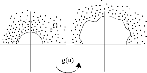
FIG. 2.: The exponentiated domain and its mapping $g(u)$ to the exponentiated physical strip

$g$’s boundary value on $|{\rm Re}u|\geq 1$, Im$u\to 0^{+}$, is real, and just the exponential of pressure along the walls. With no shocks, $p(x,0)$ is continuous. So $g$ takes real rays continuously to real rays. As such it immediately defines its analytic continuation $g(u)\equiv\overline{g(\bar{u})}$ for Im$u<0$, and this reflection symmetric continuation is analytic in the entire $u$-plane for $|u|>1$. With ln and exp both also reflection-symmetric, so too must be $f$:

$$f(\zeta)=\overline{f(\bar{\zeta})}\ ,$$ (27)

as well as $f^{\prime}$ and $f_{t}$. We shall have numerous occasions to utilize this symmetry. Note that the continued $f$ has a domain equivalent to a doubling of the physical problem such that the interface and fluid now enjoy analytically periodic boundary conditions from $-\pi$ to $\pi$. Of course, the physical problem remains in the half strip, but this extra symmetry dictates profound restrictions on $f$’s analyticity structure [14].

D Reflection symmetric equations of motion

Let us now utilize reflection symmetry to transform Eq.(24) into a field equation valid throughout the body of the fluid. Using (27) we can rewrite Eq.(24) in the form

$$2V(t)=f_{t}(\zeta)f^{\prime}(\bar{\zeta})+f_{t}(\bar{\zeta})f^{\prime}(\zeta)\ ,$$ (28)

and noticing that Re$\zeta=0$ implies that $\bar{\zeta}=-\zeta$ we have

$$f_{t}(\zeta)f^{\prime}(-\zeta)+f_{t}(-\zeta)f^{\prime}(\zeta)=2V(t)\ .$$ (29)

It is important to note that this equation holds not just for Re$\zeta=0$, but for all $\zeta$ for which f is analytic. The reason is as follows: solve for $f(\zeta,t)$ from Eq.(24). Compare to the solution of Eq.(29), which we denote temporarily as $\tilde{f}(\zeta,t)$. The two functions $f(\zeta,t)$ and $\tilde{f}(\zeta,t)$ are the same on the boundary Re$\zeta=0$, and since they are analytic they are the same functions. We can thus use (29) instead of (24) for any $\zeta$. Eq.(29) relates $f(\zeta)$ to $f(-\zeta)$ which will prove to be of significant value for the forthcoming analysis. In particular, when $f$ has the elementary analytic behavior $f(\zeta)\sim\zeta$ as Re$\zeta\to\infty$, it follows from (29) that $f$ is analytic as Re$\zeta\to-\infty$. (This is the usual case for the consideration of a sink at $\infty$.)

E A class of solutions

There exist, sprinkled throughout the literature [12, 13, 15], considerations of a class of solutions to (29) with a sink at $\infty$, with moving singularities, most naturally written in $u$-space as

$$g(u)=e^{\beta(t)}u~{}\prod_{k}\left(1-{a_{k}(t)\over u}\right)^{\alpha_{k}}\ .$$ (30)

It is easy to see that for such $g$ the corresponding $f_{t}$ and $f^{\prime}$ simply have poles in $e^{\zeta}$. From the form of (29) we then see that the class of functions $g$ exhausts the solutions of (29) within the class of rational functions of $e^{\zeta}$. We will verify (as has been commented upon in some of the literature [13]) that the equations of motion are satisfied with $\alpha_{k}$ constant in time. Contrary to some of the literature we consider the $\alpha_{k}$ arbitrary complex numbers rather than just real integers [12]. Further, paying attention to the analyticity structure imposed by reflection symmetry, it follows that $\beta(t)$ is real, $|a_{k}(t)|<1$, and for each complex $\{a_{k}(t),\alpha_{k}\}$ pair, there must also be a corresponding pair with both conjugated. Those $g$’s with just one $a$ (which is real and constant in time) comprise the Saffman-Taylor solutions. Numerical explorations in the literature appear to indicate [13] that richer $g$’s replicate a large class of interface motions. (From a numerical point of view a rich enough collection of $a$’s surely serves as a basis.) Some of our comments will follow directly from the equations of motion, whereas others pertain only to arbitrary solutions of the form (30). By the conjugacy (26) we now have for $f$

$$f(\zeta,t)=\beta(t)+\zeta+\sum_{k=1}^{N}\alpha_{k}\ln\left(1-e^{\zeta_{k}(t)-\zeta}\right)\ ,$$ (31)

where $a_{k}(t)\equiv\exp(\zeta_{k}(t))$, Re$\zeta_{k}(t)<0$. We shall suspend until Sect.3 the equations of motion implied by (29) for the parameters of $f$, and further comments on the origin of class (31) in subsection G to follow.

F Elementary flow solutions

Our equations of motion allow for the ready production of a variety of solutions. Consider first the class of solutions with a fixed shape interface uniformly translating in time, so that we can take $V(t)\equiv 1$. The interface is

$$z_{\rm int}(s,t)=f(is,t)=\beta(t)+F(is)\ .$$ (32)

Using (29),

$$f = \beta(t)+F(\zeta);\quad f_{t}=\dot{\beta}(t),\quad f^{\prime}=F^{\prime}(\zeta)$$ (33)

$$\frac{2}{\dot{\beta}} = F^{\prime}(\zeta)+F^{\prime}(-\zeta)\ .$$ (34)

But then, $1/\dot{\beta}\equiv\lambda$, a constant, and $\beta=t/\lambda$. From (34) we deduce

$$F(\zeta)-F(-\zeta)=2\lambda\zeta\ ,$$ (35)

or $f(\zeta,t)-f(-\zeta,t)=2\lambda\zeta$. Setting $\zeta=is$, we find

$$f(is,t)-f(-is,t)=2i\lambda s\ .$$ (36)

By reflection symmetry $f(-is)=\bar{f}(is)$, i.e. Im$f(is,t)=\lambda s$, or

$$y(s,t)=\lambda s\ .$$ (37)

This solution represents an interface that occupies a constant channel fraction, $\lambda$, sensible for $\lambda\in(0,1]$. This also implies that the interface is a graph of $(x(y),y)$, and so conformal for those $\lambda$’s since $|f^{\prime}|>|y^{\prime}|=\lambda$. Writing $F=\lambda\zeta+E(\zeta)$, Eq.(35) is

$$E(-\zeta)=E(\zeta)\ .$$ (38)

The general solution is

$$f=\frac{t}{\lambda}+\lambda\zeta+E(\zeta)\ ,$$ (39)

with $E$ an even function of $\zeta$ compatible with full channel width:

$$\lambda+\frac{1}{\pi i}\left(E(-p+i\pi)-E(-p)\right)=1\ ,$$ (40)

for those curves of constant pressure within the physical fluid ($p<0$) which span the free channel. Since $E$ is even, if $E$ has a singularity at $\zeta_{k}$ with Re$\zeta_{k}<0$, then it must also possess an identical singularity at Re$\zeta_{k}>0$, and so $f$ is no longer analytic in the entire physical fluid, implying the existence of stagnation points or infinite velocities within the fluid itself. Within the class of solutions $g$,

$$f=\frac{t}{\lambda}+\lambda\zeta+\sum\alpha_{k}\ln(1-e^{\zeta_{k}-\zeta})(1-e^{\zeta_{k}+\zeta})$$ (41)

$${\rm Re}\zeta_{k}\geq 0~{}({\rm by~{}definition})\ .$$ (42)

It is expedient, to facilitate the generation of elementary solutions, to consider those solutions which are “periodic” over the physical channel:

$$f(\zeta+i\pi)=f(\zeta)+i\pi\ .$$ (43)

Defining now double-width variables

$$\tilde{\zeta}=2\zeta-i\pi;\quad\tilde{z}=2z-i\pi$$ (44)

so that the physical channel $0\leq$Im$z\leq\pi$ is mapped to $-\pi\leq$Im$\tilde{z}\leq\pi$, we consider

$$\tilde{z} = 2f\left(\frac{\tilde{\zeta}+i\pi}{2}\right)-i\pi\equiv\tilde{f}(\tilde{\zeta})$$ (45)

$$f(\zeta) = \frac{1}{2}\tilde{f}(2\zeta-i\pi)+\frac{i\pi}{2}\ .$$ (46)

$\tilde{f}$ now has $2\pi i$ periodicity, and is again reflection symmetric since $f$ is:

$$\bar{\tilde{f}}(\bar{\tilde{\zeta}})=2\bar{f}\left(\frac{\bar{\tilde{\zeta}}+i\pi}{2}\right)+i\pi=2f\left(\frac{\tilde{\zeta}-i\pi}{2}\right)+i\pi$$ (47)

$$=2f\left(\frac{\tilde{\zeta}+i\pi}{2}-i\pi\right)+i\pi=2f\left(\frac{\tilde{\zeta}+i\pi}{2}\right)-i\pi=\tilde{f}(\tilde{\zeta})\ .$$ (48)

Conversely, any $2\pi i$ periodic reflection symmetric $\tilde{f}$ determines a $\pi i$ periodic reflection-symmetric $f(\zeta)$. (Such an $f$ is too symmetric in that the upper and lower channel walls have perfectly synchronized flows along them, a condition not enforced by the physical data.) The virtue of this device is that an $\tilde{f}$ with just one symmetric pair of singularities produces an $f$ with two symmetric pairs of singularities, and so embraces more complicated flows that does just one symmetric pair.

So far as time-dependence is concerned it is natural to take

$$f(\zeta,t)=\frac{1}{2}\tilde{f}(2\zeta-i\pi,2t)+i\frac{\pi}{2}\quad(\tilde{t}\equiv 2t)\ ,$$ (49)

so that

$$f^{\prime}(\zeta,t)=\tilde{f}^{\prime}(\tilde{\zeta},\tilde{t})\ ,\quad f_{t}(\zeta,t)=\tilde{f}_{\tilde{t}}(\tilde{\zeta},\tilde{t})\ .$$ (50)

Also, by $2\pi i$ periodicity of $\tilde{f}$, $f^{\prime}(-\zeta,t)=\tilde{f}^{\prime}(-\tilde{\zeta},\tilde{t})$ and similarly for $f_{t}$. With $\tilde{V}(\tilde{t})\equiv V(t)$, the equations of motion are covariant. So, all we need do is forget the tildes, solve the simpler problem, and then conjugate it back to the physical space. In the sequel we neglect the last step as an ellipsis the reader readily can fill in. There are reasons to be wary of the extra symmetry in the solutions, and we shall point out this fact when it arises.

The simplest possibility of (42) is one $\zeta_{k}=\pi i$:

$$f = \frac{t}{\lambda}+\lambda\zeta+\alpha\ln(1+e^{-\zeta})(1+e^{\zeta})$$ (51)

$$= \frac{t}{\lambda}+(\lambda+\alpha)\zeta+2\alpha\ln(1+e^{-\zeta})\ .$$ (52)

For full channel width for Re$\zeta>0$, we require $\lambda+\alpha=1$, or

$$f=\frac{t}{\lambda}+\zeta+2(1-\lambda)\ln(1+e^{-\zeta})\quad(f^{\prime}(-\infty)=2\lambda-1)\ .$$ (53)

These are precisely the Saffman-Taylor solutions for a finger of width $\lambda$, and the only such solutions of our class analytic for all Re$\zeta>0$.

The next simplest solution is

$$f = \frac{t}{\lambda}+\zeta+2(1-\lambda)\ln(1+e^{-\zeta})$$ (54)

$$- \alpha\ln(1+e^{-\zeta_{*}-\zeta})(1+e^{-\zeta_{*}+\zeta})\quad(\zeta_{*}>0)\ .$$ (55)

Notice that for $-\zeta_{*}<{\rm Re}\zeta<\zeta_{*}$, the channel is fully occupied with flux, but for Re$\zeta>\zeta_{*}$ the entire asymptotic flux occupies only the fraction $1-\alpha$ of the whole channel. The most interesting such case is $\alpha=1$, when all flux is sunk in the point $f(+\infty)=z_{\rm sink}$:

$$z_{\rm sink}(t)=\frac{t}{\lambda}\ ,\quad f^{\prime}(+\infty)=0\ .$$ (56)

The constant pressure contours for $0>p>-\zeta_{*}$ span the channel, but those for $p<-\zeta_{*}$ are closed curves surrounding the sink at $z_{\rm sink}$. The separatrix between them at $\zeta=\zeta_{*}+is$ has the form

$$z_{*} = \frac{t}{\lambda}+\zeta_{*}+is+2(1-\lambda)\ln(1+e^{-\zeta_{*}-is})$$ (57)

$$- \ln(1+e^{-2\zeta_{*}-is})-\ln(1+e^{is})\ .$$ (58)

For $\zeta_{*}\gg 1$

$$z_{*}\approx\frac{t}{\lambda}+\zeta_{*}+is-\ln(1+e^{is})\ ,$$ (59)

and is an upstream-pointing Saffman-Taylor finger of width $2(1-\lambda)=1$, or $\lambda=1/2$, by comparison to (53), see Fig.3.

FIG. 3.: Schematic stream and pressures lines in a channel with an advancing finger (shaded region) and a sink (denoted by $\times$). The stream and pressure lines are indicated by dashed and continuous curves respectively. The pressure line with $p=p^{*}$ separates pressure lines that connect the walls (like $p_{a}$) and those which form closed curves around the sink (like $p_{b}$). The stream lines $s=\pi,\bar{s}=-\pi$ graze the walls $y=\pm\pi$ respectively from $x=-\infty$ to $x=\infty$ where they curve around and return along $y=0^{+}$ and $y=0^{-}$ respectively from $x=\infty$ to the sink, forming a branch cut.

This is amusing, and suggests that with an enforced symmetry between $\zeta$ and $-\zeta$, then (56) would be $f^{\prime}(-\infty)=0$, so that if (53) were asymptotically valid, then a $1/2$ width finger for the interface itself could be implied. We will return to these matters later.

Let us now consider some elementary solutions with variable flux $V(t)$. The simplest solution arises when the pressure profiles are a function of $x$ but not of $y$, $p=p(x,t)$. This implies, by analyticity, that

$$f=\beta(t)+\zeta\ ,$$ (60)

where the coefficient 1 of $\zeta$ specifies a channel fully occupied with flux. We now pose finite boundary conditions, namely that $p=p_{a}$ (atmospheric pressure) on $x=L$. We denote $p_{g}=|p_{a}|$, and write $2L=f(\zeta)+f(\bar{\zeta})$, on $2p_{g}/V=\zeta+\bar{\zeta}$. Accordingly

$$2L=f(\zeta)+f(\frac{2p_{g}}{V}-\zeta)=2\beta+\frac{2p_{g}}{V}\ ,$$ (61)

or $L=\beta+p_{g}/V$. Using the fact that in this case $\dot{\beta}=V$, we need to solve the differential equation

$$\beta\dot{\beta}-L\dot{\beta}+p_{g}\ .$$ (62)

The solution is $\beta^{2}-2L\beta+2p_{g}t=const$. Choosing initial conditions such that the interface is at zero when $t=0$ determines $x_{\rm int}=\beta=L-\sqrt{L^{2}-2p_{g}t}$. For the velocity we find

$$V=\dot{\beta}={p_{g}\over\sqrt{L^{2}-2p_{g}t}}\ .$$ (63)

This makes it clear that any genuine physical determination of the flow (including the flux) requires boundary conditions at finite pressures, rather than at $p\to-\infty$.

G The class of solutions (27) as a resummation

Before turning to the discussion of analyticity and conformality of the solutions, it is important to reflect on the meaning of these solutions. It is straightforward to verify that if we start with a Saffman-Taylor solution with width 1/2, that is,

$$f_{0}=2t+\ln(e^{\zeta-\hat{\zeta}}+1)\ ,\quad e^{-2\hat{\zeta}}=1+e^{-2t}$$ (64)

and perturb it to say $f_{0}+\epsilon f$, then the equations of motion are satisfied with errors $O(\epsilon^{2})$, for each

$$f_{n}=e^{2nt}(1+e^{-\hat{\zeta}-\zeta})^{n}\ ,\quad n=1,2,\dots\ ,$$ (65)

all analytic as Re$\zeta\to\infty$. That is, the basis for perturbations to $f_{0}$ grow exponentially in time. We can construct from these, “center manifold” perturbations that grow slower than exponential in time, by forming the infinite sum

$$f_{a} = -\sum_{1}^{\infty}(-a)^{n}f_{n}=\ln(1+ae^{2t}(1+e^{-\hat{\zeta}-\zeta}))$$ (66)

$$= \ln(1+ae^{2t})+\ln(1+e^{\zeta_{s}(t)-\hat{\zeta}})$$ (67)

$$\zeta_{s} = -\hat{\zeta}-\ln(1+e^{-2t}/a)\ .$$ (68)

(For $a=1$, $\zeta_{s}=\hat{\zeta}$). Thus, class (31) viewed as $f_{0}$ plus fluctuations, is simply an infinite resummation of the unstable manifold spanned by (65). But this makes it clear that generic functions are to obtained, reciprocally, by infinite summations over class (31), they behaving very differently from a finite sum. This leaves as open the issue if conclusions based on class (31) have any unrestricted applicability. This question is beyond the scope of this paper, and will be addressed in a future paper.

3 Analyticity and conformality as a function of time

A Solutions of the equations of motion for the class $g$ and asymptotic stagnation points

Considering the solution (31) we compute

$$f_{t} = \dot{\beta}-\sum_{k=1}^{N}{\alpha_{k}\dot{\zeta}_{k}\over e^{\zeta-\zeta_{k}}-1}$$ (69)

$$f^{\prime} = 1+\sum_{k=1}^{N}{\alpha_{k}\over e^{\zeta-\zeta_{k}}-1}$$ (70)

It is useful to consider these equations in various limits. Consider first $\zeta\to\pm\infty$ on the real axis:

$$\zeta\to\infty:\quad f_{t} = \dot{\beta}\quad f^{\prime}=1\ ,$$ (71)

$$\zeta\to-\infty:\quad f_{t} = \dot{\beta}+\sum_{k}\alpha_{k}\dot{\zeta}_{k}$$ (72)

$$f^{\prime} = 1-\sum_{k}\alpha_{k}\ .$$ (73)

Substituting in the equation of motion (29) we find

$$(2-\sum_{k}\alpha_{k})\beta+\sum_{k}\alpha_{k}\zeta_{k}=2(t-t_{0})\ ,$$ (74)

with $t_{0}$ a constant of integration. Next consider the asymptotic behavior $\zeta\sim\zeta_{k}$:

$$\zeta\sim\zeta_{k}:\quad f_{t}\sim-{\alpha_{k}\dot{\zeta}_{k}\over e^{\zeta-\zeta_{k}}-1}\ ,\quad f^{\prime}\sim{\alpha_{k}\over e^{\zeta-\zeta_{k}}-1}$$ (75)

Substituting in the equation of motion (29), after dividing by $f^{\prime}(\zeta)f^{\prime}(-\zeta)$, we find

$$-\dot{\zeta}_{k}f^{\prime}(-\zeta_{k},t)+f_{t}(-\zeta_{k},t)=0\ .$$ (76)

(Had we taken the $\alpha_{k}$ time dependent the first sub-dominant asymptotic term would have revealed that indeed the $\alpha_{k}$ are constant.) Recognizing that this equation reads $df(-\zeta_{k},t)/dt=0$, we introduce the points $z_{k}$ in physical space,

$$\bar{z}_{k}\equiv f(-\zeta_{k},t)\ ,\quad\dot{z}_{k}=0\ .$$ (77)

(Notice that by reflection symmetry $z_{k}$, as the $\zeta_{k}$, come in complex conjugate pairs.) With Re$\zeta_{k}<0$ we see that $-\zeta_{k}$ is in the interior of $\Omega$, and therefore $z_{k}$ is within the moving fluid. Thus $z_{k}$ are asymptotic stagnation points of the flow as the singularities approach the interface. This result was observed for the first time in [13]. More correctly, the fluid stagnates $\alpha_{k}\ln 2$ upstream from $z_{k}$ as Re$\zeta_{k}\to 0$, at $\zeta=i$Im$\bar{\zeta}_{k}$. Finally we rewrite Eq.(77) in the form

$$\bar{z}_{k}=\beta(t)-\zeta_{k}+\sum_{l}\alpha_{l}\ln(1-e^{\zeta_{l}+\zeta_{k}})\ .$$ (78)

B Necessary Conditions for Asymptotic Analyticity

The discussion of analyticity is largely independent of the explicit form of solutions (31). Infinite channel asymptotics implies that

$$f=\beta+\zeta+F(\zeta,t)\ ,$$ (79)

with the first two terms describing a uniformly translating fluid, and the last term its decoration, (exponentially) vanishing at $+\infty$, so that

$$F,~{}F^{\prime},~{}F_{t}\to 0~{}{\rm as~{}Re}\zeta\to+\infty\ .$$ (80)

Much of the discussion relies just on this. Moreover, to exhibit the moving singularities, we write

$$F(\zeta,t)=\sum F_{k}(\zeta-\zeta_{k}(t))\ ,~{}~{}F_{t}=-\sum\dot{\zeta}_{k}F^{\prime}_{k}(\zeta-\zeta_{k}(t))\ ,$$ (81)

with each $F_{k}$ obeying (80), and by the analyticity of $f^{\prime}$ at$-\infty$,

$$F^{\prime}_{k}(-\infty)\equiv-\alpha_{k}\ .$$ (82)

Granted this level of detail of $f$’s form, we have by the equations of motion(29), with $f\sim\beta+\zeta$ as Re$\zeta\to+\infty$,

$$f_{t}(-\infty)+\dot{\beta}f^{\prime}(-\infty)=2\ ,$$ (83)

or

$$(1+f^{\prime}(-\infty))\dot{\beta}+F_{t}(-\infty)=2\ ,$$ (84)

or

$$(1+f^{\prime}(-\infty))\dot{\beta}+\sum\alpha_{k}\dot{\zeta}_{k}=2\ ,$$ (85)

or

$$(1+f^{\prime}(-\infty))\beta+\sum\alpha_{k}\zeta_{k}=2(t-t_{0})\ .$$ (86)

Let us write

$$1+f^{\prime}(-\infty)=2-\sum\alpha_{k}\equiv 2\lambda\ .$$ (87)

Should all work well, with no impediment against all the $\zeta_{k}$ approaching the interface Re$\zeta=0$ as $t\to\infty$, then (86) implies

$$\beta\sim{t\over\lambda}\ .$$ (88)

It is now straightforward to show that the physical case requires

$$0<\lambda<1\ ,$$ (89)

and hence by (87)

$$|f^{\prime}(-\infty)|<1\ .$$ (90)

To see this, let us determine $\zeta(\zeta_{0},t)$ for Re$\zeta\to+\infty$. The differential equation for $\zeta$, Eq.(23) reads here

$$1\sim\zeta_{t}+\dot{\beta}\ .$$ (91)

Integrating

$$\zeta\sim t-\beta+\zeta_{0}\sim(1-{1\over\lambda})t+\zeta_{0}\ .$$ (92)

A given, far downstream, $\zeta_{0}$ lies on a line of constant pressure, imaged by $f$ at $t=0$ into a curve in $z$-space of constant pressure. Should $\zeta(\zeta_{0},t)$ at later times be further downstream, then by (79) and (80) this same fluid particle lies on successively flatter pressure curves, so that a flattening profile propagates upstream towards the interface. Of course, precisely the opposite must occur, and so by (92)

$$1-{1\over\lambda}<0\ ,\quad{\rm or}~{}0<\lambda<1\ .$$ (93)

With $\zeta$ of (92), we now know the trajectories of far downstream particles:

$$f(\zeta,t)\sim\beta+\zeta\sim t+\zeta_{0}\ ,$$ (94)

just reflecting uniform unit flux of the fluid. On the other hand, with the interface at Re$\zeta=0$ and Re$\zeta_{k}\to 0^{-}$, $F$ is bounded outside sufficiently small disks about the $\zeta_{k}$’s, and so $F(is,t)$ is bounded outside sufficiently small intervals of $s$. Observing Eq.(69) and realizing that for long times $\dot{\zeta}_{k}\to 0$, (and see a formal proof in the next section), we reach the conclusion that

$$f(is)\sim\beta\sim{t\over\lambda}$$ (95)

and so the interface is moving at velocity $1/\lambda>1$. Conservation of flux then imposes that the net width of the moving interface is just $\lambda$ times the full channel width, which to be physical (not to fail $h$’s conformality) must lie between 0 and 1. It is thus clear that of all possible $f$’s, only those obeying (90) meet physical boundary conditions. We next show that for just these $f$’s analyticity is never lost in finite time.

C Absence of Violations of Analyticity

We prove now that the solutions do not lose analyticity so long as (90) is obeyed. $f$ can fail to be analytic in the physical region in two possible ways: either $|\beta|$ diverges, leaving $f$ defined nowhere, or the moving singularities cross Re$\zeta=0$ into the physical regime. By presumption, $\beta$ is finite and Re$\zeta_{k}<0$ at $t=0$, so that until such a disease occurs, Re$\zeta_{k}$ are bounded from above. We shall now demonstrate $f$’s analyticity for all future times by exhausting the possibilities. First, consider that some of the $\zeta_{k}$’s tend to $-\infty$ at some finite or infinite time. Call the set of all such indices $k$ $\tilde{S}$, and its complement, $S$, then the set of singularities remaining bounded. We show $\tilde{S}$ is empty without proviso. According to the equations of motion for the singularities, for $\zeta_{k}\to-\infty$, by (79) and (80)

$$\bar{z}_{k}=f(-\zeta_{k})\sim\beta-\zeta_{k}\ ,\Rightarrow~{}\beta\to-\infty$$ (96)

and produces a disease. But then

$$\sum_{\tilde{S}}\alpha_{k}\zeta_{k}\sim\beta\sum_{\tilde{S}}\alpha_{k}+bdd$$ (97)

and by (86) and (87)

$$2t\sim\beta(2-\sum_{k}\alpha_{k})+\beta\sum_{\tilde{S}}\alpha_{k}+bdd=\beta(2-\sum_{S}\alpha_{k})+bdd\ .$$ (98)

Should $2-\sum_{S}\alpha=0$ this can (potentially) occur at finite time, else as $t\to\infty$, $2-\sum_{S}\alpha<0$ ($\beta\to-\infty$). That is, we require

$$\sum_{S}\alpha\geq 2\ .$$ (99)

Now, consider $\zeta_{k}$ with any $k\in S$. From (77) and (79)

$$\bar{z}_{k}=\beta-\zeta_{k}+\sum_{\ell}F_{\ell}(-\zeta_{k}-\zeta_{\ell})\sim\beta+\sum_{\ell\in S}F_{\ell}(-\zeta_{k}-\zeta_{\ell})\ ,$$ (100)

or, with $\beta\to-\infty$

$$\sum_{\ell\in S}F_{\ell}(-\zeta_{k}-\zeta_{\ell})\to+\infty,~{}{\rm for~{}each}~{}k\in S\ .$$ (101)

Eq.(101) can be satisfied only if $\zeta_{k}+\zeta_{\ell}\to 0,\pm 2\pi i$ so that $F_{\ell}$ becomes singular, i.e. when all the Re$\zeta_{k}\to 0^{-}$, $k\in S$. Define

$$S_{k}\equiv\{\ell|\bar{\zeta}_{k}+\zeta_{\ell}\to 0,\pm 2\pi i\}\ .$$ (102)

Clearly, $k\in S_{k}$, so that no $S_{k}$ is empty, and the $S_{k}$’s are a partition of $S$. Then, (101) is

$$\sum_{\ell\in S_{\bar{k}}}F_{\ell}(-\zeta_{k}-\zeta_{\ell})\to+\infty\ .$$ (103)

Here we use a detail of $F_{\ell}$ of (31): the logarithm tends to $-\infty$, and so (103) requires

$${\rm Re}\sum_{\ell\in S_{\bar{k}}}\alpha_{\ell}<0\ ,$$ (104)

where $\zeta_{\bar{k}}\equiv\bar{\zeta}_{k}$. Summing (104) over distinct $S_{\bar{k}}$, we then have

$$\sum_{S}\alpha={\rm Re}\sum_{S}\alpha<0\ ,$$ (105)

but this contradicts (99). Finally should $S$ be empty, (all $\zeta_{k}\to-\infty$), (98) is $t\sim\beta$, impossible since $t>0$. We thus conclude that no $\zeta_{k}$ can go to $-\infty$ for any $t>0$. We are now left with the circumstance that all $\zeta_{k}$ are bounded. Should $\beta$ be finite, then it is impossible for any $\zeta_{k}$ to cross Re$\zeta=0$. This is contingent upon $F_{k}$ imaging an arbitrarily small disc about $\zeta_{k}$ with arbitrarily large modulus, such as is the case for $F_{k}$ of (31) with Re$\alpha_{k}\neq 0$. In this circumstance, and with $\beta$ finite, $|f(\zeta_{k})|\to\infty$, $|f(-\bar{\zeta}_{k})|=|z_{k}|=$finite, and so $\zeta_{k}$ cannot approach $-\bar{\zeta}_{k}$, i.e. Re$\zeta_{k}$ cannot approach 0. Accordingly the discussion has contracted to Re$\zeta_{k}\to 0$, $|\beta|\to\infty$, for which (98) reads

$$2t\sim\beta(2-\sum\alpha_{k})=\beta(1+f^{\prime}(-\infty))\ .$$ (106)

Should $f^{\prime}(-\infty)=-1$, then $\beta$ can diverge at finite $t$, and generally a finite-time loss of analyticity can occur. Otherwise we have just $t\to+\infty$ , and so,

$$f^{\prime}(-\infty)<-1\ ,\quad\beta\to-\infty\ ,$$ (107)

or

$$f^{\prime}(-\infty)>-1\ ,\quad\beta\to+\infty\ .$$ (108)

(Since $|\beta|\to\infty$, every $\zeta_{k}$ crosses Re$\zeta=0$ “simultaneously” at $t=+\infty$.) Should case (107) hold the argument leading to (105) is appropriate, save that $S$ includes all the $\zeta_{k}$’s, and so $\sum\alpha_{k}<0$, i.e., $f^{\prime}(-\infty)>1$, a contradiction to (107). Thus, only case (108) remains, in which case, the same argument leading to (105) is now $\sum\alpha_{k}>0$, i.e. $f^{\prime}(-\infty)<1$, which with (108) is $|f^{\prime}(-\infty)|<1$. To summarize what we have now demonstrated,

Observation 1: Unless $f^{\prime}(-\infty)=-1$, then $f$ remains analytic throughout the physical region for all positive time. $t$ can only continue to $+\infty$ if $|f^{\prime}(-\infty)|<1$.

The curious part of this result is that if $|f^{\prime}(-\infty)|>1$, then $f$ remains analytic, but the $\zeta_{k}$ never get to cross Re$\zeta$=0. This happens because then $f$ must lose conformality because $f_{t}$ has diverged (i.e. $\dot{\beta}$ and $\dot{\zeta}_{k}$’s become infinite) although $f$ is finite and analytic at such an instant. Should $f_{t}$ diverge, then the equations of motion imply that $f^{\prime}=0$ at some point on the interface, i.e. that $v\to\infty$ at some point of the physical fluid. What our observation says is there must surely be finite-time singularities should $|f^{\prime}(-\infty)|>1$. These singularities represent precisely an impending violation of boundary conditions. To see this, recall that our wall boundary conditions are $x_{s}(p,s)=0$ on $s=0,\pi$. By reflection symmetry, $f$ has been analytically continued to $-\pi<s<\pi$, rather than just the physical $0<s<\pi$. However such an $f$ does not necessarily map $s>0$ to just $y>0$. It will do so provided that $f$ is conformal. Should $f$ not be a contraction at $-\infty$, it is inevitable that, as the singularities approach the interface, $f$ will begin to map across half channels, and so, such an $f$ fails physical boundary conditions, and so is not an admissible solution. (To see this, by Eq.(26), $g^{\prime}/g=f^{\prime}/u$, or $g\sim u^{f^{\prime}(-\infty)}$ as $u\to 0$- i.e. everywhere within the radius of that $a_{k}(t)$ with smallest modulus. That is,with arg$u=\phi$, arg$w\sim f^{\prime}(-\infty)\phi$, and exceeds half channel width unless $|f^{\prime}(-\infty)|<1$.) Consequently our observation reads that all admissible solutions under physical channel boundary conditions are free from finite time failures of analyticity, so that the conformal machinery we are employing is perfectly applicable. The difficulty is, while $|f^{\prime}(-\infty)|>1$ always leads to finite time failures in $f$’s conformality, the same disease can arise for admissible solutions as well. This difficulty is profound, and we will expand upon it in the next section.

4 The asymptotics and the emergence of One Finger

We are ready now to establish a significant result: For $t\to\infty$ the physical channel supports one finger. In the doubled channel, that is considered in all the literature, this of course means two fingers with a stagnation point on the symmetry line. In particular, one finger in this geometry is a physically incorrect result. Mathematically this is equivalent to the following

Observation 2: For solutions that do not lose conformality for $t\to\infty$, and for which all $\alpha_{k}$ are generic with Im$\alpha_{k}\neq 0$, all $\zeta_{k}\to 0,\pm i\pi$.

Demonstration: Consider one of the terms in the sum (31), say $\alpha_{k}\ln\left(1-e^{\zeta_{k}-\zeta}\right)$. Consider a circle of radius $|\epsilon|$ around the singularity, $\zeta=\zeta_{k}+\epsilon$, where $\epsilon\equiv|\epsilon|e^{i\phi}$, $|\epsilon|$ is small, and $-\pi<\phi<\pi$. We investigate the image of this small circle under $f$. For small $|\epsilon|$

$$f\sim\beta(t)+\alpha_{k}(\ln|\epsilon|+i\phi)~{}{\rm mod}\pm i\pi\ .$$ (109)

For a given $|\epsilon|$ this image is a line of length $2\pi|\alpha_{k}|$ perpendicular to the direction of $\alpha_{k}$ (see Fig. 3). Consider next the punctured disk around the singularity with radius $|\epsilon|$. This disk is imaged onto a series of slanted strips ordered along the direction of $\alpha_{k}$ with the above width as shown in Fig.4.

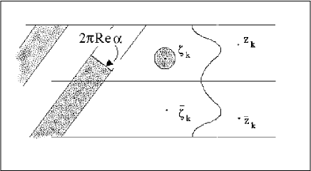
FIG. 4.: The mapping of a neighborhood of one of the singularities

As time progresses and $\beta$ increases, this series moves to the right, entering the physical domain. (Remember, this is a neighborhood of a singularity, not a singularity!). Eventually, when $|$2Re$\zeta_{k}|<|\epsilon|$ the image of a very small $|\epsilon|$-neighborhood of $\zeta_{k}$ must include the stagnation point $z_{k}$, the fixed image of $-\bar{\zeta}_{k}$, and must for all future time always include it. But as $t$ increases, the fixed width strip containing $z_{k}$ is moving arbitrarily far to the right. This would seem impossible. The only way to resolve this conundrum is that

$$\zeta_{k}(t)\to 0~{}{\rm or}~{}\pm i\pi\quad{\rm as}~{}t\to\infty\ .$$ (110)

When this happens $e^{\zeta_{k}}\to e^{\bar{\zeta}_{k}}$ and $\bar{\zeta}_{k}$ (mod $2\pi i$ if necessary) is also in the $|\epsilon|$-neighborhood, and its term in (31) must be also included in (109). But

$$\alpha\ln(1-e^{\zeta_{k}-\zeta})+\bar{\alpha}\ln(1-e^{\bar{\zeta}_{k}-\zeta})\to 2{\rm Re}\alpha\ln(1-e^{\zeta_{k}-\zeta})\ .$$ (111)

and so the strips begin to rotate to the horizontal, and sufficiently so that $z_{k}$ always remains within its strip. (110) is the only way to have Re$\zeta_{k}\to 0$.

It should be stressed that even though an asymptotic finger solution is emerging, its width is in no way selected. Moreover, over the duration of an actual experiment, not all the singularities need be yet in asymptotic proximity to Re$\zeta=0$. That is, a subset of $\zeta_{k}$’s of the same order of magnitude will carry out migration toward 0 or $i\pi$, while other sets with extremely large -Re$\zeta_{k}^{\prime}$ are still very far from asymptotic behavior.

To see this, consider as usual $f$ of (27) built from those $\zeta_{k}$ that are sufficiently close to one another, and consider an exponentially small perturbation, built from $\zeta_{k}^{\prime}$ with Re$\zeta_{k}^{\prime}\leq-x\ll$ Re$\zeta_{k}$, $x\gg 1$:

$$f=\beta+\zeta+\sum\alpha_{k}\ln(1-e^{\zeta_{k}-\zeta})+\sum\alpha_{k}^{\prime}\ln(1-e^{\zeta_{k}^{\prime}-\zeta})\ .$$ (112)

Clearly, near the interface the last term is $O(e^{-x})$. Writing the equations for $\zeta_{k}^{\prime}$,

$$\bar{z}_{k}^{\prime}=\beta-\zeta_{k}^{\prime}+O(e^{-x})\ ,\quad\rightarrow{\rm Re}\bar{z}_{k}^{\prime}\geq\beta+x\ .$$ (113)

Writing the $\beta$ equation

$$(1-\sum\alpha_{k})\beta + \beta+\sum\alpha_{k}\zeta_{k}$$ (114)

$$+ (\sum\alpha_{k}^{\prime}\zeta_{k}^{\prime}-\beta\sum\alpha_{k}^{\prime})=2t-k\ .$$ (115)

Multiplying each equation of (113) by the $\alpha_{k}^{\prime}$ and summing, we see, with $k=\sum\alpha_{k}^{\prime}\bar{z}_{k}^{\prime}$,

$$(1-\sum\alpha_{k})\beta+\beta+\sum\alpha_{k}\zeta_{k}=2t+O(e^{-x})\ ,$$ (116)

while the equations for each $\zeta_{k}$ are

$$\bar{z}_{k}=\beta-\zeta_{k}+\sum\alpha_{\ell}\ln(1-e^{\zeta_{k}+\zeta_{\ell}})+O(e^{-x})\ .$$ (117)

We see then, by (116) and (117) that the near set of $\zeta_{k}$’s, for $x$ large enough, behaves exactly as a full system, and forms a finger of width $\lambda=1-\sum\alpha_{k}/2$, and $\beta=t/\lambda$. But then, by (113), for $t\leq\lambda x/2$, Re$\zeta_{k}^{\prime}<-x/2$, and the $\zeta_{k}^{\prime}$ still play an exponentially small role up to very long times during which a $\lambda$-finger is propagating. Ultimately for $t\sim\lambda x$, the $\zeta_{k}^{\prime}$ become asymptotic, and the finger metamorphoses into a $\lambda^{\prime}=1-(\sum\alpha_{k}+\sum\alpha_{k}^{\prime})/2$. So, from a physical viewpoint, with $\sum\alpha_{k}+\sum\alpha_{k}^{\prime}=1$, the finger will become $\lambda=1/2$ long after the experiment is over. But $f^{\prime}(-\infty)=1-\sum\alpha-\sum\alpha^{\prime}=0$ no matter how large $x$ may be. We see from this that $f^{\prime}(-\infty)=0$ is insufficient to determine $\lambda=1/2$. The width is determined just by the $\zeta_{k}^{\prime}$s near enough to Re$\zeta=0$. Indeed, in (112) the $\sum\alpha_{k}^{\prime}$ can be chosen arbitrarily with no consequence during the experiment. Note that (112) is the transparent implementation of the manipulations of [7]. It is clear that [7] then has no significance for selection of a 1/2 finger. (By choosing the $\sum\alpha^{\prime}$ arbirtrarily, the argument of [7] would then show the “selection” of any $\lambda$ whatever.) These comments pose a limitation on Observation 2 as well: The larger the number of $\zeta_{k}$’s we choose, the more semi-asymptotic regimes the initial conditions can be chosen to determine, so that in the limit as this number diverges, no final asymptotics need exist.

5 Violations of conformality: finite time singularities

The discussion that follows critically assumes that $f$ is in the manifold (31). Should the velocity of a fluid point diverge, $h^{\prime}\to\infty$ and correspondingly $f^{\prime}\to 0$, and so the map $f$, while remaining analytic, has locally lost conformality. As we observed at the end of Sect. 3.c, should $|f^{\prime}(-\infty)|>1$, for infinite channel flow, then there must occur a violation of conformality. However, this circumstance is trivial, in that we realized the failure occurred on the walls of the channel, and hence is not a solution under our boundary conditions. Regrettably, this is far from the only way in which such violations occur. However, it is not too hard to determine when $f^{\prime}(\zeta)=0$ for some $\zeta$ within the physical fluid. Since for infinite channel flow $f^{\prime}(\infty)=1$, and so long as $f^{\prime}(\zeta)\neq 0$ for Re$\zeta\geq 0$, then $|f^{\prime}(\zeta)|>0$ throughout the physical region. But then $|f^{\prime}|$, since $f^{\prime}$ is analytic, has its minimum value over a region on the boundary of that region, which now evidently means the interface at Re$\zeta$=0. It now follows that if a failure of conformality occurs, it must first appear on the interface, and so the condition for a finite-time singularity is

$$f^{\prime}(is)=0$$ (118)

for some $0<s<\pi$ (but not a boundary violation at 0 or $\pi$).

To understand what happens, consider the behavior of the Saffman- Taylor solutions, that is $N=1$ in (31). By (74)

$$\beta={2t\over 2-\alpha}-{\alpha\rho_{0}\over 2-\alpha}\ ,$$ (119)

where the one singularity, $\rho_{0}$, is real as is its corresponding $\alpha$. Then, by (78), with $z_{0}=0$,

$$0={2(t-\rho_{0})\over 2-\alpha}+\alpha\ln(1-e^{2\rho_{0}})$$ (120)

or

$$t=\rho_{0}-{1\over 2}\alpha(2-\alpha)\ln(1-e^{2\rho_{0}})\ .$$ (121)

(121) is soluble for $\rho_{0}$ as long as $t^{\prime}(\rho_{0})\equiv dt/d\rho_{0}\neq 0$. For $\rho_{0}\to-\infty$, evidently $t\sim\rho_{0}$ and $t$ can increase from the far past. For $t^{\prime}=0$, generally, $t$ will have then a maximum, and so $\dot{\rho}_{0}\to\infty$, inducing a finite time singularity. But

$$t^{\prime}=0=1+{\alpha(2-\alpha)\over e^{-2\rho_{0}}-1}\ ,$$ (122)

or

$$e^{-2\rho_{0}}=(1-\alpha)^{2}=[f^{\prime}(-\infty)]^{2}\ ,\quad e^{-\rho_{0}}=|f^{\prime}(-\infty)|\ .$$ (123)

We now see that with $\rho_{0}<0$, $t^{\prime}=0$ is impossible for $|f^{\prime}(-\infty)|<1$, but certain otherwise. That is, time “locks” for the inadmissible cases, and only these cases. With $\dot{\rho}\to\infty$ (but f finite and analytic), $f_{t}\to\infty$, and we seek a $\zeta$ on the interface where $f^{\prime}(\zeta)=0$. But

$$f^{\prime}=0=1+{\alpha\over e^{\zeta-\rho_{0}}-1}\ ,$$ (124)

or

$$e^{\zeta}=(1-\alpha)e^{\rho_{0}}={f^{\prime}(-\infty)\over|f^{\prime}(-\infty)|}=\pm 1\ .$$ (125)

This is the general nature of the failure of conformality. At some time, $t_{0}$, time locks and various of $\dot{\beta}$ and $\dot{\zeta}_{k}$ diverge, and hence $f_{t}$ diverges, although $f$ can be perfectly finite. Simply, the system (74),(78) becomes locally non-invertible for the $\zeta_{k}$’s.

We noticed in Sect.2.F that Re$f^{\prime}(\zeta)=\lambda$ for our translating solutions so that $|f^{\prime}(\zeta)|=\lambda>0$, and the interface is conformal, and any violation of conformality is the interior representation of sinks or sources. But Re$f^{\prime}(is)=y^{\prime}(s)$, or $y=\lambda s$, and so $x(s)=X(y)$, and the interface is a graph of $x$ on $y$. Generally, a graph with finite $X^{\prime}(y)$ (i.e. a differentiable graph) won’t fail conformality.

For the class of solutions in Sect 2.E with all $\alpha_{k}>0$, it is easy to see that $y^{\prime}(s)>\lambda$, and so $y$ is monotone in $s$, and hence the solution is a graph with $|f^{\prime}(\zeta)|>\lambda$ and so always conformal for $0<\lambda<1$. The only possibility for a failure of conformality is with complex $\alpha$’s and the interface, a graph in the far past, about to become not a graph. (Indeed, the generic rotation mechanism for the emergence of one asymptotic finger is Im$\alpha_{k}\neq 0$ for all $k$.) Real time singularities thus can arise when a “balloon” (not a graph) is about to form.

With $\alpha_{k}=a_{k}+ib_{k}$, Re$f^{\prime}(is)$ is modified with $b_{k}\neq 0$ by terms exponentially small when the singularities are far from Re$\zeta$=0, that is $\sim e^{{\rm Re}\zeta_{k}}$. Thus conformality can fail only when singularities enter the rotation mechanism of Sect.4, which turns fingers into balloons. In particular, this is definitely beyond the perturbative regime, and when the nonlinearities have become very strong. The usual linear stability analysis, with temporal exponents proportional to wavelength, simply means that fluctuations very rapidly bring the solution into the strongly nonlinear regime. Indeed, rather than infinitely wrinkled, distorted interfaces, if the rotation mechanism can work, a smooth single balloon is the consequence of the nonlinearities, provided class (31) obtains. We will have more to say about this in [8], as it transpires that the unstable bhavior of the infinite channel is physically significantly wrong. Any inspection of early interface structure - say in Saffman-Taylor’s original paper - reveals that it is balloons that are pervasive, and not graphs or fingers. Let us consider the simplest balloon.

With the channel-doubling conjugacy of Sect. 2.F implicit, consider the solutions with one $\zeta_{k}$:

$$f = \beta+\zeta+\alpha\ln(1-e^{\zeta_{0}-\zeta})+\bar{\alpha}\ln(1-e^{\bar{\zeta}_{0}-\zeta})$$ (126)

$$\alpha = a+ib;~{}~{}a,b>0;~{}~{}\zeta_{0}\equiv-\xi+i\eta,\xi>0\ .$$ (127)

The equation of motion $z_{0}=f(-\bar{\zeta}_{0})$ is

$$z_{0} = \beta-\bar{\zeta}_{0}+\alpha\ln(1-e^{2{\rm Re}\zeta_{0}})+\bar{\alpha}\ln(1-e^{2\bar{\zeta}_{0}})$$ (128)

$$z_{0} = \beta+\xi+i\eta+\alpha\ln(1-e^{-2\xi})+\bar{\alpha}\ln(1-e^{-2\xi-2i\eta})\ .$$ (129)

Its imaginary part is

$$y_{0}=\eta+a{\rm Arg}(e^{2\xi}-e^{-2i\eta})-\frac{b}{2}\ln{|e^{2\xi}-e^{-2i\eta}|^{2}\over(e^{2\xi}-1)^{2}}\ ,$$ (130)

or

$$y_{0}=\eta+a\tan^{-1}{\sin 2\eta\over e^{2\xi}-\cos 2\eta}-\frac{b}{2}\ln(1+{\sin^{2}\eta\over\sinh^{2}\xi})\ .$$ (131)

with the usual principal value of $\tan^{-1}$ correct. $y_{0}$ is here half the distance between the two “stagnation” points $z_{0}$ and $\bar{z}_{0}$. The level curves of the RHS of (131) with $0\leq y_{0}\leq\pi$ are precisely, for each $y_{0}$, the trajectory curve of a $\zeta_{0}$, however it be parametrized by $t$. There are three types of trajectories that connect to $\xi\to\infty$ (with $y\to y_{0}$ as $\xi\to\infty$):
(i) $\tan^{-1}\frac{a}{b}<y_{0}\leq\pi$: the trajectory monotonically (in -$\xi$) increases from $y_{0}$ to $\pi$ as $\xi\to 0$.
(ii) $a\tan^{-1}\frac{a}{b}-\frac{b}{2}\ln(1+\frac{a^{2}}{b^{2}})<y_{0}<\tan^{-1}\frac{a}{b}$: the trajectory moves from $y_{0}$ to $\pi$ as $\xi\to 0$, initially to lower $\eta$ values, and with a unique minimum.
(iii) $0\leq y_{0}<a\tan^{-1}\frac{a}{b}-b\ln(1+\frac{a^{2}}{b^{2}})$: the trajectory monotonically flows from $y_{0}$ to $0$ as $\xi\to\infty$.

Trajectories of types (i) and (ii) rotate to $\pi$, and the “walls” at $\pm\pi$ are closed to flow, with a balloon symmetric about $y=0$ moving down the channel. Type (iii) has $\zeta_{0}$ and $\bar{\zeta}_{0}$ both rotate to $\eta=0$, blocking flow along $y=0$, with fluid advancing along the $\pm\pi$ walls. By Sect.2.F, (i) and (ii) have blocked flow at $y=0,\pi$ with the balloon symmetric about $y=\pi/2$, while (iii) has flow blocked along $\pi/2$, since the upper half poles are both rotating together to $\pi/2$. This is unphysical and non-generic: the rotation mechanism of Sect.4 can only lead to this under extra, nonphysical, symmetry, which of course is exactly what the method of Sect.2F creates. With two generic poles, case (iii) would not have occurred. Regrettably, this generic version is not analytically tractable.

However, while it turns out that type (iii) never encounters finite time singularities, not all the “good” types, (i) and (ii) trajectories are free of disease. That is, there is, for each $a$ and $b$, a minimum gap, $2y_{0}^{\rm min}$ between the stagnation points that allows the interface to squeeze down through the gap, and then re-emerge, blooming out into a balloon. For any smaller $y_{0}$, the interface is squeezed into a cusp, unable to pass through the gap without penalty of a singularity. This attempt to squeeze through and balloon out is the generic disease that $\sigma=0$ theory is plagued by: there are a fraction of initial conditions that fail. In fact, this is precisely where surface tension needs to be enlisted. With surface tension the stagnation points are no longer constants of the motion, and indeed will move apart just enough to allow the incipient balloon to pass through the gap. It is noteworthy that in experimental studies such a phenomenon always appears at the initiation of flow (cf. [1, 2]).

6 Finiteness

So far we have considered a channel filled with fluid infinitely far downstream. This is of course unphysical. Any experimental apparatus introduces by necessity some additional boundary condition on the physical fluid far downstream, requiring mathematical boundary conditions to model this termination.

We recall that the possibility of adding a sink located at some finite position was discussed in Sect. 2F. We can think of other ways to have the fluid itself finite. First, consider the idealized Hele-Shaw cell. At a long distance downstream we erect a baffle cross-wise to the channel – say at $x=0$. Behind the baffle we have a pump controlled to maintain an exactly constant unit flux of fluid through the baffle. With a uniform enough baffle, we have ${\mathchoice{{\hbox{\boldmath$\displaystyle v$}}}{{\hbox{\boldmath$\textstyle v$}}}{{\hbox{\boldmath$\scriptstyle v$}}}{{\hbox{\boldmath$\scriptscriptstyle v$}}}}(0,y,t)\propto\hat{x}$ as an approximate boundary condition. Thus $v_{y}=0=-\partial_{y}p$ on $x=0$ or $p(0,y,t)\equiv-p_{g}(t)$, $p_{g}$ the positive gauge pressure on the finite fluid from the interface at $p=0$ to the baffle. That is

$${\rm Re}f=0~{}~{}{\rm at~{}Re}\zeta=\frac{p_{g}(t)}{V}\equiv\xi_{g}(t)\ .$$ (132)

But with $f$ reflection symmetric, we have

$$f(\zeta,t)+f(\bar{\zeta},t)=0\quad{\rm at}~{}\zeta+\bar{\zeta}=2\xi_{g}(t)\ .$$ (133)

Assuming the fluid is analytic over any region containing Re$\zeta=\xi_{g}$ in its interior, we then have by analytic continuation

$$f(\zeta)+f(2\xi_{g}-\zeta)\equiv 0\ ,$$ (134)

for all $\zeta$ in the region of analyticity. This exposes the real power of reflection symmetry: not only is there a relation of the upper physical channel to the lower unphysical one, but under finite boundary conditions from very high pressures to very low ones. In this case there is no full exponential decoupling of efflux from interface motion. This is precisely the “enforced symmetry” between $\zeta$ and $-\zeta$ mused about in the sink solution of (55) with $\alpha=1$ in Sect.2F with its upstream pointing 1/2 Saffman-Taylor finger. We will explore this momentarily, after discussing the variant to Hele-Shaw, and a related other pair of terminations.

An obvious variant to fixed velocity on the cross-channel line at $x=0$ is to simply open (cut off the end of) the channel, so that $p(0,y,t)\equiv p_{a}=$const=atmospheric pressure. We then have

$${\rm Re}f=0~{}{\rm at}~{}{\rm Re}\zeta=-\frac{p_{a}}{V(t)}=+\frac{p_{g}}{V(t)}\equiv\xi_{g}(t)>0\ .$$ (135)

Just as before, we now have

$$f(\zeta)+f(2\xi_{g}-\zeta)=0\ ,$$ (136)

so that both variants entail the identical calculations, save for the driving fluxes:

$$2=f^{\prime}(\zeta)f_{t}(-\zeta)+f^{\prime}(-\zeta)f_{t}(\zeta)\ ,$$ (137)

in the Hele-Shaw case, whereas

$$2\to 2V(t)=\frac{2p_{g}}{\xi_{g}(t)}\ ,$$ (138)

in the constant pressure termination, ultimately determining the non-steady $V(t)$ in this case, as we saw in the most elementary versions of (136) with $f=\beta+\zeta$ in (60)-(63) of 2F.

The other pair of variants replace the cross-channel line at $x=0$ with a small circular aperture of radius $a$ all along which either $v_{r}\equiv-1/2a$ so that $V=1$ by (7), or again $p=p_{a}$ and Re$\zeta=\xi_{g}(t)$. These circular aperture problems are mathematically related by exponentiation to the cross- channel line versions, and technically much harder to discuss with closed solutions. However with $p=p_{a}$ on the circular aperture, there must be a singularity in the interior of the aperture to sink the full-flux that must enter it if we seal off the channel arbitrarily far downstream, so that all fluid must efflux through the aperture, and in this case, flow stagnates far to the right, and so whatever we do far enough to the right will indeed be exponentially suppressed. If the singularity is just a simple pole, then it is a sink, generally moving within the interior of the aperture. By circle symmetry, the analogue for (135) is the fluid gathering into a moving sink to right of $x=0$, rather than becoming flat at infinity. For example, fluid with surface tension after emerging from the shaping channel would form a vena contracta, and so, reminiscent of a moving sink. This was the physical motivation of our consideration of (55) with $\alpha=1$ in Sect.2.F.

Let now attempt to solve for an $f$ obeying (134) or (136). Setting $\zeta\to\zeta+\xi_{g}$, (136) is

$$f(\xi_{g}+\zeta)=-f(\xi_{g}-\zeta)\ .$$ (139)

It is easy to check by direct substitution that

$$f(\zeta)=A(\zeta-\xi_{g})-A(-\zeta+\xi_{g})\ ,$$ (140)

with $A$ arbitrary. Consider

$$A(\zeta)=\frac{\zeta}{2}+\sum\alpha_{k}\ln(1-e^{\zeta_{k}-\zeta})\ ,$$ (141)

and so,

$$f(\zeta)=\zeta-\xi_{g}(t) + \sum\alpha_{k}\ln(1-e^{\zeta_{k}+\xi_{g}-\zeta})$$ (142)

$$- \sum\alpha_{k}\ln(1-e^{\zeta_{k}-\xi_{g}+\zeta})\ .$$ (143)

Eq.(143) is the entire class (31) of solutions meeting our boundary requirements $(\beta=-\xi_{g})$.

As a first example, consider just one $\alpha$ and choose $\zeta_{0}=-\xi_{g}+i\pi$. (143) then is

$$f(\zeta)=\zeta-\xi_{g}+\alpha\ln(1+e^{-\zeta})-\alpha\ln(1+e^{-2\xi_{g}+\zeta})\ .$$ (144)

For $\xi_{g}\ll 1$ this solution is a single Saffman-Taylor finger with an arbitrary width. We insist however that there be no flux going off to infinity, in fact no flux for Re$\zeta>2\xi_{g}$ for a fully pinched vena contracta. (This would have been automatic in the case of the circular aperture.) To sink all flux requires $\alpha=1$ (cf. the discussion after Eq.(55)), and so

$$f(\zeta)=\zeta-\xi_{g}+\ln(1+e^{-\zeta})-\ln(1+e^{-2\xi_{g}+\zeta})\ .$$ (145)

which for $\xi_{g}\gg 1$ is precisely a $\lambda=1/2$ Saffman-Taylor finger (53). This is our first piece of evidence that $\lambda=1/2$ is connected to finiteness.

But, all is not well. Notice that

$$f^{\prime}=\frac{1}{1+e^{-\zeta}}-\frac{1}{1+e^{2\xi_{g}-\zeta}}\rightarrow f^{\prime}(-\infty)=0,$$ (146)

and

$$f^{\prime}(+\infty)=1-1=0\ .$$ (147)

But then, unless $\dot{\xi}_{g}$ is always infinite, (137) and (138) are only compatible with $V(t)\equiv 0$, and so these solutions are purely static and not what we seek.

Consider then more $\alpha_{k}$. By Eq.(136) if $\zeta_{k}$ is a singularity of $f$, so too is $2\xi_{g}-\zeta_{k}$. But then, each asymptotic stagnation point condition (77) becomes two conditions:

$$f(-\zeta_{k})=\bar{z}_{k},\quad{\rm and}~{}f(\zeta_{k}-2\xi_{g})=\bar{z}^{\prime}_{k}\ .$$ (148)

Together with the $\zeta\to\infty$ equation for $\beta$, there are about twice as many equations as variables unless $\xi_{g}=0$, in which case $p_{g}=0$, and there is no motion. We have already seen that one real $\zeta$ has no flux, and it is reasonable clear that all other cases entailing too many equations are inconsistently over-determined. By (139) $f^{\prime}(-\infty)=0\Rightarrow f^{\prime}(\infty)=0$, and so there can never be flux with $\lambda=1/2$. The above comments of over-determination hold for all $\lambda$. That is, our first four schemes of finite termination allow no motion for $f$’s of class (31) with any finite number of singularities.

On physical grounds, the fluid emerging into atmosphere becomes 3-dimensional, and the derivation of Darcy’s law breaks down. Eq. (135) must be too stringent. Equivalently, it is not feasible to have a baffle with ${\mathchoice{{\hbox{\boldmath$\displaystyle v$}}}{{\hbox{\boldmath$\textstyle v$}}}{{\hbox{\boldmath$\scriptstyle v$}}}{{\hbox{\boldmath$\scriptscriptstyle v$}}}}\propto\hat{x}$ all along its length. To the contrary, we easily imagine fluid racing vastly faster through some holes in the baffle rather than others; this choice can readily vary in time under minor perturbations of the pump action, etc. So, there are hosts of singularities very close to the line Re$z=0$, and (134) fails for failure of analytic continuation. (This is most probably an over-exaggeration: it seems not necessary that Re$z=0$ is truly a natural boundary.) On reflection, these comments imply that the physical experiments that have been performed contain dynamically determined analyticities, and so are incompletely posed boundary data configurations.

Let us consider a fifth scheme of finiteness, of a totally different character from the previous four. Consider an infinitely long channel, only partly filled with a finite body of fluid, with $p\equiv 0$ on the left driven face, and $p\equiv p_{1}=-p_{g}$, $p_{g}>0$ on the other, right, free interface. The equation of motion for $f$ on the left face, are as usual (29) with $\dot{V}$ surely non-zero:

$$2V(t)=f^{\prime}(\zeta)f_{t}(-\zeta)+f^{\prime}(-\zeta)f_{t}(\zeta)\ .$$ (149)

The right interface lies at

$${\rm Re}\zeta=\frac{p_{g}}{V(t)}=\xi_{g}(t)\ ,$$ (150)

and so, with $\zeta\to\zeta(\zeta_{0},t)$, $\zeta_{0}$ Lagrangian coordinates, with free interface transported to itself,

$${\rm Re}\zeta_{t}=\dot{\xi}_{g}\ ,$$ (151)

and so by (23)

$$V(t)=|f^{\prime}|^{2}\dot{\xi}_{g}+{\rm Re}\bar{f}^{\prime}f_{t}\quad{\rm on}~{}\zeta+\bar{\zeta}=2\xi_{g}(t)\ .$$ (152)

By reflection symmetry, we then obtain a second field equation in consequence of the second free interface:

$$2V(t)=2\dot{\xi}_{g}f^{\prime}(\zeta)f^{\prime}(2\xi_{g}-\zeta) + f^{\prime}(\zeta)f_{t}(2\xi_{g}-\zeta)$$ (153)

$$+ f^{\prime}(2\xi_{g}-\zeta)f_{t}(\zeta)\ .$$ (154)

The fluid must now simultaneously obey both pde’s, (149) and (154). It is unquestionably true that this system must have solutions of a physical character, as otherwise the entire 2-d theory should have to be discarded: This fifth version of finiteness is entirely well-posed within a conformal 2-d context. Singularity structure, of course, is more subtle than our considerations so far, but nevertheless if the right interface needs to be a natural boundary (i.e. no further analytic continuation possible), it is surely the case that so too must be the left, because the physics at both are identical.

Let us now consider a class (31) solution. (Imagine the fluid initially in such a state of perfect repose that its $f$ can be naturally analytically continued to $+\infty$.) In this case we can take the limit of (149) and (154) as Re$\zeta\to\infty$. We then deduce that

$$\dot{\xi}_{g}f^{\prime}(+\infty)f^{\prime}(-\infty)=0\ .$$ (155)

But $f^{\prime}(+\infty)=1$ (class (31)) and $\dot{V}\neq 0\rightarrow\dot{\xi}_{g}\neq 0$, and so we have class (31) with

$$f^{\prime}(+\infty)=1,\quad f^{\prime}(-\infty)=0\ ,$$ (156)

and so only $\lambda=1/2$ solutions.

Suffice it to say that the equations of motion do possess a well-behaved solution and we may conclude that in the only well-posed 2-D finite system we can construct, finiteness alone determines pattern selection.

7 Discussion

We have returned to the Saffman-Taylor problem with the viewpoint of it as a dynamical system in order to better understand the evolution of its solutions. In doing so we have carefully re-thought the relevant boundary geometry and conditions and realized that reflection symmetry rather than periodicity is to be imposed. This led to two significant consequences.

First, reflection symmetry and analytic continuation naturally promoted the equations of motion from a relation pertaining purely to the interface, to one of a field character throughout the fluid. In consequence, we need never consider the usual Hilbert transform boundary methods, instead directly, and largely algebraically, obtaining solutions and their dynamics.

Secondly, the fluid equations naturally link $f(\zeta)$ and $f(-\zeta)$, so that very far downstream details of termination potentially couple to the very far upstream (above physical fluid) details, such as the singularities determining the flow. This counter-intuitive failure of termination details to exponenitally decouple from the behavior of the interface propelled us to contemplate that finiteness in this problem is apt to be a deeply significant “singular” perturbation upon the “physics” of the infinite channel problem. In consequence, we formulated the theory from the beginning to include the possibility of variable flux, a necessity of finite configurations.

Employing our reflection-symmetric field equations, we readily produced a variety of elementary solutions and then the pole-dynamics family (31). In particular we determined the general form of all translation-invariant solutions, and the simplest pole-type solutions more complicated than the original Saffman-Taylor class. These are characterized by a downstream sink, which when fully sinking all flux, produces an upstream pointing 1/2 finger surrounding the zone of efflux. Considering how the nature of this finger is contingent upon final termination (a full sink at finite distance), and considering the $\pm\zeta$ symmetry of the equations of motion, it is impossible not to wonder that we might be touching upon the origin of pattern selection. In this context the reader should not be troubled by the circumstance that the sink is now within the body of physical fluid. He should not (or should) because this is identical to the situation in the usual infinite channel flow, when the full sink instead of appearing at finite Re$\zeta_{s}$ is at Re$\zeta_{s}=+\infty$, still fully within physical fluid. (One might think of a Möbius transformation rotating the point at infinity to a proximate point.) This, in fact, should trouble the reader, because it means that efflux in the usual case (Re$\zeta_{s}=+\infty$) has not been physically treated: The volume of fluid is conserved only because $\infty-1=\infty$. As we shall see in [8], a full treatment of all real fluid has significant physical consequences. In particular, it transpires that each unstable mode $f_{n}$ of (65) requires power from the energetic sources driving the flow, so that under pump control, the exponentially growing modes are sharply supressed, leaving behind, at best, resummations such as class (31).

We proceeded to analyze the evolution of an arbitray flow, although largely within the context of class (31), to better understand how well-formualted the theory is, and some general boundary violating circumstances of finite-time singularities - namely those that have been put in evidence in the prior literature. We later went on to exhibit the general circumstance of a finite-time singularity within class (31), which is the situation of an incipient balloon attempting to negotiate passage through a pinching pair of stangation points. With arbitrarily small surface tension, the class (31) flow is unaltered until the tip of the penetrating fluid is approaching a cusp with diverging curvature. At this point the singular pertubation renders the stagnation points no longer constants of the motion. However, as soon as the pair has separated far enough to allow the balloon to form, the curvature is quite finite, and class (31) is again correct, save that the stagnation points are just far enough apart to allow the minimum waisted balloon to pass: Had we chosen initial data to have been these new locations of stagnation points, the $\sigma=0$ theory would have fully sufficed, and produced the physical solution. Following the last paragraph of Sect. 5, taking the simplest class (31) solution with one pair of complex $\zeta_{k}$’s with Re$\alpha_{k}=1/2$, one can find that Im$\alpha_{k}$ with the narrowest waist, and observe the strong similarity between the asymptotic balloon and the best developed experimental one of [1].

We next observed, purely within class (31) however, that with singularities coming in clusters, each cluster well-separated in Re$\zeta$ from another, that the solution has asymptotic regimes, with singularities far to the left playing an exponentially insignificant role upon the shape of the interface, while all the others are very close to Re$\zeta=0$, and as we demonstated, having migrated to Im$\zeta=0$ or $\pi$. That is, until another cluster of singularities at the left arrives close to Re$\zeta=0$, at which time it joints into the asymptotics of those already there, the interface evolves as a single Saffman-Taylor finger. As another cluster arrives, that finger metamorphoses into another of a new width if $\sum^{\prime}\alpha_{k}$ of those arriving differs from zero. That is, class (31) has the asymptotics of always a single finger, but of generally metamorphosing width. To establish $\lambda=1/2$ on these grounds requires a reason for $\sum^{\prime}\alpha_{k}=1$ for just those singularitieis near Re$\zeta=0$ during the period of time of the physical experiment: with $\sum\alpha_{k}=1$ for all singularities, including those arbitrarily far to the left, demonstrates nothing about physical pattern selection. What has fundamentally characterized Sect. 3-5 is our focus upon temporal evolutions, accomplished via class (31), by considering this flow as a dynamical system.

Finally, we pick up on the $\pm\zeta$ symmetry, a consequence of dynamics imposed upon Re$\zeta=0$ of a reflection symmetric system. With any boundary fixing on another curve, say Re$\zeta=\xi_{g}(t)$, a sharp relation of $+\zeta$ to $-\zeta$ must follow, such as with fixed pressure along a downstream line, yielding (134). This makes it clear that arbitrarily far downstream terminations ($\xi_{g}\gg 1$) somehow become entangled with Re$\zeta\ll-1$, the domain of singularities that determine the shape of the interface. Although (134) allows of no class (31)⁺ solutions, “+” meaning including singularities far to the right as well as those to the left of Re$\zeta=0$, this does not mean that theere are no solutons: this is largely the insufficiency of finite order class (31), even when extended to include higher order singular terms. (We shall see this in [8].) However, it is clear on physical grounds that (134) is too stringent a symmetry, and is to be replaced by myriad singularities in the flows’s analytic continuation beyond termination. This is a serious modification of the problem, since these singularities are dynamical and of a priori unknown character and locations, instead determined by all the mechanical vagaries of the innards of a pump and so forth, and so no longer a physically sensibly posed problem. Instead, the physical problem is one of boundary geometry over just the experimentally observed body of fluid, and hence is one of incompletely posed geometry and data. This entails solutions no longer unique, requesting a physical mechanism to select among branches etc.

Accordingly, within the machinery and formulation at hand, just one choice lay open, which is to consider the purely 2-D conformally well-posed problem with two free interfaces. The full treatment of this purely non-autonomous, non-periodic problem is the subject of [8]. We reflected some of its introductory matter into the last paragraphs of this paper to complete the flow of our considerations. It is worth mentioning that there is a class (31) solution with precisely on real $\zeta_{k}$ (and $\alpha_{k}=1$), and no others whatsoever within class (31).

- [1] P.G. Saffman and G.I. Taylor, Proc. Roy. Soc. London Series A, 245,312 (1958).
- [2] P. Tabeling, G. Zocchi and A. Libchaber, J. Fluid Mech. 177, 67 (1987).
- [3] B.I. Shraiman, Phys. Rev. Lett. 56 2028 (1986).
- [4] D.C. Hong and J.S. Langer, Phys. Rev. Lett. 56 2032 (1986).
- [5] R. Combescot, T. Dombre, V. Hakim, Y. Pomeau and A. Pumir, Phys. Rev. Lett. 56 2036 (1986)
- [6] S. Tanveer, Phys. Fluids, 30, 1589 (1987).
- [7] M. Mineev-Weinstein, Phys. Rev. Lett. 80, 2113 (1998).
- [8] M.J. Feigenbaum, in preparation.
- [9] P. Pelce, ed. Dynamics of Curved Fronts (Academic, Boston, 1988) and references therein.
- [10] P.Ya. Polubarinova-Kochina, Dokl. Akad. Nauk. SSSR 47, 254 (1945).
- [11] L.A. Galin, Dokl. Akad. Nauk. SSSR 47, 246 (1945).
- [12] B. Shraiman and D. Bensimon, Phys.Rev. A30, 2840 (1984).
- [13] S. Ponce Dawson and M. Mineev-Weinstein, Physica D73, 373 (1994).
- [14] S. Tanveer, Phil. Trans. R. Soc. Lond. A343, 155 (1993).
- [15] S.D. Howison, J. Fluid Mech. 167, 439 (1986).