Dynamics of a Limit Cycle Oscillator under Time Delayed Linear and Nonlinear Feedbacks

Abstract

We study the effects of time delayed linear and nonlinear feedbacks on the dynamics of a single Hopf bifurcation oscillator. Our numerical and analytic investigations reveal a host of complex temporal phenomena such as phase slips, frequency suppression, multiple periodic states and chaos. Such phenomena are frequently observed in the collective behavior of a large number of coupled limit cycle oscillators. Our time delayed feedback model offers a simple paradigm for obtaining and investigating these temporal states in a single oscillator. We construct a detailed bifurcation diagram of the oscillator as a function of the time delay parameter and the driving strengths of the feedback terms. We find some new states in the presence of the quadratic nonlinear feedback term with interesting characteristics like birhythmicity, phase reversals, radial trapping, phase jumps, and spiraling patterns in the amplitude space. Our results may find useful applications in physical, chemical or biological systems.

PACS numbers : 05.45.+b,87.10.+e

Keywords: Limit cycle oscillator; Time delay; Feedback; Phase Slips; Spiraling solution; Phase jumps; Birhythmicity

I Introduction

Coupled limit cycle oscillators have been extensively studied in recent times as a mathematical model for understanding the collective behavior of a wide variety of physical, chemical and biological problems [3, 4, 5, 6, 7, 8, 9, 10, 11, 12, 13, 14]. One of the simplest and earliest of such models is the so called Kuramoto model [7], which is a mean field model of a collection of phase oscillators, and clearly exhibits such cooperative phenomenon as spontaneous synchronization of the oscillators beyond a certain coupling strength. A more generalized version of the coupled oscillator model that includes both phase and amplitude variations exhibits collective behavior like amplitude death, where, for a large enough spread in the natural frequencies of the oscillators, an increase in the coupling strength induces a stabilization of the origin, leading to a total cessation of oscillations in the system [15, 16, 17, 18]. Other collective states observed in these models include partial synchronization, phase trapping, large amplitude Hopf oscillations and even chaotic behavior [17, 18]. Recently there has been some interest in investigating the effect of time delay on the collective dynamics of these coupled models [19, 20, 21, 22, 23, 24, 25, 26]. Time delay is ubiquitous in most physical [27, 28, 29, 30], chemical [31], biological [32], neural [33], ecological [34], and other natural systems due to finite propagation speeds of signals, finite processing times in synapses, and finite reaction times. Time delayed coupling introduces interesting new features in the collective dynamics, e.g. simultaneous existence of several different synchronized states [19, 20, 21, 22], regions of amplitude death even among identical oscillators [23, 24], and bistability between synchronized and incoherent states [22, 25].

One of the remarkable aspects of this cooperative dynamics is that many of its salient features can be observed even in a system consisting of just two coupled oscillators [16, 19, 23, 24]. The temporal behavior of either of the two oscillators in such a case (which is easy to investigate both numerically and analytically) reveals a great deal about the collective aspects of larger systems. In fact, a useful point of view to adopt is to regard each oscillator as being driven autonomously by a source term that represents the collective feedback of the rest of the system. Motivated by such a qualitative consideration, we have studied in detail the dynamics of the following model system of an autonomously driven single limit cycle oscillator

$$\dot{Z}(t)-(a+i\omega-\mid Z(t)\mid^{2})Z(t)=f(Z(t-\tau)),$$ (1)

where $Z(t)=X+iY$ is a complex quantity, $\omega$ the frequency of oscillation, $a$ a real constant, and $\tau\geq 0$ is the time delay of the autonomous feedback term $f$. In the absence of the feedback term Eq. (1), often called the Stuart-Landau equation, has a stable limit cycle of amplitude $\sqrt{a}$ with angular frequency $\omega$. It is simply the normal form of a supercritical Hopf bifurcation and is a useful nonlinear model for a variety of physical, chemical and biological systems. For the autonomous feedback term we choose the following model form:

$$f(Z(t-\tau))=-K_{1}Z(t-\tau)-K_{2}Z^{2}(t-\tau),$$ (2)

where $K_{1}$ and $K_{2}$ represent the strengths of the linear and nonlinear contributions of the feedback. This choice is motivated by considerations of both mathematical simplicity and possible importance for modeling of physical and biological systems. The quadratic term is the simplest nonlinearity that can break the rotational symmetry of the Stuart-Landau system. Physically this term introduces nonlinear mode coupling, a process that is important in large coupled systems. Eq. (1) can also be viewed as a prototype equation arising in the delayed feedback control of an individual physical or biological entity that can be modeled by the normal form. Our results may thus be of more general and direct utility in addition to provide useful insights into the collective dynamics of large systems. Similar studies (using a variety of feedback terms) exist for the damped harmonic oscillator, e. g. [35], but we are not aware of such investigations for our model limit cycle oscillator. A few investigations in the past have restricted themselves to the study of noise and perturbations [36, 37, 38] on the dynamics of such an oscillator.

The organization of our paper is as follows. In Section II, we analyze the dynamics of the oscillator using just the linear feedback term and discuss the analytic conditions for the stability of the origin and the existence of periodic orbits. Detailed bifurcation diagrams are plotted as a function of the various system parameters like $a$, $K$ and $\tau$ and their similarity to collective states of larger systems is pointed out. We also present numerical results on higher frequency states, which can coexist with the lowest periodic state and discuss the phenomenon of frequency suppression of these states as a function of the time delay parameter. Section III treats the full feedback term by including the quadratic nonlinear contribution. The bifurcation diagram is a great deal richer now due to the existence of two other equilibrium points in addition to the origin. We analyze the stability of these equilibria and the consequent temporal behavior of the oscillator in various parametric regimes. Some novel temporal states are pointed out. Section IV summarizes our results and discusses their significance and possible applications.

II Time delayed linear feedback

We begin our analysis of the model Eq. (1) by considering only the linear feedback term (i.e. $K_{2}=0$), so that we have

$$\dot{Z}(t)=(a+i\omega-\mid Z(t)\mid^{2})Z(t)-KZ(t-\tau),$$ (3)

where we have put $K_{1}=K$ for simplicity of notation. Note that the above linear feedback term is similar in form to the feedback term used extensively in experimental and theoretical investigations of control of chaos using the Pyragas method [39]. The actual form in the Pyragas method is $[Z(t-\tau)-Z(t)]$, which is equivalent to replacing the constant $a$ by $a+K$ in the above equation. However, unlike the systems investigated for the Pyragas method, Eq. (3) has no regimes of chaotic behavior. We will examine instead the effect of the time delayed feedback on the stability of the origin and on the nature of the periodic solutions.

In the absence of time delay, it is clear from inspection that Eq. (3) has a time-asymptotic periodic solution given by $Z(t)=\sqrt{a-K}e^{i\omega t}$ for $a>K$. If $a<K$, then the origin is the only stable solution; i.e., no oscillatory time-asymptotic solutions are possible. At $a=K$, the oscillator undergoes a supercritical Hopf bifurcation. We now analyze systematically the effect of time delay on the stability of the origin and the periodic solutions.

A Stability of the origin

The origin $Z_{p}=(0,0)$ is a fixed point of Eq. (3). To study its stability we assume that the perturbations about $Z_{p}$ grow as $e^{\lambda t}$, where $\lambda$ is a complex number. Substituting in Eq. (3) and linearizing about $Z=Z_{p}$, one easily obtains the following characteristic equation:

$$\lambda=a\pm i\omega-Ke^{-\lambda\tau},$$ (4)

where the $\pm$ sign arises from considering the complex conjugate of Eq. (3). This ensures that we have the complete set of eigenvalues. For $\tau=0$, one obtains $\lambda=a-K\pm i~{}\omega$. The origin is stable in the region of parametric space where Re($\lambda$) $<0$, which occurs when $K>a$. So the critical, or the marginal stability curve is given in this case by $K=a$. When $\tau\neq 0$, Eq. (4) remains a transcendental equation with a principal term $\lambda~{}e^{\lambda\tau}$ and hence the equation possesses an infinite number of complex solutions. Let these roots be ordered according to the magnitude of the real parts: $\{\ldots,\lambda_{n},\ldots,\lambda_{2},\lambda_{1},\lambda_{0}\}$, where Re$(\lambda_{m-1})<$ Re$(\lambda_{m})$. The problem of finding the stability criterion then reduces to that of finding the conditions on $K,\omega$ and $\tau$ such that Re$(\lambda_{j})<0$, for all $j$. Let $\lambda=\alpha+i\beta$, where $\alpha$ and $\beta$ are real. By substituting this in Eq. (4), we get

$$\alpha =a-K~{}e^{-\alpha\tau}~{}\cos(\beta\tau),$$ (5)

$$\beta =\pm\omega+K~{}e^{-\alpha\tau}~{}\sin(\beta\tau).$$ (6)

We can arrive at the following two equations for $\alpha$ and $\beta$ by squaring and adding the above two equations and by dividing the first equation by the second respectively:

$$\beta \equiv\beta_{\pm}=\omega\pm\sqrt{K^{2}e^{-2\alpha\tau}-(\alpha-a)^{2}},$$ (7)

$$\alpha =a-(\beta-\omega)/\tan(\beta\tau),$$ (8)

where, in the above and from here after, we consider only one set of curves by choosing $\beta=+\omega\pm\sqrt{..}$ . The other set of curves arising due to $\beta=-\omega\pm\sqrt{..}$ is implicit in the above since the eigenvalues always occur in complex conjugate pairs. From Eq. (7) we see that $\beta$ is real only when $(\alpha-a)^{2}~{}e^{2\alpha\tau}\leq K^{2}$. So for any finite value of $K$, the value of $\alpha$ is bounded from above.

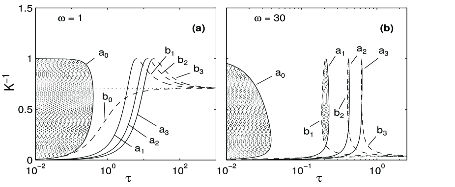
FIG. 1.: The stability of the origin is shown in a $(\tau,K^{-1})$ diagram for (a) $\omega=1,a=1$ and (b) $\omega=30,a=1$. At lower values of $\omega$ there is only one death region that is confined between $\tau=0$ and $\tau=\tau_{1}(0,K)$, but for higher values of $\omega$ there are generally multiply connected regions of amplitude death. The curves $a_{n}$ and $b_{n}$ represent $\tau_{1}(n,K)$ and $\tau_{2}(n,K)$ respectively. The dotted horizontal line is $1/f(\omega)$.

To obtain the critical curves, set $\alpha=0$. This gives

$$\beta|_{\alpha=0}=\omega\pm\sqrt{K^{2}-a^{2}}.$$ (9)

By inverting Eq. (5), and noting that $\sin(\beta_{+}\tau)>0$, $\sin(\beta_{-}\tau)<0$, and that $\beta_{-}$ can be either positive or negative, we obtain the following two sets of critical curves:

$$\tau_{1}(n,K)=\frac{2n\pi+\cos^{-1}(a/K)}{\omega+\sqrt{K^{2}-a^{2}}},$$ (10)

$$\tau_{2}(n,K)=\frac{2n\pi-\cos^{-1}(a/K)}{\omega-\sqrt{K^{2}-a^{2}}}.$$ (11)

In Eq. (10), $n=0,1,2,\ldots$. In Eq. (11), if $\beta_{-}>0,~{}n=1,2,\ldots$; if $\beta_{-}<0,~{}n=0,1,2,\ldots$. Thus the critical curves exist only in the region $K\geq a$. Since, for $\tau=0$, the region of stability of the origin is given by $K>a$, the corresponding region, for $\tau>0$, will be given by the area between $\tau=0$ and the critical curve closest to the line $\tau=0$. This critical curve should be the one on which $d\alpha/d\tau>0$. From (4)

$$\frac{d\lambda}{d\tau}=\frac{K\lambda e^{-\lambda\tau}}{1-K\tau e^{-\lambda\tau}}~{}~{},$$ (12)

and

$$\frac{d\alpha}{d\tau}\Bigg{|}_{\alpha=0}=\mathrm{Re}\frac{K(i\beta)e^{-i\beta\tau}}{1-K\tau e^{-i\beta\tau}} = \beta~{}K\sin(\beta\tau)~{}D^{-1}$$ (13)

$$= \beta(\beta-\omega)~{}D^{-1},$$ (14)

where $D=[1-K\tau\cos(\beta\tau)]^{2}+[K\tau\sin(\beta\tau)]^{2}$ is positive real. Hence

$${\frac{d\alpha}{d\tau}}\Bigg{|}_{\alpha=0}\cases{>0&on $\tau_{1}$,\cr>0&on $\tau_{2}$ if $K>f(\omega)$,\cr=0&on $\tau_{2}$ if $K=f(\omega)$,\cr<0&on $\tau_{2}$ if $K<f(\omega)$,\cr}$$ (15)

where $f(\omega)=\sqrt{a^{2}+\omega^{2}}$. The above condition implies that there can be only one stability region if $K>f(\omega)$. There is a possibility of multiple stability regions if $K<f(\omega)$. Our numerical plot in Fig. 1(a) of the curves $\tau_{1}(n,K)$ and $\tau_{2}(n,K)$ reveals that the region between $\tau=0$ and $\tau=\tau_{1}(0,K)$ is the only stability region possible for small values of $\omega$. However, as the value of $\omega$ is increased, the stability regions can be specified by $0\leq\tau<\tau_{1}(0,K)$ and $\tau_{2}(n,K)<\tau<\tau_{1}(n,K)$, where $n>0$. In Fig. 1(b) the critical curves are plotted from Eqs. (10) and (11) for such a large value of $\omega$, namely $\omega=30$, and the multiple stability regions are represented by the shaded portions. Note that a similar situation arises in the case of two or more limit cycle oscillators that are coupled by a time delay. This was investigated in detail in [23, 24], where the collective stability regions were termed amplitude death regions or death islands in the $K-\tau$ space.

We conclude this section by carrying out a stability analysis of the origin in the $(a,K)$ plane for a fixed value of $\tau$. Using Eqs.(5-6) we write below the critical curves which are non intersecting:

$$K(\beta)=\frac{\beta\pm\omega}{\sin(\beta\tau)},~{}~{}and~{}~{}a(\beta)=\frac{\beta\pm\omega}{\sin(\beta\tau)}~{}\cos(\beta\tau).$$ (16)

We note that the above expressions for $K(\beta)$ and $a(\beta)$ have singularities at $\beta=n\pi/\tau$ and between any two successive singular points the expressions produce continuous curves in $(a,K)$ plane. Following Diekmann et al. [40], we define the following intervals where the sign of the superscript of $I$ indicates the sign of the function $\sin(\beta\tau)$ in that interval:

$$I^{-}_{n}=\left((2n-1)\frac{\pi}{\tau},~{}2n\frac{\pi}{\tau}\right),~{}~{}~{}I^{+}_{n}=\left(2n\frac{\pi}{\tau},~{}(2n+1)\frac{\pi}{\tau}\right),$$ (17)

for $n=0,1,2,\ldots.$ We restrict our attention, without loss of generality, to the case of $\beta\geq 0$. Hence we can define the following curves in $(a,K)$ plane.

$$C^{\pm}_{n}=\Bigg{\{}(a,K)=\Bigg{(}\frac{(\beta-\omega)~{}\cos(\beta\tau)}{\sin(\beta\tau)},~{}\frac{(\beta-\omega)}{\sin(\beta\tau)}\Bigg{)}~{}\Bigg{|}~{}\beta\in I^{\pm}_{n}\Bigg{\}},$$ (18)

$$D^{\pm}_{n}=\Bigg{\{}(a,K)=\Bigg{(}\frac{(\beta+\omega)~{}\cos(\beta\tau)}{\sin(\beta\tau)},~{}\frac{(\beta+\omega)}{\sin(\beta\tau)}\Bigg{)}~{}\Bigg{|}~{}\beta\in I^{\pm}_{n}\Bigg{\}}$$ (19)

These curves are parametrized by $\beta$. The curves are degenerate at $\omega=n\pi/\tau$. For $\omega=2n\pi/\tau,~{}~{}n=0,1,2,\ldots$, both the curves $C_{n}^{\pm}$ and $D_{n}^{\pm}$ merge, and there is another curve in addition to the above, defined by

$$C_{R}=\{(K,a)~{}\mid~{}a=K\}$$ (20)

with $\beta=2n\pi/\tau$. Likewise for $\omega=(2n+1)\pi/\tau,~{}~{}n=0,1,2,\ldots$, the corresponding additional curve is defined by

$$C_{R}=\{(K,a)~{}\mid~{}a=-K\}$$ (21)

with $\beta=(2n+1)\pi/\tau$. We are now only left with the task of finding out the number of the eigenvalues in the right half plane on either side of the curves $C_{n}^{\pm}$ and $D_{n}^{\pm}$. For our particular problem it is possible to carry out this analysis in an exact manner. Let $F(a,K,\lambda)=\lambda-a\mp i\omega+Ke^{-\lambda\tau}=0$ be the eigenvalue equation. Define $G_{1}=$Re$F$, $G_{2}=$ Im $F$, and at $\alpha=0$ define a matrix $M$ by

$$M=\left(\matrix{\frac{\partial G_{1}}{\partial a}&\frac{\partial G_{1}}{\partial K}\cr\cr\frac{\partial G_{2}}{\partial a}&\frac{\partial G_{2}}{\partial K}}\right).$$ (22)

We now make use of a proposition of Diekmann et al. [40] to determine the positions of the eigenvalues in the complex plane with respect to the curves $(a(\beta),K(\beta))$. The proposition states that the critical roots are in the right half-plane in the parameter region to the left of the curve $(a(\beta),K(\beta))$, when we follow this curve in the direction of increasing $\beta$, whenever $\det M<0$ and to the right when $\det M>0$. In the present case, on both the curves $C^{\pm}_{n}$ and $D^{\pm}_{n}$, the matrix is given by

$$M=\left(\matrix{-1&\cos(\beta\tau)\cr\cr 0&-\sin(\beta\tau)}\right),$$ (23)

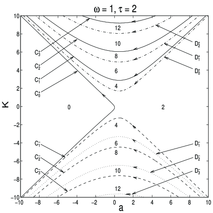
FIG. 2.: Critical curves in (a,K) plane. The numbers indicate the number of eigenvalues in the right half plane of the complex eigenvalue space. The amplitude death region is the region where there are zero eigenvalues in the right half plane. The arrow on each curve shows the direction along which $\beta$ increases.

and hence $\det(M)=\sin(\beta\tau)$. It is easily seen that $\det M>0$ on $C_{n}^{+}$, $D_{n}^{+}$, and $\det M<0$ on $C_{n}^{-}$, $D_{n}^{-}$. And finally we know that the stability region for $\tau=0$ is given by $a<K$. Combining these facts we present our results for the stability region and the number of eigenvalues in Fig. 2. The amplitude death region is the region where there are no (i.e. zero) eigenvalues in the right half plane.

B Periodic Solutions

We now examine the region where the origin is unstable. For $\tau=0$ this region sustains periodic solutions as discussed in the introductory remarks of this section. We now look for periodic solutions in the presence of time delay. For this, it is convenient to cast Eq. (3) in polar form. For simplicity, we also set $a=1$ implying that the oscillator without any kind of feedback has a unit circle as its periodic solution, and the phase increases linearly on the circle. Writing Eq. (3) in polar coordinates we have,

$$\dot{r}(t)=[1-r^{2}(t)]r(t)-Kr(t-\tau)~{}\cos[\theta(t-\tau)-\theta(t)],$$ (24)

$$\dot{\theta}(t)=\omega-K\frac{r(t-\tau)}{r(t)}~{}\sin[\theta(t-\tau)-\theta(t)].$$ (25)

Recall that when $\tau=0$, Eq. (3) has the time asymptotic periodic solution $Z(t)=\sqrt{1-K}~{}e^{i\omega t}$. For non zero $\tau$ we can still assume a periodic solution of the form $Z(t)=R~{}e^{i\Omega t}$; i.e., we are looking for solutions of the form $r(t)=R$ and $\theta(t)=\Omega t$, where $R$ and $\Omega$ are real constants. In fact, it can be checked that this is the only solution which has a linear growth of the phase. Substituting this form in Eqs. (24) and (25) and after some algebra, we obtain the following relations for the amplitude and the frequency of the oscillator:

$$R =\sqrt{1-K~{}\cos(\Omega\tau)},$$ (26)

$$\Omega =\omega+K~{}\sin(\Omega\tau).$$ (27)

The oscillator can now lie outside the unit circle when $\cos(\Omega\tau)<0$; that is, the amplitude of the limit cycle can increase beyond unity if $\tau\in((2n+\frac{1}{2})\pi/\Omega,(2n+\frac{3}{2})\pi/\Omega)$. However, the amplitude is bounded for any value of $\tau$ because $max(R)\leq\sqrt{1+K}$. So for any given $K$, the amplitude of the limit cycle stays in the interval $[\sqrt{1-K},\sqrt{1+K}]$ for arbitrary values of $\tau$. The above condition on $\Omega\tau$ can be used in Eq. (27) to infer bounds on the frequency of the limit cycle: $\omega-K\leq\Omega\leq\omega+K$.

Eq. (27) admits multiple solutions for the frequency $\Omega$. The left-hand side, $y_{1}=\Omega$, of (27) is a straight line and the right-hand side, $y_{2}=\omega+K~{}\sin(\Omega\tau)$, is a sinusoidal curve with amplitude $K$ and a shift of $\omega$ above the horizontal axis, $y=0$. The multiple solutions (frequencies) are given by the intersection of the curves $y_{1}$ and $y_{2}$. As the value of $K$ is increased for a fixed value of $\omega$, the curve $y_{2}$ makes more and more intersections with $y_{1}$ and thus a set of multiple frequencies comes into existence. Similarly a variation in $\omega$ will also bring about changes in the number of possible solutions. But for all values of $\omega$, including for $\omega=0$, multiple frequency solutions are possible. The existence of multiple frequencies is a characteristic feature of time delay systems and has been noted before in the context of the Kuramoto model with time delay [20] and in other studies [19, 23, 25]. These multiple frequency states that coexist with the lowest frequency state can be accessed by a suitable choice of initial conditions and have potential applications in coupled oscillator models of the human brain.

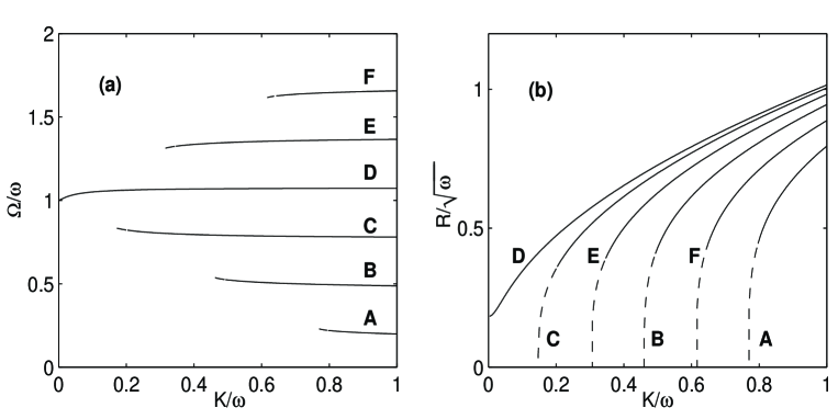
FIG. 3.: Finite time delay leads to the existence of multiple periodic states, which can coexist with the primary limit cycle state. The frequencies and amplitudes of these states (for $\tau=0.68$) are plotted as a function of the coupling strength $K$ in (a) and (b) respectively. As the value of the strength of the feedback, $K$, is increased, the number of periodic orbits increases. In both the plots the dashed portions of the curves are unstable regions.

In Fig. 3(a) we plot these multiple frequencies, $\Omega$, for $\omega=30$ and $f=3.25$ where $f=\omega\tau/(2\pi)$. Fig. 3(b) shows the corresponding amplitudes of the multiple states. Some of these states merge if $f$ is an integer. This can be inferred from the intersections of the amplitude curves in Fig. 3(b). At these points, the oscillator has two frequencies with a single amplitude. To find out these frequencies, let $\Omega_{1}$ and $\Omega_{2}$ be the two frequencies at these degenerate points. Substituting these values in the expression for $R$ in (26), we get $\frac{\Omega_{1}}{\omega}=\frac{\Omega_{2}}{\omega}+\frac{m}{f}$, where $m$ is an integer.

Stability of the Multiple States. The stability of these multiple periodic solutions can be obtained by linearizing about each of the solutions. The linearized matrix of Eqs. (24) and (25) about the periodic solutions can be written as

$$M_{1}~{}=~{}\left[\matrix{A-Be^{-\lambda\tau}&RC(1-e^{-\lambda\tau})\cr-\frac{C}{R}(1-e^{-\lambda\tau})&B(1-e^{-\lambda\tau})}\right],$$

where $A=1-3R^{2},$ $B=K~{}\cos(\Omega\tau),$ and $C=K~{}\sin(\Omega\tau)$. The corresponding eigenvalue equation is $\det(M_{1}-\lambda I)=0$, or

$$A_{1}e^{-2\lambda\tau}-A_{2}e^{-\lambda\tau}+A_{3}+\lambda^{2}-A_{4}\lambda+A_{5}\lambda e^{-\lambda\tau}=0,$$

where $A_{1}=B^{2}+C^{2}$, $A_{2}=AB+B^{2}-2C^{2}$, $A_{3}=AB+C^{2}$, $A_{4}=A+B$ and $A_{5}=2B$. If $\tau=0$, then $\lambda=\{0,-2(1-K)\}$. We thus recover the result that the periodic solution is stable for $\tau=0$ when $K<1$. For $\tau\neq 0$ we need to solve the eigenvalue equation numerically. Our numerical results for the stability of the multiple periodic states are incorporated in Fig. 3 and Fig. 4 where the dashed portions of the curves indicate unstable regions. At large value of $\tau$, the frequency of the oscillation , $\Omega$, gets reduced. This is true for all the multiple frequency states that the system possesses. In Fig. 4(a) the normalized frequency of each of the states is plotted against the time delay on a log scale. The frequencies are suppressed at a rate proportional to $\tau^{-1}$. Fig. 4(b) shows the corresponding amplitudes plotted against time delay. This feature of frequency suppression has been observed in the past for large coupled systems [20] and once again seems to have its roots in the behavior of a single oscillator in the presence of a time delayed feedback drive. However, for short time delays, as may be seen from the figures, the effect of time delay is some what distinct - both the frequency and the amplitude of the oscillator increase slightly with $\tau$. To understand this behavior we present in Section II C analytic expressions for the time evolution of $Z(t)$ in the limit of small time delay.

C Small $\tau$ approximation

For short time delays, it is still worthwhile to expand the delay variable $Z(t-\tau)$ in a Taylor series despite occasional warnings [41]. Let us write

$$Z(t-\tau)=Z(t)-\tau\dot{Z}(t)+\frac{\tau^{2}}{2}\ddot{Z}(t)\ldots$$

Substituting in Eq. (3), the following two equations for the first two orders can be written.

$$O(\tau):~{}~{}$$ (31)

$$\dot{Z}(t)=\left[(1+i\omega-\mid Z(t)\mid^{2})Z(t)-KZ(t)\right]\Big{/}(1-K\tau),$$

$$O(\tau^{2}):~{}~{}$$

$$\ddot{Z}(t)+b\dot{Z}(t)-c(1-K+i\omega-\mid Z(t)\mid^{2})Z(t)=0,$$

where $b=2(1-K\tau)/K\tau^{2}$ and $c=2/K\tau^{2}$. It can be checked easily that the asymptotic periodic solutions are given by

$$O(\tau):~{}~{} Z(t)=\sqrt{1-K}~{}e^{i\omega^{\prime}t},$$ (32)

$$O(\tau^{2}):~{}~{} Z(t)=\left[1-K+\frac{\omega^{2}K\tau^{2}}{2(1-K\tau)^{2}}\right]^{1/2}~{}e^{i\omega^{\prime}t},$$ (33)

where $\omega^{\prime}=\omega/(1-K\tau)$. The effect of small $\tau$ is evident on the frequency and the amplitude: both show a slight rise.

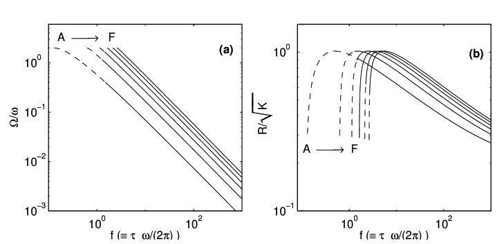
FIG. 4.: The frequencies and amplitudes of the multiple periodic states are plotted as a function of $f=\tau\omega/(2\pi)$ in (a) and (b) respectively at $K=\omega=30$. At large values of $\tau$, the frequency suppression is algebraic and is proportional to $1/\tau$. In both the plots the unstable portions are indicated by dashed lines.

III Nonlinear Feedback Effects

In this section we include the nonlinear feedback term ($K_{2}\neq 0$) and examine the dynamics of the limit cycle oscillator in the presence of the complete feedback term $f$ as given in (2). We then have

$$\dot{Z}(t)=(a+i\omega-\mid Z(t)\mid^{2})Z(t) - K_{1}Z(t-\tau)$$ (34)

$$- K_{2}Z^{2}(t-\tau).$$ (35)

The transformations $Z(t)\rightarrow e^{i\pi}Z(t)$ and $K_{2}\rightarrow-K_{2}$ leave the equation unchanged. The bifurcation diagrams, thus, appear symmetric about $K_{2}=0$ axis with the exception that the orbits are rotated by an angle of $\pi$ about the origin.

A $\tau=0$

In order to distinguish the additional effects arising from the nonlinear feedback term we first turn-off the time delay and examine the dynamics for $\tau=0$. These solutions also correspond to the special class of solutions with time delay when the solutions have a periodic recurrence with a period $\tau$. These are generally termed as phase trapped solutions in the literature. Let $Z=X+iY$. The evolution equations are

$$\dot{X} = (a-X^{2}-Y^{2})X-\omega Y-K_{1}X-K_{2}(X^{2}-Y^{2}),$$ (36)

$$\dot{Y} = \omega X+(a-X^{2}-Y^{2})Y-K_{1}Y-2K_{2}XY.$$ (37)

1 Fixed points

The fixed points of the system are found by solving $\dot{X}=0$ and $\dot{Y}=0$ simultaneously. In contrast to the earlier case of a linear feedback drive, there are now three fixed points of the system including the origin. In Table 1, the fixed points and expressions for the eigenvalues of linear perturbations around these fixed points are listed using the definitions TABLE I.: Symbol index Fixed point Eigenvalues j $(X_{j}^{*},Y_{j}^{*})$ $\lambda$ $D$ 0 $(0,0)$ $-\tilde{K}_{1}~{}\pm~{}i\omega$ $FP_{1}$ 1 $(-\frac{K_{2}}{2}+\sqrt{G},\frac{\omega}{K_{2}})$ $\tilde{K_{1}}~{}\pm~{}T_{1}$ $FP_{2}$ 2 $(-\frac{K_{2}}{2}-\sqrt{G},\frac{\omega}{K_{2}})$ $\tilde{K_{1}}~{}\pm~{}T_{2}$

$G=(\frac{K_{2}}{2})^{2}-\tilde{K_{1}}-\frac{\omega^{2}}{K_{2}^{2}}$, $\tilde{K}_{1}=K_{1}-a$ and $T_{i}=\sqrt{({X_{i}^{*}}^{2}+{Y_{i}^{*}}^{2})^{2}-\omega^{2}}$. As can be seen, the origin exists as a fixed point for all the values of the parameters $K_{1},K_{2},a$ and $\omega$. However, it is stable only when $\tilde{K}_{1}>0$, i.e. when $K_{1}>a$. The other two fixed points $FP_{1}$ and $FP_{2}$ exist in the region where $G>0$. This condition gives rise to $K_{2}>\gamma(\tilde{K}_{1})$ and $K_{2}<-\gamma(\tilde{K}_{1})$, where $\gamma(\tilde{K}_{1})\equiv\sqrt{2}\sqrt{\tilde{K}_{1}+\sqrt{\tilde{K}_{1}^{2}+\omega^{2}}}$. This region overlaps with $\tilde{K}_{1}>0$. Fig. 5 shows the bifurcation diagram. The regions marked with $D$, $FP_{1}$ and $FP_{2}$ are the regions in which the corresponding fixed points are stable. The region $D$ is bounded on the right hand side by $K_{1}=a$. The region $FP_{1}$ is bounded by the curves $\tilde{K}_{1}=0$ and $K_{2}=\gamma(\tilde{K}_{1})$. The region $FP_{2}$ is bounded by the curves $\tilde{K}_{1}=0$ and $K_{2}=-\gamma(\tilde{K}_{1})$. The movement of these fixed points and the corresponding eigenvalues are shown in Fig. 6.

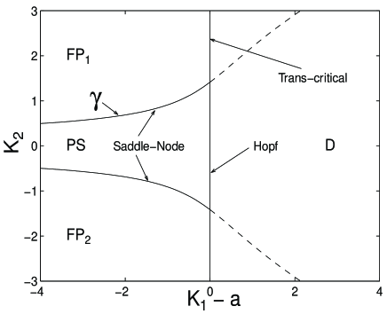
FIG. 5.: The bifurcation diagram of Eq. (34) for $\tau=0$ in $(\tilde{K}_{1},K_{2})$ plane for $a=1$, $\omega=1$. $D$ is the region of amplitude death, $FP_{1}$ and $FP_{2}$ are the regions of stability of the fixed points $FP_{1}$ and $FP_{2}$ respectively. The periodic solution is stable in the region $PS$.

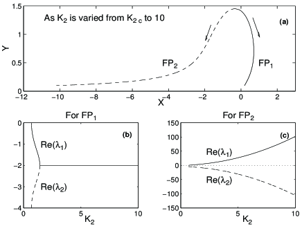
FIG. 6.: The movement of the fixed points of Eq. (34) for $\tau=0$ ($K_{1}=-1$, $a=1$, and $\omega=1$) is shown in (a) as $K_{2}$ is varied from the critical value $K_{2c}=0.6871$ to $10$. The behavior of the real parts of the eigenvalues for the corresponding fixed points are plotted in (b) and (c) respectively and show that $FP_{1}$ is stable and $FP_{2}$ is unstable in this case.

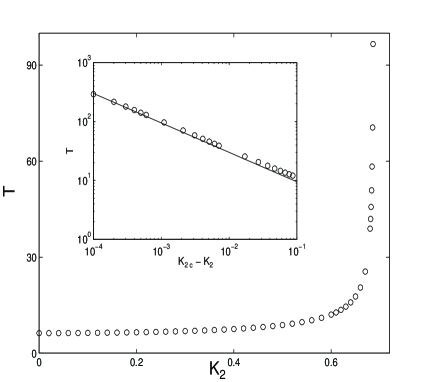
FIG. 7.: The variation of the period of the limit cycle in the region $PS$ of Fig. 5. as a function of $K_{2}$ for a fixed value of $K_{1}=-1$. As $K_{2}$ is increased from $0$ to $\gamma(K_{1})$ the period increases from $2\pi/\omega$ to infinity with a scaling proportional to $1/\sqrt{(K_{2c}-K_{2})}$ and leading to a saddle-node bifurcation. The inset displays on a log scale the behavior close to the critical region. The solid curve is a plot of $3/\sqrt{K_{2c}-K_{2}}$.

2 Periodic orbit

Eqs. (36) and (37) have a stable periodic solution in the region $-\gamma(K_{1})<K_{2}<\gamma(K_{1})$. The periodic orbit develops a saddle $(FP_{2})$ and a node $(FP_{1})$ as $K_{2}$ is increased above $\gamma(K_{1})$. Similarly as $K_{2}$ is decreased below $-\gamma(K_{1})$ a node $(FP_{2})$ and a saddle $(FP_{1})$ are born. The periodic orbit is a circle for $K_{2}=0$ and the oscillator moves linearly on the circle with a frequency $\omega$. As $K_{2}$ is increased or decreased the period of the limit cycle increases and tends to infinity on the curve $K_{2}=\pm\gamma(\tilde{K}_{1})$ giving birth to a saddle-node point. In Fig. 7 we have plotted the period of the limit cycle as a function of $K_{2}$ for $K_{1}=-1,a=1,\omega=1$. The inset of this figure also shows the scaling of the approach to infinite time period which in this case is the typical inverse square root scaling of the saddle-node bifurcation phenomenon. As can be seen from Table 1, one of the eigenvalues of the Jacobian of Eqs. (36) and (37) is zero at the critical value of $K_{2}$. The existence of the saddle-node bifurcation can thus be rigorously established by reducing the dynamics to the center manifold [46].

Phase slips. As the magnitude of $K_{2}$ is increased from $0$ to $\pm\gamma(K_{1})$ the evolution of the phase of the oscillator takes on a nonlinear character. The parabolic nature of $\dot{\theta}(\theta)$ at its minimum and its sinusoidal nature for other values of $\theta$ indicate the existence of a nonuniform motion of the oscillator from $0$ to $2\pi$. The motion becomes jerky as the parameter is increased to bring a tangency at which point $\dot{\theta}=0$. The time period becomes singular at the point of tangency.

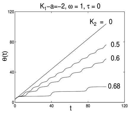
FIG. 8.: Phase slips of the limit cycle oscillator for $\tau=0,K_{1}=-1,a=1,\omega=1$. The phase of the limit cycle oscillator evolves linearly on the circle when there is no nonlinear feedback. With increasing $K_{2}$ one clearly sees the phase slips suffered by the oscillator.

It begins to spend more and more time in the vicinity of $\theta=\theta^{*}$ and less and less time at other values. Close to the curves $\pm\gamma(K_{1})$ the oscillator shows clear phase slips of $2\pi$ as seen in Fig. 8. This phase slip ends with phase quenching on the boundary of $\pm\gamma(K_{1})$. In this state the phase of the oscillator is a constant and such a state is often referred to as phase death. The phenomenon of phase slips plays an important role in the process of transition towards a synchronized state in a system of a large number of coupled limit cycle oscillators and has been the subject of some recent investigations [43].

B $\tau>0$

We now return to our full feedback model and include the effect of finite time delay on the dynamical characteristics of the oscillator. Since we now have an infinite dimensional system, the phase space dynamics can in general be quite complicated and changes significantly as a function of the time delay parameter $\tau$. For our further analysis and description, we write down the Eq. (34) in polar coordinates.

$$\dot{r}(t) = [a-r^{2}(t)]r(t)-K_{1}r(t-\tau)\cos[\theta(t-\tau)-\theta(t)]$$ (39)

$$\hskip 28.45274pt-K_{2}r^{2}(t-\tau)~{}\cos[2\theta(t-\tau)-\theta(t)],$$

$$\dot{\theta}(t) = \omega-K_{1}\frac{r(t-\tau)}{r(t)}\sin[\theta(t-\tau)-\theta(t)]$$ (41)

$$\hskip 28.45274pt-K_{2}\frac{r^{2}(t-\tau)}{r(t)}~{}\sin[2\theta(t-\tau)-\theta(t)].$$

FIG. 9.: Bifurcation diagram of Eq. (34) for $\tau=0.5$, $a=1$, $\omega=1$. The areas marked $FP_{1}$ and $FP_{2}$ refer to stability domains of these fixed points, the region $W-1$ sustains limit cycle orbits encircling the origin (winding number 1), the regions $BS_{1},BS_{2}$ contain combinations of phase reversing, radially trapped or spiraling solutions in a birythmic existence, and the regions marked $CR-I,CR-II,CR-III,CR-IV$ exhibit chaotic behavior interspersed with periodic windows.

In the following we describe several different solutions which are found numerically (depicted in Fig. 9 and the following figures) and provide explanation in terms of the behavior of the amplitude and the phase. These solutions include birhythmicity, phase reversals, phase slips, radially trapped orbits, phase jumps, and spiraling orbits. For all the numerical integrations, unless stated otherwise, we use a constant history function: $Z(t)=Z(0),~{}t\in[-\tau,0)$ and a constant step size (h) of integration. Several values of $h$ were tested for the accuracy of the results. Issues relating to the numerical integration of delay differential equations can be found in [44]. In all our later results we set the parameters $a=1$ and $\omega=1$.

Before we begin our description of the solutions to Eqs. (39) and (41), we wish to point out an important connection between the present model and some of the other models that have been studied in the literature. Under the assumptions that $K_{1}=0$, $\mid\theta(t-\tau)-\theta(t)\mid<<1$, and $r(t)=r(t-\tau)=1$, Eq. (41) yields

$$\dot{\theta}(t)=\omega - K_{2}~{}\sin\theta(t-\tau)$$ (42)

$$- K_{2}~{}[\theta(t-\tau)-\theta(t)]~{}\cos\theta(t-\tau).$$ (43)

The above equation with the first two terms on the right hand side describes a first order phase locked loop with time delay [30]. It also has the structure of the equation that can be used to model certain visually guided movements of biological limbs [32].

1 Stability of the fixed points

We proceed first to carry out a linear perturbation analysis of Eq. (34) around the three fixed points and then construct the bifurcation diagram for fixed values of $\tau$ through detailed numerical investigations. The analysis of the stability of the origin remains unchanged by the presence of the $K_{2}$ term since its contribution vanishes in the linear limit. So its behavior can be discerned from the previous section (e.g. see Fig. 1(a)), where we saw that the amplitude death region shrinks and moves to the right of the curve $\tilde{K}_{1}=0$ as $\tau$ is increased from $0$ and vanishes at a certain critical value. Depending on the strength of $\omega$, it may reappear. For the present study we choose $\omega=1$ and $\tau=0.5$, which is much less than the intrinsic time period $2\pi$. For this value the amplitude death region disappears and the origin is always unstable. The fixed points $FP_{1}$ and $FP_{2}$ are again the same as discussed in the previous section, but their stability properties are now significantly modified due to finite time delay effects. Let $Z^{*}=(X^{*}+iY^{*})$ be one of the non-zero fixed points of the system. A linearization about $Z^{*}$ of (34) yields

$$\dot{z}(t)=(a+i\omega-2\mid Z^{*}\mid^{2})z(t)$$ (44)

$$\hskip 56.9055pt-{Z^{*}}^{2}\bar{z}(t)-(K_{1}+2K_{2}Z^{*})z(t-\tau),$$ (45)

where $z=Z-Z^{*}$ and $\bar{z}$ is the complex conjugate of $z$. Write $z(t)=x(t)+iy(t)$ and assume each component to vary as $e^{\lambda t}$, where $\lambda$ is the eigenvalue of the linearized matrix, $M_{2}$, whose eigenvalue equation is given by $\det(M_{2}-\lambda I)=0$, and can be written as

$$(A-Be^{-\lambda\tau}-\lambda)^{2}-2({X^{*}}^{2}+{Y^{*}}^{2})(A-Be^{-\lambda\tau}-\lambda)$$ (46)

$$+(2K_{2}Y^{*}e^{-\lambda\tau}-\omega)^{2}=0,$$ (47)

where $A=a-({X^{*}}^{2}+{Y^{*}}^{2})$ and $B=K_{1}+2K_{2}X^{*}$. The evolution of $\lambda$ in the complex plane as $K_{1}$ and $K_{2}$ are varied decides the stability of the fixed points. The relation between $K_{1}$ and $K_{2}$ for the critical boundary is not very transparent from the above equation. We use Eq. (47) to determine the boundaries of the regions of these fixed points numerically and present the bifurcation diagram in Fig. 9. The regions labelled $FP_{1}$ and $FP_{2}$ represent the regions of stability of the respective fixed points. When $K_{2}$ is small and one is in the region where the origin is unstable but $FP_{1}$ and $FP_{2}$ are stable, the limit cycle orbit preserves its identity and the results are similar to those discussed in earlier sections. As $K_{2}$ is increased in magnitude, however, several interesting new orbits depicted in the bifurcation diagram appear. We discuss these features below.

2 Periodic solution

The simple periodic orbit (limit cycle) exists for all small values of $K_{2}$ in the region marked as W-1 in Fig. 9. As $K_{2}$ is increased this stability can be lost through a variety of bifurcations (e.g. saddle node bifurcation, bistability or chaos). The most interesting effect of a finite delay time appears to be on the nature of the saddle-node bifurcation. Although the period of the limit cycle becomes infinite at the bifurcation point, the scaling behavior and the nature of the orbit dynamics near this point are significantly different from those of the $\tau=0$ case. To illustrate this point, we have plotted in Fig. 10(a) a set of $\dot{\theta}$ vs. $\theta$ curves for $\tau=0.3,K_{1}=0$ as $K_{2}$ is successively increased towards the critical value. Note that the nature of the $\dot{\theta}$ curve is not parabolic near the critical point and has distinct asymmetries. Further, $d\dot{\theta}/d\theta$ develops a discontinuity at this point as shown in Fig. 10(b). Since $\dot{\theta}$ goes to $0$ near the critical point, the period of the limit cycle keeps increasing as $K_{2}$ approaches the critical value as shown in Fig. 10(c). The discontinuity of $d\dot{\theta}/d\theta$ is a significant deviation from the standard conditions of a saddle-node bifurcation [46] and brings about the change in the scaling behavior. To analytically estimate the time period close to the bifurcating point, the $\dot{\theta}$ curve, in the vicinity of the critical point, can be approximated as

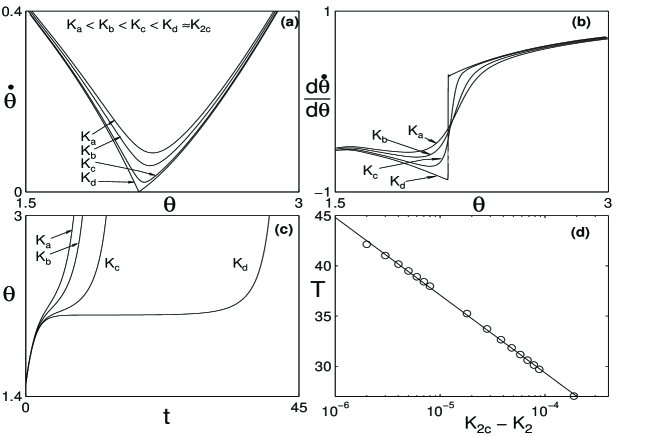
FIG. 10.: The nature of (a) $\dot{\theta}$ and (b) $d\dot{\theta}/d\theta$ as a function of $\theta$ close to the bifurcation point, and (c) the corresponding stretching of the time period of the periodic orbit. (d) A semilog plot of the numerically obtained time periods $T$ vs. $(K_{2c}-K_{2})$ (shown as circles) which indicates a logarithmic scaling of the singularity, viz. $T=-3.3665\log(K_{2c}-K_{2})-1.6772$ (solid line). Here $K_{2c}=0.923488$, $K_{1}=0$, $a=1$, $\omega=1$ and $\tau=0.3$.

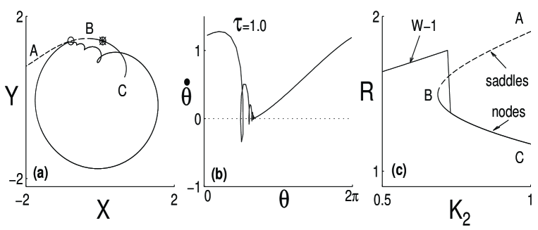
FIG. 11.: Periodic orbit losing stability by colliding with the saddle. (a) periodic orbit just before the critical value of $K_{2}$, (b) corresponding evoluation of $\dot{\theta}$ as a function of $\theta$. (c) shows the bifurcation diagram as $K_{2}$ is increased. $R$ is the maximum value of the asymptotic state of the oscillator. The parameters are $\tau=1.0,K_{1}=-1,a=1$, and $\omega=1$.

$$\dot{x}=\cases{-b_{1}x+c_{1},&if $x<0$\cr b_{2}x+c_{1},&if $x>0$}$$ (48)

where $x=\theta-\theta^{*}$, $\dot{\theta}$ is minimum at $\theta^{*}$ for a given value of $K_{2}$, and $b_{1},b_{2}$ and $c_{1}$ are all positive constants. ($c_{1}=0$ when $K_{2}=K_{2c}$). The time period across a thin region $2\delta$ around $x=0$ is now given by

$$T \approx \int_{-\delta}^{0}\frac{dx}{-b_{1}x+c_{1}}+\int_{0}^{\delta}{\frac{dx}{b_{2}x+c_{1}}}$$ (49)

$$= -\Big{(}\frac{1}{b_{1}}+\frac{1}{b_{2}}\Big{)}\log c_{1}$$ (51)

$$\hskip 28.45274pt+\log\Big{(}(b_{1}\delta+c_{1})^{1/b_{1}}(b_{2}\delta+c_{1})^{1/b_{2}}\Big{)}$$

As seen from the first term in the expression above, the time period goes to infinity as $c_{1}\to 0$ with a logarithmic scale. This is in contrast to the inverse square root scaling for the $\tau=0$ case. The above scaling agrees quite well with our numerical results as shown in Fig. 10(d). The actual mechanism of the loss of stability of the periodic orbit is through a collision with the saddle point. This is illustrated in Fig. 11 which is plotted for $K_{1}=-1$ and $\tau=1.0$. The curves BC and BA are the stable ($FP_{1}$) and unstable ($FP_{2}$) branches, and they are the same as those depicted in Fig. 6(a). As seen in the $(X,Y)$ plane in Fig. 11(a), the orbit collides with an existing saddle point and is kicked to the stable node. Fig. 11(b) shows the corresponding behavior of $\dot{\theta}$ vs. $\theta$ just before the critical value of $K_{2}$. Notice that its intersection with the $\dot{\theta}=0$ line is non-parabolic. There are also additional intersections which however are not fixed points since $\dot{r}\neq 0$ at these points. These loops have significance for the phase reversal orbits which we discuss in Section III B 3. In Fig. 11(c), $R$ is the maximum amplitude of the asymptotic state of the orbit at each $K_{2}$.

3 Phase reversals

While still inside the region W-1, the periodic orbit can show a reversal of its phase with time with the same period as that of the orbit; the curve $\dot{\theta}(\theta)$ develops a fold as $K_{2}$ is increased. Depending on the value of $K_{1}$ there can be one or more than one folds. The acquired additional loop as shown in Fig. 12(a) is not around the origin; the winding number of the periodic orbit continues to be one. However the phase of the orbit as measured from the origin undergoes a reversal in that region (Fig. 12(b)), in contrast with the phase slip behavior discussed earlier. This is purely the effect of the time delay appearing in the nonlinear feedback term. The phase reversing orbits are prominent at the boundaries of the W-1 region. Such periodic orbits for a single oscillator have been observed for externally driven systems and basically arise due to the excitation of higher harmonics from the resonant interaction of the external driver with the basic oscillator [45]. They cannot exist for a single autonomous oscillator in the absence of time delay due to dimensional constraints. However the presence of time delay in our autonomous model increases the dimensionality of the system and hence permits the existence of such orbits. This is a new kind of orbit which does not seem to have been noticed or discussed before in the context of large systems of coupled oscillators and it would be worthwhile looking for their existence in such systems.

4 Effect of time delay on phase slips

The phenomenon of phase slips continues to exist for non zero values of time delay as well. To study the effect of time delay on the phase slips, we examine Fig. 8 and choose the parametric values corresponding to the phase slips shown by the bottom most curve, i.e. for $K_{2}=0.68$, and introduce finite time delay. The results are shown in Fig. 13. Time delay has the effect of reducing the sharpness of the phase slips and, at the same time, increasing the angular speed as seen by the slope of $\theta$. For longer time delays, (e.g. for $\tau=2.0$ in the figure), phase slips are less evident and in fact the orbits exhibit chaos.

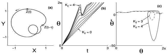
FIG. 12.: Phase reversal. (a) A phase reversing orbit of the limit cycle in the $X-Y$ space for $K_{2}=4.0$. (b) Temporal evolution of the phase as measured from the origin as a function of $K_{2}$ as $K_{2}$ is increased from $0$ to $4$ in steps of $0.5$. (c) The multivaluedness of $\dot{\theta}(\theta)$. The other constants are $K_{1}=1.4,a=1,\omega=1$, and $\tau=0.5$.

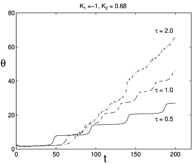
FIG. 13.: The effect of time delay on phase slips. ($K_{2}=0.68$, $K_{1}=-1,a=1$, and $\omega=1$.)

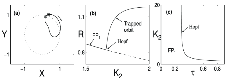
FIG. 14.: Radial trapping. (a) A radially trapped orbit of the limit cycle in the $X-Y$ space. $\star$ and $\circ$ show two points separated in time by $\tau$. (b) The bifurcation diagram plotted as a function of $K_{2}$. $R$ is the maximum amplitude of the asymptotic state of the oscillator. (c) The bifurcation diagram in $(\tau,K_{2})$ space. The fixed point $FP_{1}$ loses stability in a Hopf bifurcation as the curve is crossed to the right side. The other parameters are $\tau=0.5$, $K_{1}=-0.6,a=1$, and $\omega=1$.

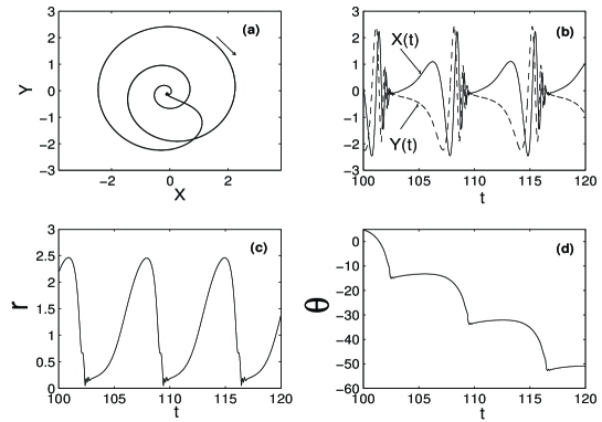
FIG. 15.: A spiraling orbit. The orbit of the limit cycle in the $X-Y$ space (a), the temporal evolution of the individual components $X$ and $Y$ (b), the amplitude $r$ (c), and that of the phase (d) as measured from the origin are plotted for $K_{2}=-3.,K_{1}=0.2,a=1,\omega=1$, and $\tau=0.5$.

5 Radially Trapped Solutions

As we cross the boundary of $FP_{1}$, the node $FP_{1}$ loses stability in a Hopf bifurcation as $K_{2}$ is increased resulting in a periodic orbit encircling $FP_{1}$. For negative $K_{2}$, the corresponding node is $FP_{2}$. These orbits have winding number zero around the origin and exist in the regions $BS_{1}$ and $BS_{2}$ bordering those marked $FP_{1}$ and $FP_{2}$. We call them radially trapped solutions because, viewed from the origin, they are restricted to a region of phase space and seem to oscillate within a restricted physical space. One such radially trapped orbit is shown in Fig. 14(a) with the corresponding bifurcation diagram in Fig. 14(b). The oscillator moves clockwise. Increased delay requires only weaker feedback to destabilize the node but the value saturates as shown in Fig. 14(c); the curve shown is plotted using Eq. (47) and is verified numerically.

6 Spiraling solutions and phase jumps

Another interesting periodic orbit that we find is shown in Fig. 15(a) and can best be described as a spiraling orbit since the amplitude of the limit cycle (in the $(X,Y)$ space) first spirals out and then comes back to its original state. The phase changes have a step like character and often exhibit large jumps. Such orbits exist in a thin region near the radially trapped solutions.

7 Birhythmicity

The phase reversing and the radially trapped solutions can also coexist in the same parameter regime (e.g. $K_{2}=-1.6$, $K_{1}=-0.2$, $a=1$, $\omega=1$, $\tau=0.5$ as shown in Fig. 16(a)) and thus exhibit a birhythmic behavior. In fact, birhythmicity appears to occur also for the spiraling and trapped solutions and is spread out over a large region of the parameter space inside $BS_{1}$ and $BS_{2}$ in Fig. 9. Birhythmicity is a common phenomenon in many biological cell models, and is currently the subject of many studies [42]. The switching between the two states can take place by the slightest perturbation to the initial states $(X(0),Y(0))$. A plot of the basins of attraction for the two states of Fig. 16(a) is shown in Fig. 16(b) in the space of the initial conditions $(X(0),Y(0))$. The dotted region is the basin of attraction for the phase reversing solution and the white region is that for the radially trapped solution. To generate this figure the initial conditions chosen were $X(\theta)=X(t=0),\theta\in[-\tau,0)$, and $Y(\theta)=Y(t=0),\theta\in[-\tau,0)$.

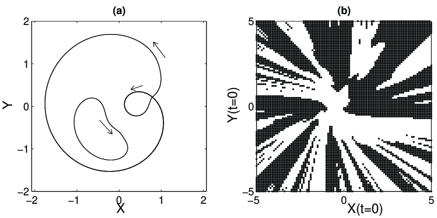
FIG. 16.: Birhythmicity between two periodic orbits. (a) Radially trapped and the phase reversal solution coexisting for $K_{2}=-1.6$, $K_{1}=-0.2$, $a=1$, $\omega=1$, and $\tau=0.5$. (b) A plot of the basins of attraction for these two states in the space of the initial conditions $(X(0),Y(0))$. The dotted region is the basin of attraction for the phase reversing solution and the white region is that for the radially trapped solution. To generate this figure the initial conditions chosen were $X(\theta)=X(t=0),\theta\in[-\tau,0)$, and $Y(\theta)=Y(t=0),\theta\in[-\tau,0)$.

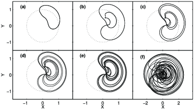
FIG. 17.: The radially trapped orbit of the limit cycle can undergo a period doubling sequence to the chaotic state. Some of the periodic orbits with (a) Period-1, $K_{2}=1.6$, (b) Period-2, $K_{2}=2.1$, (c) Period-4, $K_{2}=2.13$, (d) Period-8, $K_{2}=2.18$, (e) Period-16, $K_{2}=2.186$, and (f) a chaotic orbit, $K_{2}=2.6$ are shown. The other constants are $K_{1}=-0.2$, $a=1$, $\omega=1$, and $\tau=0.5$. The scale of (d) is twice that of the other plots.

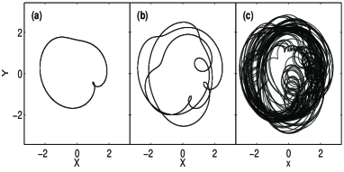
FIG. 18.: The phase reversing orbit can bifurcate into a period-3 orbit leading to a chaotic attractor. These typical states are shown for (a) $K_{2}=2.2$, (b) $K_{2}=2.5$, (c) $K_{2}=2.712$. The other constants are $K_{1}=4.2$, $a=1$, $\omega=1$, and $\tau=0.5$.

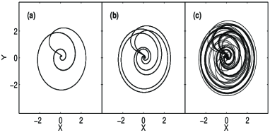
FIG. 19.: The spiraling orbit period doubles once and then goes to a chaotic state as typically shown in the sequence, (a) $K_{2}=3.0$, (b) $K_{2}=3.121$, (c) $K_{2}=3.128$. The other constants are $K_{1}=0.2$, $a=1$, $\omega=1$, and $\tau=0.5$.

FIG. 20.: Typical bifurcation diagrams generated by Poincare section techniques showing (a) phase trapped, (b) phase reversing, and (c) spiraling solutions. The plots show the value of (a) $X$ in the plane $Y=0$, $\dot{Y}<0$, $K_{1}=-0.25$, (b) $Y$ in the plane $X=-1.4$, $\dot{X}<0$, $K_{1}=4.3$ and (c) $X$ in the plane $Y=-2.$, $\dot{Y}<0$, $K_{1}=0.2$. The other constants are $a=1,~{}\omega=1,$ and $\tau=0.5$.

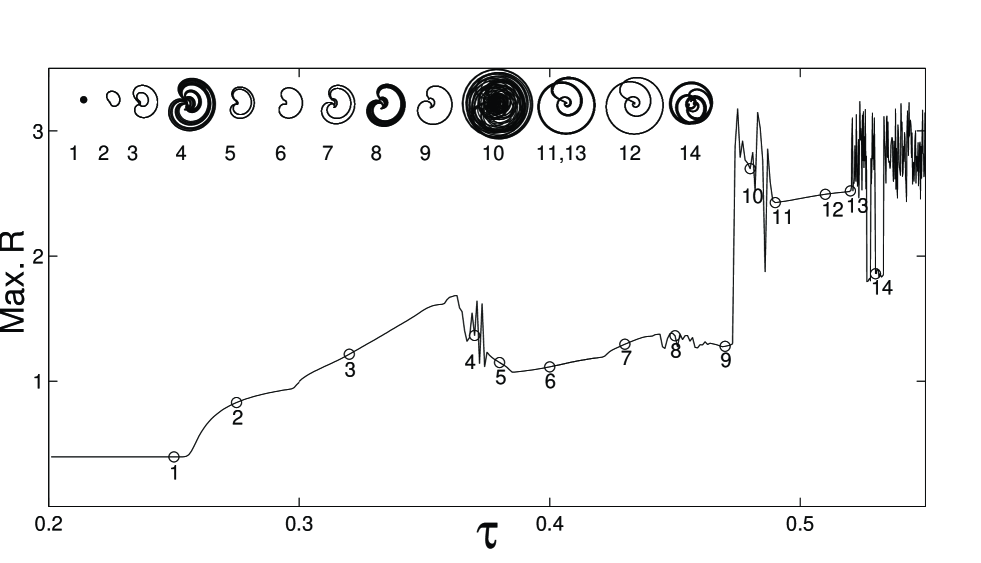
FIG. 21.: Bifurcation diagram as a function of $\tau$. $R$ is the maximum value of the amplitude of the oscillator as a function of $\tau$ for $K_{2}=-3.0$, and $K_{1}=0.2,a=1$, and $\omega=1$. The initial conditions used are $X(0)=0.123$, $Y(0)=0.456$. The orbits at various points that are numbered are shown in the inset. The orbit at $11$ and $13$ is the spiraling orbit with period-2.

8 Routes to Chaos

The nonlinear model equation (34) also exhibits regions of temporal chaos and we have investigated this phenomenon in some detail, particularly with regard to routes to chaos. The route to chaos appears to be a strong function of the parameters $K_{1},K_{2}$ and $\tau$ and the type of periodic orbit existing in a particular parameter domain. There is evidence of several distinct routes to chaos in the present model system. For example, the radially trapped solutions appear to follow the period doubling route to chaos as shown in the sequence of plots in Fig. 17. The phase reversing solutions appear to go to the chaotic state in several different ways. The limit cycle can make a transition from a simple orbit to a quasi-periodic state. It can also period double. Or a period 1 state can make a transition to a period-3 orbit. Such a transition is shown in Fig. 18. We find a large window of Period-3 orbits starting from $K_{2}=2.283$ for the parameters given in Fig. 18. The spiraling orbits appear to undergo a single period doubling bifurcation and then a sudden transition to chaos. An example is shown in Fig. 19. Finally, in Fig. 20, we display the detailed bifurcation diagrams (obtained from Poincare section plots) corresponding to these scenarios. We would like to add a word here about the numerical precautions followed in generating these diagrams. Since many of these attractors can coexist in a birhythmic state, it is necessary to adopt high accuracy and care in tracking any one of them. Likewise one also needs to get beyond some long transients that the system can exhibit for some particular initial conditions. Using these precautions, in Fig. 21, we have given a detailed bifurcation diagram as a function of the time delay parameter. In this, the maximum amplitude of the oscillator is plotted for $K_{1}=0.2,K_{2}=-3.0$ at various values of $\tau$. The various numbers on the curves stand for the kind of orbit that is found in that region (a phase portrait of the orbit is also depicted for reference). The initial conditions chosen have been $X(0)=0.123$ and $Y(0)=0.456$.

IV Summary and Discussion

We have studied the dynamics of a single Hopf bifurcation oscillator (the Stuart-Landau equation) in the presence of an autonomous time delayed feedback. The feedback term has both a linear component and a simple quadratic nonlinear term. Using a combination of analytical methods and numerical analysis, we have investigated the temporal dynamics of this system in various regimes characterized by the natural parameters of the oscillator (e.g. its frequency $\omega$, linear growth rate $a$), strengths of the feedback components ($K_{1}$, $K_{2}$) and the time delay parameter, $\tau$. Our principle results are presented in the form of bifurcation diagrams in these parameter spaces. These reveal a rich variety of temporal behavior including time delay induced stabilization of the origin, multiple frequency states, frequency suppression, phase slips, saddle node bifurcations, and chaotic behavior. In addition, some of the periodic orbits exhibit novel behavior such as birhythmicity, phase reversals, radial trapping, spiraling oscillations in amplitude space. Some of these can be understood by the stability of the fixed points or the loss of single valuedness of amplitude evolution equation.

One of the attractive features of these results is that many of them have been observed in the collective behavior of larger systems such as the Kuramoto model or the amplitude versions of the Kuramoto model. This has been one of our major motivations for constructing this model - as a sort of paradigm to obtain and investigate these states in a simple manner. The feedback terms not only model the collective drive that a single oscillator feels in a larger system, but also incorporate time delay in an autonomous manner. Time delay frees the dimensional constraints of the system (the system is essentially $\infty$ -dimensional) and this might be the reason why its temporal dynamics resembles so much that of larger dimensional systems. Our results may therefore be useful for gaining better insights into the behavior of such large systems. As an example, the large window of $W-3$ orbits of our model appears to have a correspondence to the transition region between the incoherent and chaotic states of coupled limit cycle oscillators. We have found that the oscillators in the wings of the frequency distribution of a large collection of oscillators in the mean field model begin to acquire the $W-3$ temporal states in that region and play an important role in the transition mechanism [47]. A detailed understanding of their dynamical behavior can thus help us in addressing some of the outstanding problems in this area, such as the nature of transition between low dimensional chaos and turbulence. Our model can also find more direct applications in simulation studies for feedback control of individual physical, chemical or biological entities that have the basic nonlinear characteristics of our Hopf oscillator, such as in single mode semiconductor lasers, relativistic magnetrons, chemical oscillations, and biological rhythms in single nerve cells. In fact, the basic Stuart-Landau equation is mathematically related to the well known van der Pol oscillator equation from which it can be derived by a suitable time averaging. Our oscillator model with the quadratic nonlinearity can likewise be derived from a van der Pol type equation which in addition has a nonlinear Mathieu like term, i.e., it is an equation of the form

$$\ddot{x}+\mu~{}(x^{2}-1)\dot{x}+(1+~{}\epsilon~{}\dot{x}~{}\sin(t))~{}x=0.$$ (52)

Such a nonlinear equation can physically represent parametric excitation of relaxation oscillations and can be used to model a number of physical or biological systems. It may be possible in such simple systems to then seek experimental verification of some of the novel temporal states displayed by our model.

REFERENCES

- [1] E-mail: tapovan@plasma.ernet.in
- [2] E-mail: abhijit@plasma.ernet.in
- [3] M. K. McClintock, Menstrual Synchrony and Suppression, Nature 229 (1971) 244.
- [4] P. DeNeef, H. Lashinsky, Van der Pol model for unstable waves on a beam-plasma system, Phys. Rev. Lett. 31 (1973) 1039.
- [5] A. T. Winfree, The Geometry of Biological Time, Springer-Verlag, New York, 1980.
- [6] A. T. Winfree, The Three-Dimensional Dynamics of Electrochemical Waves and Cardiac Arrhythmias, Princeton University Press, Princeton, NJ, 1987.
- [7] Y. Kuramoto, I. Nishikawa, Statistical macrodynamics of large dynamical systems. Case of a phase transition in oscillator communities, J. Stat. Phys. 49 (1987) 569.
- [8] J. Benford, H. Sze, W. Woo, R. R. Smith, B. Harteneck, Phase Locking of Relativistic Magnetrons, Phys. Rev. Lett. 62 (1989) 969.
- [9] D. Golomb, D. Hansel, B. Shraiman, H. Sompolinsky, Clustering in globally coupled phase oscillators, Phys. Rev. A 45 (1992) 3516.
- [10] S. I. Doumbouya, A. F. Munster, C. J. Doona, F. W. Schneider, Deterministic chaos in serially coupled chemical oscillators, J. Phys. Chem. 97 (1993) 1025.
- [11] J. J. Collins, I. N. Stewart, Coupled Nonlinear Oscillators and the Symmetries of Animal Gaits, J. Nonlinear Sci. 3 (1993) 349.
- [12] H. Daido, Onset of cooperative entrainment in limit-cycle oscillators with uniform all-to-all interactions: bifurcation of the order function, Physica D 91 (1996) 24, and references therein.
- [13] L. M. Pecora, Synchronization conditions and desynchronizing patterns in coupled limit-cycle and chaotic systems, Phys. Rev. E 58 (1998) 347.
- [14] K. Nakajima, Y. Sawada, Experimental studies on the weak coupling of oscillatory chemical reaction systems, J. Chem. Phys. 72 (1980) 2231.
- [15] K. Bar-Eli, On the stability of coupled chemical oscillators, Physica D 14 (1985) 242.
- [16] D. G. Aronson, G. B. Ermentrout, N. Koppel, Amplitude response of coupled oscillators, Physica D 41 (1990) 403.
- [17] P. C. Matthews, S. H. Strogatz, Phase diagram for the collective behavior of limit cycle oscillators, Phys. Rev. Lett. 65 (1990) 1701.
- [18] P. C. Matthews, R. E. Mirollo, S. H. Strogatz, Dynamics of a large system of coupled nonlinear oscillators, Physica D 52 (1991) 293, and references therein.
- [19] H. G. Schuster, P. Wagner, Mutual entrainment of two limit cycle oscillators with time delayed coupling, Prog. Theor. Phys. 81 (1989) 939.
- [20] E. Niebur, H. G. Schuster, D. Kammen, Collective frequencies and metastability in networks of limit-cycle oscillators with time delay, Phys. Rev. Lett. 67 (1991) 2753.
- [21] Y. Nakamura, F. Tominaga, T. Munakata, Clustering behavior of time-delayed nearest-neighbor coupled oscillators, Phys. Rev. E 49 (1994) 4849.
- [22] S. Kim, S. H. Park, C. S. Ryu, Multistability in coupled oscillator systems with time delay, Phys. Rev. Lett. 79 (1997) 2911.
- [23] D. V. R. Reddy, A. Sen, G. L. Johnston, Time delay induced death in coupled limit cycle oscillators, Phys. Rev. Lett 80 (1998) 5109.
- [24] D. V. R. Reddy, A. Sen, G. L. Johnston, Time delay effects on coupled limit cycle oscillators at Hopf bifurcation, Physica D 129 (1999) 15.
- [25] M. K. S. Yeung, S. H. Strogatz, Time delay in the Kuramoto model of coupled oscillators, Phys. Rev. Lett. 82 (1999) 648.
- [26] P.C. Bressloff, S. Coombes, Travelling Waves in chains of pulse-coupled integrate-and-fire oscillators with distributed delays, Physica D 130 (1999) 232.
- [27] A. Callender, D. R. Hartree, A. Porter, Time-Lag in a Control System, Phil. Trans. Roy. Soc. London A 235 (1936) 415.
- [28] W. K. Ergen, Kinetics of the Circulating-Fuel Nuclear Reactor, J. Appl. Phys. 25 (1954) 702.
- [29] R. D. Driver, A Two-Body Problem of Classical Electrodynamics: the One-Dimensional Case, Ann. Phys. 21 (1963) 122.
- [30] W. Wischert, A. Wunderlin, A. Pelster, M. Olivier, J. Groslambert, Delay-induced instabilities in nonlinear feedback systems, Phys. Rev. E 49 (1994) 203.
- [31] K. Miyakawa, K. Yamada, Entrainment in coupled salt-water oscillators, Physica D 127 (1999) 177.
- [32] P. Tass, J. Kurths, M. G. Rosenblum, G. Guasti, H. Hefter, Delay-induced transitions in visually guided movements, Phys. Rev. E 54 (1996) R2224.
- [33] A. Destexhe, Stability of periodic oscillations in a network of neurons with time delay, Phys. Lett. A 187 (1994) 309.
- [34] J. M. Cushing, Periodic Solutions of Volterra’s Population Equation with Hereditary Effects, SIAM J. Appl. Math. 31 (1976) 251.
- [35] S. A. Campbell, J. Bélair, T. Ohira, J. Milton, Complex dynamics and multistability in a damped harmonic oscillator with delayed negative feedback, Chaos 5 (1995) 640.
- [36] A. Fraikin, H. Lemarchand, Stochastic analysis of a Hopf bifurcation: Master equation approach, J. Stat. Phys. 41 (1985) 531.
- [37] M. C. Mackey, A.Longtin, A. Lasota, Noise-induced global asymptotic stability, J. Stat. Phys. 60 (1990) 735.
- [38] C. Kurrer, K. Schulten, Effect of noise and perturbations on limit cycle systems, Physica D 50 (1991) 311.
- [39] K. Pyragas, Continuous control of chaos by self-controlling feedback, Phys. Lett. A 170 (1992) 421.
- [40] O. Diekmann, S. A. van Gils, S. M. Verduyn Lunel, H.-O. Walther, Delay Equations: Functional-, Complex-, and Nonlinear Analysis, Springer-Verlag, New York, 1995, Ch. XI.
- [41] R. D. Driver, Ordinary and Delay Differential Equations, Springer-Verlag, New York, 1977.
- [42] A. Goldbeter, Biological Oscillations and Cellular Rhythms, Cambridge University Press, Cambridge, 1996.
- [43] Z. Zheng, G. Hu, B. Hu, Phase Slips and Phase Synchronization of Coupled Oscillators, Phys. Rev. Lett. 81 (1998) 5318.
- [44] C. T. H. Baker, C. A. H. Paul, D. R. Willé, Issues in the Numerical Solution of Evolutionary Delay Differential Equations, Numerical Analysis Report No. 248, Department of Mathematics, University of Manchester, Manchester M13 9PL, England, and references therein.
- [45] S. Sato, M. Sano, Y. Sawada, Universal Scaling Property in Bifurcation Structure of Duffing’s and of generalized Duffing’s Equation, Phys. Rev. A 28 (1983) 1654.
- [46] J. Guckenheimer, P. J. Holmes, Nonlinear Oscillations, Dynamical Systems, and Bifurcations of Vector Fields, Springer-Verlag, New York, 1983.
- [47] D. V. R. Reddy, A. Sen, G. L. Johnston, (to be published).