The multifractal structure of chaotically advected chemical fields

Abstract

The structure of the concentration field of a decaying substance produced by chemical sources and advected by a smooth incompressible two-dimensional flow is investigated. We focus our attention on the non-uniformities of the Hölder exponent of the resulting filamental chemical field. They appear most evidently in the case of open flows where irregularities of the field exhibit strong spatial intermittency as they are restricted to a fractal manifold. Non-uniformities of the Hölder exponent of the chemical field in closed flows appears as a consequence of the non-uniform stretching of the fluid elements. We study how this affects the scaling exponents of the structure functions, displaying anomalous scaling, and relate the scaling exponents to the distribution of finite-time Lyapunov exponents of the advection dynamics. Theoretical predictions are compared with numerical experiments.

I Introduction

Mixing in fluids plays an important role in nature and technology with implications in areas ranging from geophysics to chemical engineering[1]. The phenomenon of chaotic advection – intensively investigated during the last decade – provides a basic mechanism for mixing in laminar flows[2]. Briefly stated, chaotic advection refers to the situation in which fluid elements in a non-turbulent flow follow chaotic trajectories. Advection by simple time-dependent two-dimensional flows falls generically under this category. Stirring by chaotic motion, with its characteristic stretching and folding of material elements, is able to bring distant parts of the fluid into intimate contact and thus greatly enhances mixing by molecular diffusion acting at small scales.

Mixing efficiency becomes specially important when the substances advected by the flow are not inert but have some kind of activity. By ‘activity’ we mean that some time-evolution is occurring to the concentrations inside advected fluid elements (produced by chemical reactions, for example). For definiteness we will use terms such as chemical fields and chemical reactions, but biological processes, occurring for example when the advected substance is living plankton, can be described formally in the same way. The interaction between the stirring process and the chemical activity can result in complex patterns for the spatial distribution of the chemical fields, which in turn greatly affect the chemical processes[3, 4]. In addition to the impact on its own chemical dynamics, the spatial inhomogeneities may have important effect on other dynamical processes occurring in the fluid (for example in the behavior of predators seeking for the advected plankton [5]). An understanding of the structure of these spatial patterns is thus valuable.

Previous theoretical work concentrated on the temporal evolution of the total amount of chemical products in specific reactions such as $A+B\rightarrow 2C$ or $A+B\to 2B$ [6]. In [7] the same type of reactions were studied in open flows. In a previous paper [8] some of us considered a class of chemical dynamics characterized by a negative Lyapunov exponent in the presence of (non-homogeneous) chemical sources. Under such chemical processes, reactant concentrations present a tendency to relax towards a local-equilibrium concentration (the fixed point of the local chemical dynamics). This tendency is disrupted by the advection process, which forces fluid elements to visit places with different local-equilibrium states. Depending on the relative strength of chaotic advection and relaxation the resulting concentration distribution can be smooth (differentiable) or exhibits characteristic filamental patterns that are nowhere differentiable except in the direction of filaments aligned with the unstable foliation induced in the fluid by the chaotic dynamics. The mechanism for the appearance of these singular filaments is similar to the one producing singular invariant measures in dynamical systems [9], although here it is affected by the presence of the chemical dynamics: stretching by the flow homogeneizes the pattern along unstable directions, whereas small-scale variance, cascading down from larger scales, accumulates along the stable directions, producing diverging gradients.

The strength of the singularities of the concentration field $C({\bf r})$ can be characterized by a Hölder exponent $\alpha$

$$|\delta C({\bf r_{0}};{\bf\delta r})|\equiv|C({\bf r_{0}}+{\bf\delta r})-C({\bf r_{0}})|\sim|{\bf\delta r}|^{\alpha},\;\;\;|{\bf\delta r}|\rightarrow 0\ .$$ (1)

If the field is smooth (differentiable) at $\bf r_{0}$, $\alpha=1$, while for an irregular rough (e.g. filamental) structure $0<\alpha<1$. In [8] we focused on the existence of a smooth-filamental transition as time-scales of the system are varied, and also obtained the most probable (bulk) value of the Hölder exponent. Note, however, that the Hölder exponent defined by (1) is a local characteristic of the field, whose value may depend on the position ${\bf r_{0}}$. In this Paper we concentrate on such non-uniformities of the filamental chemical field and study how this affects scaling properties of quantities involving spatial averages, which are the more convenient quantities to be observed in experiments.

In Section II we review the results presented in [8], namely the smooth-filamental transition and the dominant value of the Hölder exponent in closed flows. Then we consider the same problem for the case of mixing by open flows (Sect. III). In this case the necessity of a multifractal description becomes manifest, and this motivates the development of a quantitative characterization of the filamental structures in terms of structure functions. This is presented in Sect. IV. Scaling exponents appear to be related to the distribution of finite-time Lyapunov exponents. We conclude the Paper with a summary and discussion.

II The smooth-filamental transition

We consider the flow as externally prescribed, thus neglecting any back influence of the chemical dynamics into the hydrodynamics (the advected substances are chemically active but hydrodynamically passive). In this context, the general continuum description of chemical reactions in hydrodynamic flows is given by sets of reaction-advection-diffusion equations. They involve in general multiple components and nonlinear reaction terms. Reference [8] considered the situation in which the chemical kinetics is stable, i.e. there is a local-equilibrium state at each spatial position, determined by the sources and the reaction terms, so that concentrations of fluid particles visiting that position tend to relax to the local-equilibrium value. Mathematically this corresponds to the negativity of the Lyapunov exponents associated to the chemical dynamical subsystem. It was shown in [8] that arbitrary chemical dynamics in this class can be substituted by linear relaxation towards local equilibrium at a rate given by the largest (least negative) chemical Lyapunov exponent. Within this restriction, the multiplicity of components is not essential since, except for special types of coupling, linearization leads to simple relations between the different fields.

Because of the above remarks, and with the aim of keeping the mathematics as simple as possible, we will restrict our considerations in this Paper to the simplest chemical evolution: linear decay, at a rate $b$, of a single advected substance. A space-dependent source of the substance will also be included, to maintain a non-trivial concentration field at long times. This chemical dynamics can be considered either as an approximation to more complex chemical or biological evolutions, with maximum chemical Lyapunov exponent $-b$, or as a description of simple specific processes such as spontaneous decomposition of unstable radicals, decay of a radioactive substance, or relaxation of sea-surface temperature towards atmospheric values [10]. The validity of our ideas for nonlinear multicomponent situations has been checked for a plankton model in [11].

The concentration field $C({\bf r},t)$, when advected by a incompressible velocity field ${\bf v}({\bf r},t)$ is governed by the equation

$$\frac{\partial C}{\partial t}+{\bf v}({\bf r},t)\cdot\nabla C=S({\bf r})-bC+\kappa\nabla^{2}C,$$ (2)

where $\kappa$ is the diffusion coefficient, $b$ is the decay rate introduced above and $S({\bf r})$ is the concentration input from chemical sources (negative values representing sinks). We restrict our study to the case in which the incompressible velocity field is two-dimensional, smooth, and non-turbulent. Chaotic advection is obtained generically if a simple time-dependence, for example periodic, is included in ${\bf v}({\bf r},t)$. We assume that diffusion is weak and transport is dominated by advection. Thus one expects that the distribution on scales larger than a certain diffusive scale is not affected by diffusion. Therefore we consider the limiting non-diffusive case $\kappa=0$. In this limit the above problem can be described in a Lagrangian picture by an ensemble of ordinary differential equations

$$\frac{d{\bf\hat{r}}}{dt}={\bf v}({\bf\hat{r}},t),$$ (3)

$$\frac{d\hat{C}}{dt}=S[{\bf\hat{r}}(t)]-b\hat{C},\;$$ (4)

where the solution of the first equation gives the trajectory of a fluid parcel, ${\bf\hat{r}}(t)$, while the second one describes the Lagrangian chemical dynamics in this fluid element: $\hat{C}(t)\equiv C[{\bf r}={\bf\hat{r}}(t),t]$.

To obtain the value of the chemical field at a selected point ${\bf\bar{r}}$ at time $\bar{t}$ one needs to know the previous history of this fluid element, that is the trajectory ${\bf\hat{r}}(t)$ ($0\leq t\leq\bar{t}$) with the property ${\bf\hat{r}}(\bar{t})={\bf\bar{r}}$. This can be obtained by the integration of (3) backwards in time. Once ${\bf\hat{r}}(t)$ has been obtained, the solution of (4) is

$$C({\bf\bar{r}},\bar{t})=C[{\bf\hat{r}}(0),0]e^{-b\bar{t}}+\int_{0}^{\bar{t}}S[{\bf\hat{r}}(t)]e^{-b(\bar{t}-t)}dt.$$ (5)

One can obtain the difference at time $\bar{t}$ of the values of the chemical field at two different points ${\bf\bar{r}}$ and ${\bf\bar{r}}+\bar{\delta{\bf r}}$ separated by a small distance $\bar{\delta{\bf r}}$ in terms of the difference $C[{\bf\hat{r}}(t)+\hat{\delta{\bf r}}(t),t]-C[{\bf\hat{r}}(t),t]\equiv\delta C[{\bf\hat{r}}(t),t;\hat{\delta{\bf r}}(t)]$ for $0\leq t\leq\bar{t}$, namely:

$$\delta C({\bf\bar{r}},\bar{t};\bar{\delta{\bf r}})=\delta C[{\bf\hat{r}}(0),0;\hat{\delta{\bf r}}(0)]e^{-b\bar{t}}$$ (6)

$$+\int_{0}^{\bar{t}}\delta S[{\bf\hat{r}}(t);\hat{\delta{\bf r}}(t)]e^{-b(\bar{t}-t)}dt$$ (7)

where ${\hat{\delta{\bf r}}}(t)$ ($0\leq t\leq\bar{t}$) is the time-dependent distance between the two trajectories that end at ${\bf\bar{r}}$ and ${\bf\bar{r}}+\bar{\delta{\bf r}}$ at time $\bar{t}$, and $\delta S$, in analogy with $\delta C$, is the difference of the source term at points ${\bf\hat{r}}(t)$ and ${\bf\hat{r}}(t)+\hat{\delta{\bf r}}(t)$.

Thus we have expressed the behavior of an Eulerian quantity $\delta C({\bf\bar{r}},\bar{t};\bar{\delta{\bf r}})$ in terms of Lagrangian quantities, in particular of $\hat{\delta{\bf r}}(t)$. Further analysis of Eq. (7) requires specification of the behavior of $\hat{\delta{\bf r}}$. The signature of chaotic advection is the exponentially growing behavior of this quantity at long times. More precise statements need additional assumptions on the character of the flow. The simplest framework is obtained if we restrict our attention to initial conditions ${\bf\hat{r}}(0)$ in an invariant hyperbolic set [9]. In this case one can identify at each point two directions, the one in which the flow is contracting ${\bf c}({\bf r})$ and the expanding direction ${\bf e}({\bf r})$. They depend continuously on position (for time-dependent flows there is an additional explicit time-dependence that we do not write down to simplify the notation). Since ${\bf c}$ and ${\bf e}$ form at each point a vector basis which is not orthonormal, it is convenient to introduce also the dual basis (${\bf c^{\dagger}},{\bf e^{\dagger}}$) at each point. Chaotic advection manifests in which for most initial separations $\hat{\delta{\bf r}}(0)$ the long-time behavior of $\hat{\delta{\bf r}}$ is $|\hat{\delta{\bf r}}(t)|\sim\left|{\bf e}[{\bf\hat{r}}(0)]^{\dagger}\cdot\hat{\delta{\bf r}}(0)\right|e^{\lambda t}$ (for $t>0$), where $\lambda$ is the positive Lyapunov exponent of the flow and ${\bf e}[{\bf\hat{r}}(0)]^{\dagger}\cdot\hat{\delta{\bf r}}(0)$ gives the component of the initial separation along the expanding direction. At long times, the direction of $\hat{\delta{\bf r}}(t)$ tends to become aligned with the expanding direction of the flow at ${\bf\hat{r}}(t)$, ${\bf e}[{\bf\hat{r}}(t)]$. However, if the initial separation is aligned with the contracting direction at the initial point, $\lambda$ should be substituted by $\lambda^{\prime}$, the contractive Lyapunov exponent, and ${\bf e}^{\dagger}$ by ${\bf c}^{\dagger}$. For incompressible flows one has $\lambda^{\prime}=-\lambda$.

In order to analyze (7) one has to consider the backwards evolution. In this case typical solutions behave, for $t<0$ and large, as $|\hat{\delta{\bf r}}(t)|\sim\left|{\bf c}[{\bf\hat{r}}(0)]^{\dagger}\cdot\hat{\delta{\bf r}}(0)\right|e^{\lambda^{\prime}t}=\left|{\bf c}[{\bf\hat{r}}(0)]^{\dagger}\cdot\hat{\delta{\bf r}}(0)\right|e^{-\lambda t}$ so that, also in this backwards dynamics, close initial conditions diverge, and the difference will tend to become aligned with the most expanding direction of the backwards flow (the contracting of the forward flow, ${\bf c}[{\bf\hat{r}}(t)]$). Again, there is a particular direction for the orientation of the initial condition (the contracting one in the backwards flow which is the expanding one in the forward dynamics) for which $-\lambda$ should be replaced by $\lambda$. In (7), $\hat{\delta{\bf r}}$ is obtained backwards starting from $\bar{\delta{\bf r}}$ at $t=\bar{t}$. In this case:

$$\hat{\delta{\bf r}}(t)\approx{\bf c({\bf\bar{r}})}^{\dagger}\cdot\bar{\delta{\bf r}}\ e^{\lambda(\bar{t}-t)}{\bf c}[{\bf\hat{r}}(t)]\ ,\;\;t_{s}\leq t\leq\bar{t}\ .$$ (8)

The exponential separation (8) holds only while the distance $\hat{\delta{\bf r}}(t)$ is not too large, and saturates when approaching the size of the system or some characteristic coherence length of the velocity field. The time at which this happens defines $t_{s}$, a saturation time. We assume that both the velocity field and the source $S({\bf r})$ have only large-scale structures such that their corresponding coherence lengths are comparable to the system size, that we take as the unit of length-scales. Thus, the saturation time is given by $t_{s}=\bar{t}+\lambda^{-1}\ln|\bar{\delta{\bf r}}|$.

For small $\bar{\delta{\bf r}}$, Eq. (7) can be written as

$$\delta C({\bf\bar{r}},\bar{t};\bar{\delta{\bf r}})\approx\delta C[{\bf\hat{r}}(0),0;\hat{\delta{\bf r}}(0)]e^{-b\bar{t}}$$ (9)

$$+\int_{0}^{t_{s}}\delta S[{\bf\hat{r}}(t);\hat{\delta{\bf r}}(t)]e^{-b(\bar{t}-t)}dt$$ (10)

$$+\int_{t_{s}}^{\bar{t}}\hat{\delta{\bf r}}(t)\cdot\nabla S[{\bf\hat{r}}(t)]e^{-b(\bar{t}-t)}dt$$ (11)

(if $t_{s}>0$). We will not need to specify the dependence of $\delta S$ on $\hat{\delta{\bf r}}$ for times previous to $t_{s}$, as long as $\delta S$ remains bounded. Substitution of (8) in the second integral leads to

$$\delta C({\bf\bar{r}},\bar{t};\bar{\delta{\bf r}})\approx\delta C[{\bf\hat{r}}(0),0;\hat{\delta{\bf r}}(0)]e^{-b\bar{t}}$$ (12)

$$+\int_{0}^{t_{s}}\delta S[{\bf\hat{r}}(t);\hat{\delta{\bf r}}(t)]e^{-b(\bar{t}-t)}dt$$ (13)

$$+\bar{\delta{\bf r}}\cdot{\bf c({\bf\bar{r}})}^{\dagger}\int_{t_{s}}^{\bar{t}}{\bf c}[{\bf\hat{r}}(t)]\cdot\nabla S[{\bf\hat{r}}(t)]e^{(\lambda-b)(\bar{t}-t)}dt$$ (14)

Taking the limit $\bar{\bf\delta r}\rightarrow 0$ (for a finite $\bar{t}$) leads to $t_{s}<0$. Thus the first integral disappears and the first term can be linearized. By writing $\bar{\delta{\bf r}}=\bar{\bf n}|\bar{\delta{\bf r}}|$ so that $\bar{\bf n}$ is a unit vector, one finds the directional derivative along the direction of $\bar{\bf n}$ as

$$\bar{\bf n}\cdot\nabla C({\bf\bar{r}},\bar{t})\approx\bar{\bf n}\cdot{\bf c({\bf\bar{r}})}^{\dagger}{\bf c}[{\bf\hat{r}}(0)]\cdot\nabla C[{\bf\hat{r}}(0),0]e^{(\lambda-b)\bar{t}}$$ (15)

$$+\bar{\bf n}\cdot{\bf c({\bf\bar{r}})}^{\dagger}\int_{0}^{\bar{t}}{\bf c}[{\bf\hat{r}}(t)]\cdot\nabla S[{\bf\hat{r}}(t)]e^{(\lambda-b)(\bar{t}-t)}dt\ .$$ (16)

If $\lambda<b$ this derivative remains finite in the $\bar{t}\rightarrow\infty$ limit and the asymptotic field $C_{\infty}({\bf\bar{r}})\equiv C({\bf r},\bar{t}\rightarrow\infty)$ is smooth (differentiable). Otherwise the derivatives of $C$ diverge as $\sim e^{(\lambda-b)\bar{t}}$ leading to a nowhere-differentiable irregular asymptotic field. The exception again is the expanding direction of the forward flow: when $\bar{\delta{\bf r}}$ points along that direction one should substitute in Eq. (16) $\lambda$ and ${\bf c}$ by $-\lambda$ and ${\bf e}$. This directional derivative is always finite. Thus, there is at each point a direction along which $C_{\infty}$ is smooth. By changing the values of $b$ and $\lambda$ one will encounter, at $b=\lambda$ a morphological transition between a smooth pattern and a filamental (i.e., singular in all but one directions) one. It should be noted that, because the explicit time-dependence of the vectors ${\bf c}$ and ${\bf e}$ referred to before, the limiting distribution $C_{\infty}$ will not be a steady field, but one following the time dependence of the stable and unstable directions. For time-periodic flows ${\bf v}({\bf r},t)$, $C_{\infty}$ will also be time periodic. Its singular characteristics however do not change in time.

In order to characterize the singular asymptotic field we take the limit $\bar{t}\rightarrow\infty$ for fixed finite $\bar{\bf\delta r}$ in (14)

$$\delta C_{\infty}({\bf\bar{r}};\bar{\delta{\bf r}})\approx\int_{|\bar{\delta{\bf r}}|^{-1/\lambda}}^{\infty}\delta S[{\bf\hat{r}}(x);\hat{\delta{\bf r}}(x)]x^{-b-1}dx$$ (17)

$$+|\bar{\delta{\bf r}}|\bar{\bf n}\cdot{\bf c({\bf\bar{r}})}^{\dagger}\int_{1}^{|\bar{\delta{\bf r}}|^{-1/\lambda}}{\bf c}[{\bf\hat{r}}(x)]\cdot\nabla S[{\bf\hat{r}}(x)]x^{\lambda-b-1}dx$$ (18)

where we used the change of variables $e^{\bar{t}-t}\rightarrow x$. If $b>\lambda$ one finds for the dominant term in the $|\bar{\bf\delta r}|\rightarrow 0$ limit the simple scaling $\delta C_{\infty}\sim|\bar{\delta{\bf r}}|$, but when $b<\lambda$:

$$\delta C_{\infty}({\bf\bar{r}};\bar{\delta{\bf r}})\sim|\bar{\delta{\bf r}}|^{\frac{b}{\lambda}}\ .$$ (19)

According to (1) the value of the Hölder exponent is

$$\alpha=\min\left\{\frac{b}{\lambda},1\right\}.$$ (20)

This implies that if $b<\lambda$ the asymptotic chemical field becomes an irregular fractal object (again there is an orientation of $\bar{\delta{\bf r}}$ along which $\alpha=1$). Consequently, the graph of the field along a one-dimensional cut or transect, or the contours of constant concentration are also fractals, as they are two-dimensional sections of the whole $C_{\infty}(\bf r)$ embedded in a three-dimensional space. More precisely, the one-dimensional transect (along the direction $x$) of the field is a self-affine function with its graph embedded in an inherently anisotropic space ($C-x$) with axis representing different physical quantities. Contours of constant concentrations, however, are self-similar fractal sets of the two-dimensional physical space ($x-y$).

In Figs. 1 and 2 we present snapshots of the asymptotic field $C_{\infty}$ evolving according to (3)-(4). For the flow we take a simple time-periodic velocity field defined in the unit square with periodic boundary conditions by

$$v_{x}(x,y,t) = -\frac{2U}{T}\Theta\Bigl{(}\frac{T}{2}-t\bmod T\Bigr{)}\cos({2\pi y})$$ (21)

$$v_{y}(x,y,t) = -\frac{2U}{T}\Theta\Bigl{(}t\bmod T-\frac{T}{2}\Bigr{)}\cos({2\pi x})$$ (22)

where $\Theta(x)$ is the Heavyside step function. In our simulations $U=1.2$, which produces a flow with a single connected chaotic region. The value of the numerically obtained Lyapunov exponent is $\lambda\approx 2.67/T$.

Backward trajectories with initial coordinates on a rectangular grid were calculated and used to obtain the chemical field at each point by using (5) forward in time with the source term $S(x,y)=1+\sin{(2\pi x)}\sin{(2\pi y)}$. The values of the parameters used in Fig. 1 are $T=1.0$ and $b=4.0$, for which the Lyapunov exponent is $\lambda=2.67<b$. A smooth pattern is seen, in agreement with our theoretical arguments. In Fig. 2 the parameters are $T=1.0$ and $b=0.1$, so that $\lambda>b$ and a filamental pattern is obtained.

The smooth-fractal transition also appears in the time-dependence of the concentration measured at a fixed point in space. This can be shown by a similar analysis for the difference

$$\delta C({\bf r},t;\delta t)\equiv C({\bf r},t+\delta t)-C({\bf r},t)$$ (23)

instead of the spatial difference discussed above. If $b<\lambda$ the signal $C({\bf r},t)$ becomes non-differentiable in time and can be characterized by the same Hölder exponent $b/\lambda$. The fact that scaling properties of the temporal signal and that of the spatial structure are the same –analogously to the so called ‘Taylor hypothesis’ in turbulence– can be exploited in experiments or in analysis of geophysical data.

We conclude with some comments on the range of validity of Eq. (16). The Lagrangian description (3)-(4) in which our approach is based is valid only for scales at which diffusion is negligible. Thus there is a minimum admissible value $l_{diff}(\kappa)\sim\sqrt{\kappa}$ of $\bar{\delta{\bf r}}$ and our calculation should be understood as giving the gradients only up to this scale, fractality being washed out at smaller scales by the presence of diffusion. Nevertheless we think that, if diffusion is weak, the fractal-filamental transition will be seen at scales larger than this diffusive scale. For fixed $\bar{\delta{\bf r}}$ larger than the diffusion length, (14) remains valid until a time $\bar{t}\lesssim t_{s}(\bar{\delta{\bf r}})$ that means that the divergence of the gradients will also saturate at a finite value $\sim(l_{diff})^{b/\lambda-1}$.

Another limitation to the validity of our equations arises from the fact that, for most chaotic flows of physical relevance, not all the points visited by the fluid particle will be hyperbolic. The stable and unstable directions in the previous discussion become tangent at some points and equations such as (14) become undefined there. More importantly, KAM tori will be present in the system, so that for values of ${\bf\bar{r}}$ lying on KAM trajectories the value of the Lyapunov exponent appearing in (8) will not be positive but zero. These facts imply that our previous equations are not valid in a global sense. The main effect of the KAM tori will be to partition space into ergodic regions. Each region will be characterized by a different value of $\lambda$, and there is the possibility of observing different morphologies in the different regions. For the values of parameters used in Figs. 1 and 2, KAM tori occupy a very small and practically unobservable portion of space, so that the filamental pattern appears to be well described by the same Hölder exponent nearly everywhere. However, an example is given in [8] in which filamental and smooth regions coexist separated by KAM tori.

It is known that, even inside ergodic regions, the Lyapunov exponent is a non-smooth function of space[12]: it can differ from the most probable value $\lambda$ in sets of zero Lebesgue measure. This stresses again that our arguments above have a local nature. Equations such as (20) give the value of the ‘bulk’ or ‘most probable’ Hölder exponent, that is, the one which characterizes almost all points in the fluid. More generally one should define local Hölder exponents $\alpha({\bf\bar{r}})$ which depend on space. Deviations from the most probable or bulk value occur only in portions of the ergodic regions having vanishing measure. They can however have effects on the physically observable average quantities. These effects appear in a specially clear manner when discussing open flows, the subject of the next Section.

III Open flows

Let us now consider again the problem (3)-(4) with a velocity field corresponding to an open flow whose time-dependence is restricted to a finite region (mixing region), with asymptotically steady inflow and outflow regions. A prototype of this flow structure is a stream passing around a cylindrical body. If the inflow velocity is high enough vortices formed in the wake of the cylinder make the flow time-dependent in this region, while the flow remains steady in front of the cylinder or in the far downstream region. We assume again that the flow is non-turbulent, so that the velocity field is spatially-smooth.

Passive advection in such open flows was found to be a nice example of chaotic scattering[13, 14]. Advected particles (or fluid elements) enter the unsteady region, undergo transient chaotic advection, and finally escape and move away downstream on simple orbits. The time spent in the mixing region, however, depends strongly on the initial coordinates, with singularities on a fractal set corresponding to particles trapped forever in the mixing region. This is due to the existence of a non-attracting chaotic set (although of zero measure) formed by an infinite number of bounded hyperbolic orbits in the mixing region. The stable manifold of this chaotic set (or chaotic saddle) contains orbits coming from the inflow region but never escaping from the mixing zone. These points correspond to the singularities of the residence time. If a droplet of dye is injected into the mixing region, most of it will be advected downstream in a short time. But part of the dye will remain close to the chaotic saddle for very long times, and continuously ejected along its unstable manifold. In this way the dye traces out the unstable manifold of the chaotic saddle, resulting in fractal patterns characteristic to open flows[15, 16]. Permanent chaotic advection is restricted to a fractal set of zero Lebesgue measure. Points close to the unstable manifold of the chaotic saddle have spent a long time in the mixing region of the flow moving near chaotic orbits with a positive Lyapunov exponent. For points precisely at this unstable manifold, the backwards trajectories (the ones from which the Lyapunov exponent in (20) should be computed) remain in the chaotic saddle, thus leading to $\lambda>0$. The other trajectories escape from the chaotic set in a short time, thus being characterized by a Lyapunov exponent equal to zero.

Thus open flows provide a rather clear example of strong space-dependence of Lyapunov exponents. According to Eq. (20), the Hölder exponent may be different from $1$ only on the unstable manifold of the chaotic saddle, thus implying that the transition from smooth to filamental structure now only takes place in this fractal set of zero measure. The background chemical field is always smooth, independently of the value of $b$.

To check these ideas, we obtain numerically the distributions of chemical fields advected by an open flow. Our velocity field is taken from a kinematic model of a time-periodic flow behind a cylinder, described in [15]. This flow was found to be qualitatively similar to the solution of the Navier-Stokes equation in the range of the Reynolds number corresponding to time-periodic vortex seeding. The concentration pattern shows irregularities separated by smooth regions (Fig. 3, obtained with $b=0.96$). This is more clearly observed in the longitudinal transect. The relation between the singular regions and the location of the chaotic saddle can be made patent by comparing the gradient of the field with the spatial dependence of the escape times from the scattering region. In particular, Fig. 4 shows the absolute value of the gradient of the concentration field $|\nabla C_{\infty}({\bf r})|$ that is highly intermittent. It also displays the time (in the time-reversed dynamics) that fluid particles initially in a line perpendicular to the mean flow take to escape the region of chaotic motion. Most of the particles leave the region in a short time, but longer times appear for initial locations close to the chaotic saddle. Clearly, these diverging times are associated to the singularities in the gradient distribution. By increasing the value of $b$ the flow characteristics (trajectories, manifolds, escape times, …) remain unchanged, but the singularities in the advected field decrease and finally a smooth distribution is obtained.

A chemical field with the same structure can also be obtained in open flows whose time-dependence (and thus the chaoticity of advection) is not restricted to a finite domain, by restricting the spatial dependence of the chemical sources to a finite region. This case was investigated in the context of plankton dynamics in [11].

Since the irregularities now appear only on a set of measure zero, one could ask if they can have any significant effect on measurable quantities. In order to clarify this, instead of the previous characterization of the point-wise strength of the singularities by the Hölder exponent, let us investigate the scaling of the spatial average of the differences $\delta C_{\infty}$ with distance $\delta r\equiv|\delta{\bf r}|$. On a one-dimensional transect of unit length the total number of segments of length $\delta r$ is $(\delta r)^{-1}$ while the number of segments containing parts of the unstable manifold (with partial fractal dimension $\tilde{D}$) is $N(\delta r)\sim{\delta r}^{-\tilde{D}}$. Thus, according to (20) the spatial average of $\delta C_{\infty}$ along this line, $\langle\delta C_{\infty}({\bf r};\delta r)\rangle$, can be written as

$$\langle\delta C_{\infty}({\bf r};\delta r)\rangle=(\delta r)(\delta r)^{-\tilde{D}}(\delta r)^{b/\lambda}+$$ (24)

$$+(\delta r)[(\delta r)^{-1}-(\delta r)^{-\tilde{D}}](\delta r)$$ (25)

where the first term pertains to the singular, while the second one to the smooth component. In the limit $\delta r\rightarrow 0$ the dominating behavior is

$$\langle\delta C_{\infty}({\bf r};\delta r)\rangle\sim\delta r^{\zeta}\ \ ,$$ (26)

with

$$\zeta=\min\left\{1,1+{b\over\lambda}-\tilde{D}\right\}$$ (27)

showing that if $\tilde{D}<{b\over\lambda}$ the average is dominated by the smooth component, but if the singularities are strong enough (or the fractal dimension of the singular set is large enough) they contribute to the scaling of $\langle\delta C_{\infty}({\bf r};\delta r)\rangle$. The average has been performed along a one-dimensional line or transect of the two-dimensional pattern. For common velocity fields and transects this will be equivalent to the complete average over the whole fluid, except in the particular case in which the transect is chosen to be completely aligned with the filaments.

IV Structure functions

The strongly intermittent structure of singularities in open flows is an extreme example. There are additional inhomogeneities affecting both to the open and to the closed flows: although, in the long-time limit the Lyapunov exponent is the same for almost all trajectories in an ergodic region, deviations can persist on fractal sets of measure zero, and as we saw above such sets can contribute significantly to the global scaling. The origin of these inhomogeneities can be traced back by analyzing the finite-time distribution of Lyapunov exponents. This will be done in the following. For a robust quantitative characterization of the filamental structure, accessible to measurements, we consider now the scaling properties of the structure functions associated with the chemical field.

The $q$th order structure function is defined as

$$S_{q}(\delta r)=\langle|\delta C_{\infty}({\bf r};\delta r)|^{q}\rangle$$ (28)

where $\langle\ \rangle$ represents averaging over different locations ${\bf r}$, and $q$ is a parameter (we will only consider structure functions of positive order ($q>0$)). In the absence of any characteristic length over a certain range of scales the structure functions are expected to exhibit a power-law dependence

$$S_{q}(\delta r)\sim\delta r^{\zeta_{q}}$$ (29)

characterized by the set of scaling exponents $\zeta_{q}$.

We also note that some of the scaling exponents are directly related to other characteristic exponents, such as the one characterizing the decay of the Fourier power-spectrum $\Gamma(k)\sim k^{-\gamma}$, or the box-counting fractal dimension $D_{G}$ of the graph of the function $C_{\infty}(x,y)$ as a function of $x$ by simple relations [17]:

$$\gamma=\zeta_{2}+1\;\;\;{\rm and}\;\;\;D_{G}=2-\zeta_{1}.$$ (30)

If the Hölder exponent of the field has the same value everywhere, given by (20), the scaling exponents of the resulting mono-affine field are simply

$$\zeta_{q}=q\alpha=q{b\over\lambda}.$$ (31)

(we have assumed $b<\lambda$). In the case of our chemical field this, however, would only hold in the non-generic case in which the stretching by the flow is spatially uniform (e.g. like in a simple area-preserving baker’s map). In general, the singular spatial inhomogeneities of the Lyapunov exponent could be understood by realizing that the finite-time stretching rates, or finite-time Lyapunov exponents [12], have a certain distribution around the most probable value. This distribution approaches the time-asymptotic form [12, 17]:

$$P(\lambda,t)\sim t^{1/2}e^{-G(\lambda)t}$$ (32)

where $G(\lambda)$ is a function characteristic to the system (velocity field, in this case), with the property that $G(\lambda_{0})=G^{\prime}(\lambda_{0})=0$ and $G(\lambda)>0$, where $\lambda_{0}$ is the most probable value of the infinite-time Lyapunov exponent. The form (32) is valid only for hyperbolic systems. Non-hyperbolicity can strongly affect the distribution at small values of $\lambda$ but around $\lambda_{0}$ and for larger values it remains a good approximation. As we shall see later only this region contributes to the structure functions of positive order.

As time increases the distribution becomes more and more peaked around $\lambda_{0}$. The (Lebesgue) area of the set of initial conditions with finite-time Lyapunov exponents in a small interval $(\lambda,\lambda+\delta\lambda)$ that excludes $\lambda_{0}$ decreases at long times with a dominant exponential behavior:

$$\delta A_{\lambda}(t)\sim e^{-G(\lambda)t}\delta\lambda$$ (33)

showing that only sets of measure zero can have Lyapunov exponent different from $\lambda_{0}$ in the $t\rightarrow\infty$ limit. Such sets, however, can still have nonzero fractal dimensions. At finite times, the area (33) encloses the final anomalous set, with a transverse thickness that, due to stretching by the chaotic advection, decreases like $l_{\lambda}(t)\sim e^{-\lambda t}$. The number of boxes needed to cover the set of area $\delta A_{\lambda}(t)$ using boxes of size $l_{\lambda}(t)$ is

$$N_{\lambda}(t)\sim{\delta A_{\lambda}(t)\over l^{2}(t)}\sim e^{[2\lambda-G(\lambda)]t}\sim l(t)^{{G(\lambda)\over\lambda}-2}$$ (34)

that gives the dimension for the set to which this area converges in the infinite-time limit:

$$D(\lambda)=2-{G(\lambda)\over\lambda}.$$ (35)

Thus, an arbitrary line across the system will be found composed by subsets of dimension $\tilde{D}(\lambda)=D(\lambda)-1$ each one characterized by different values $\lambda$ of the Lyapunov exponents and in consequence of the Hölder exponents $\alpha(\lambda)=\min\{b/\lambda$, 1}.

Now, the scaling exponents in (29) can be readily obtained. The number of segments of size $\delta r$ belonging to a subset characterized by Lyapunov exponent $\lambda$ scales as $N(\lambda)\sim\delta r^{-\tilde{D}(\lambda)}$, while the total number of such non-overlapping segments scales as $\sim\delta r^{-1}$. Thus, the structure function can be written as

$$S_{q}(\delta r)\sim\int_{\lambda_{min}}^{\lambda_{max}}\delta r^{2-D(\lambda)}|\delta C_{\infty}(r(\lambda),\delta r)|^{q}d\lambda\sim$$ (36)

$$\sim\int_{\lambda_{min}}^{b}\delta r^{2-D(\lambda)}\delta r^{q}d\lambda+\int_{b}^{\lambda_{max}}\delta r^{2-D(\lambda)}\delta r^{qb/\lambda}d\lambda$$ (37)

In the limit $\delta r\rightarrow 0$ the integrals are dominated by a saddle point and, after some manipulations, the scaling exponents in (29) are obtained as

$$\zeta_{q}=\min_{\lambda}\left\{q,{qb\over\lambda}+2-D(\lambda)\right\}=\min_{\lambda}\left\{q,{qb+G(\lambda)\over\lambda}\right\}$$ (38)

The right hand side can be seen as a family of lines in the $q-\zeta_{q}$ plane labeled by the parameter $\lambda$ so that the value of $\zeta_{q}$ is given by the lower envelope of these lines. Note that the shape of $G(\lambda)$ for $\lambda$ small enough becomes irrelevant for determining $\zeta_{q}$ because of the minimum condition. Thus multifractality, characterized by nonlinearity in the $q$-depencence of $\zeta_{q}$, is affected only by the largest stretching rates in the flow. Equation (27) is a particular case of (38) for $q=1$ and in the approximation of considering a single value of $\lambda$ on the chaotic saddle.

According to (38) the $q$th order structure function is dominated by a subset characterized by a Lyapunov exponent $\lambda_{q}$. Applying the extremum condition to (38) we obtain an equation for $\lambda_{q}$

$${d\over d\lambda}G(\lambda)|_{\lambda=\lambda_{q}}={qb+G(\lambda_{q})\over\lambda_{q}}$$ (39)

that can be substituted into (38) to obtain the $q$th order scaling exponent.

We have analyzed numerically the chemical decay under advection by the closed flow (22) to check the theoretical predictions above. Numerically computed histograms of the finite-time Lyapunov exponents are shown in Fig. 5 and the corresponding $G(\lambda)$ functions are represented in Fig. 6. The $G(\lambda)$ functions obtained from histograms corresponding to different times coalesce except in the small-$\lambda$ region, thus confirming that (32) correctly describes the observed distribution.

Numerically calculated scaling exponents (i.e. obtained by direct application of Eq. (28) averaging over many one-dimensional transects), and the family of lines corresponding to (38) based on the histogram of the finite-time Lyapunov exponents of Fig. 5 are shown in Fig 7, where the prediction of the mono-fractal approximation ($\zeta_{q}=qb/\lambda_{0}$) is also shown. The mono-fractal approximation appears to be accurate for small $q$. The graph-fractal dimension or the widely used Fourier power spectrum exponent are related to $\zeta_{1}$ and $\zeta_{2}$ by Eqs. (30) so that their estimate based on the mono-fractal description that considers just the bulk value of the Hölder exponent can deviate from the actual values.

In a recent work by Nam et al. [18] the power spectrum of a decaying scalar field (with space-dependent decay rate) has been investigated and related to the distribution of finite-time Lyapunov exponents of the advecting flow. The result for the spectral exponent obtained in [18] using an eikonal-type wave packet model [19], and taking into account finite diffusion, is consistent with our formula (38) (that for $q=2$, and with (30) gives the value of the spectral slope) obtained in the non-diffusive limit.

The function $G(\lambda)$ is characteristic to the advecting flow. Let us now consider a special case where we approximate $G(\lambda)$ by a parabola

$$G(\lambda)={(\lambda-\lambda_{0})^{2}\over 2\Delta}\ .$$ (40)

This can be thought as the first term in a Taylor expansion around $\lambda_{0}$, which is a good approximation to obtain the small-$q$ scaling exponents. In this case (39) can be solved explicitly

$$\lambda_{q}=\sqrt{(\lambda_{0})^{2}+2qb\Delta}\ .$$ (41)

This gives the scaling exponents

$$\zeta_{q}=\sqrt{\left({\lambda_{0}\over\Delta}\right)^{2}+{2qb\over\Delta}}-{\lambda_{0}\over\Delta}.$$ (42)

The above relation has been obtained recently by Chertkov in [20], where the problem of advection of decaying substances was considered in a probabilistic set-up, using stochastic chemical sources and a random velocity field that is spatially smooth but delta-correlated in time. The distribution of stretching rates was assumed to be Gaussian as in (40). This assumption could be realistic in many cases, and could give good estimates for the scaling exponents for small $q$. For higher-order moments, however, higher-order terms in the expansion of $G(\lambda)$ can become important. Moreover, the possible values of $\lambda$ could be limited by a finite maximum value $\lambda_{max}$, e.g. in time-periodic flows, where the finite time-Lyapunov exponents cannot have arbitrarily large values. This implies that the scaling exponents for $q>q^{*}$, where $\lambda_{q^{*}}=\lambda_{max}$, should display a simple linear dependence

$$\zeta_{q}={qb+G(\lambda_{max})\over\lambda_{max}}$$ (43)

that differs from the $q^{\frac{1}{2}}$ behavior of (42) for large $q$.

V Summary and discussion

Multifractality of advected fields generated by chaotic advection has been observed previously in the case of passive advection with no chemical activity ($b=0$) [21]. It was shown that the measure defined by the gradients of the advected scalar field has multifractal properties and its spectra of dimensions $D_{q}$ has been related to the distribution of finite-time Lyapunov exponents [21]. This multifractality, however, does not affect the slope of the power spectrum [22, 23] (the so called Batchelor spectrum: $\Gamma(k)\sim k^{-1}$) or scaling exponents of the structure functions ($\zeta_{q}=0$ for all $q$, as it can be seen from (38) by setting $b=0$). The effect of multifractality on the power spectrum has a character transient in time, moving towards smaller and smaller scales and finally disappearing when reaching the diffusive end of the spectrum. In the stationary state only the diffusive cut-off of the power spectrum is affected [24] that can still be important for the interpretation of some experimental results. By comparing these results for the conserved case with the ones presented here for the decaying scalar we can conclude that, although the origin of the multifractality is the same in both situations –the non-uniformity of the finite-time Lyapunov exponents– in the presence of chemical activity this has stronger consequences (non-Batchelor power spectra and anomalous scaling).

We have presented a simple mechanism that can generate multifractal (or more precisely, multi-affine) distributions of advected chemical fields. The main ingredients are chaotic advection and linear decay of the advected quantity in the presence of non-homogeneous sources. Essentially the same mechanisms were considered in [20], but with stochastic time-dependencies both in the flow as in the chemical sources, considering advection by the spatially smooth limit of the so-called Kraichnan model generally intended to represent turbulent flows. Our results stress that anomalous scaling may appear in simple regular (e.g. time-periodic) laminar flows where stochasticity appears just as a consequence of the low-dimensional deterministic chaos generated by the Lagrangian advection dynamics. In addition we have provided numerical evidence for the theoretical predictions.

Chaotic advection is characteristic to most time-dependent flows. The linear decay of the advected substance is in fact just the simplest prototype of a family of chemical reaction schemes, where the local dynamics converges towards a fixed point of the chemical rate equations. The local dynamics can also be generated by non-chemical processes, e.g. by biological population dynamics in the case of plankton advection[11], or by the relaxation of the sea-surface temperature towards the local atmospheric value[10]. Inhomogeneities of the chemical sources or of other parameters of the local dynamics arise naturally in these contexts so that we expect our results to be of relevance in biological and geophysical settings. In fact, fractality and multifractality have been already observed in these contexts, for example in the distribution of stratospheric chemicals (e.g. ozone) [25, 26], and in sea-surface temperature and phytoplankton populations[27]. The structure of these fields has been sometimes associated with turbulence of the advecting flow. We think that the simple mechanism, able to generate complex multifractal distributions, investigated in this Paper can be at the origin of some of the structures observed in geophysical flows. Further work in this direction could help on the interpretation of geophysical data in order to gain quantitative information about the processes involved. Laboratory experiments seem also to be feasible.

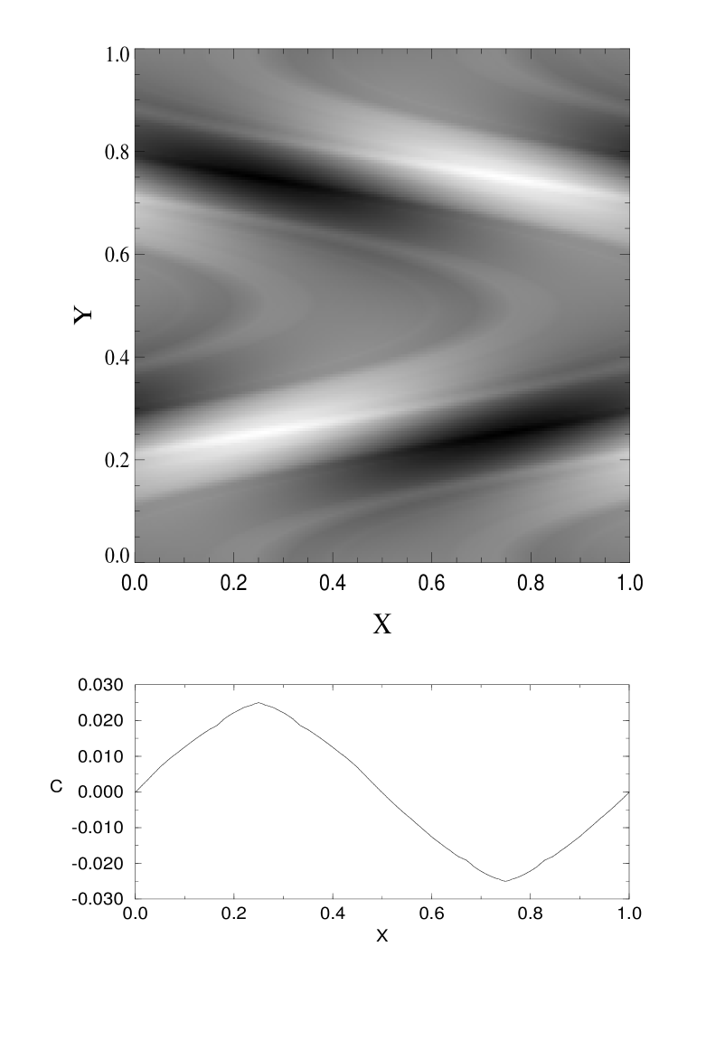
FIG. 1.: Top: a snapshot of the chemical concentration $C_{\infty}$ obtained for $b=4.0$ and $\lambda=2.67$, so that a smooth distribution is obtained. Bottom: a horizontal cut along the line $y=0.25$.

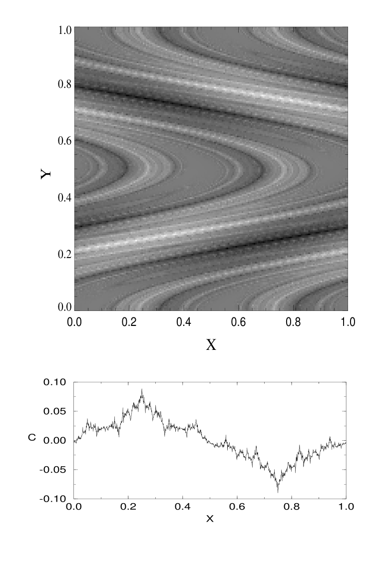
FIG. 2.: Top: a snapshot of the chemical concentration $C_{\infty}$ for $b=0.1$ and $\lambda=2.67$, so that a filamental structure is obtained. The lower panel shows a horizontal cut along the line $y=0.25$, clearly displaying the fractal nature of the field.

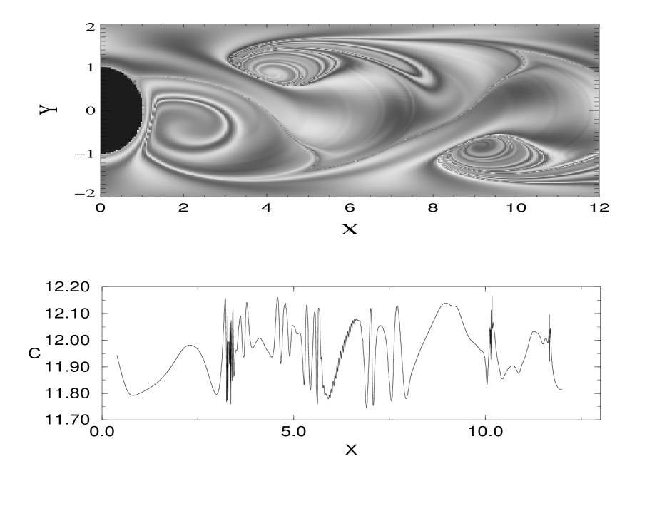
FIG. 3.: Top: a snapshot of the chemical pattern $C_{\infty}$ formed in the wake of a cylinder (the black semicircle at the left is half of its section). Mean flow is from left to right. We have used the streamfunction given in reference [15]. $b=0.96$, and all the streamfunction parameter values are the same as in [15] except the boundary-layer thickness of the cylinder which here takes the value $a=20.0$, and the vorticity strength which is $\omega=35.06$ in our calculations. Bottom: a horizontal cut taken along the line $y=1.0$.

FIG. 4.: Top: The absolute value of the gradient of the chemical field in Fig. 3 along the line $x=7.3$. The lower figure shows the escape time for particles along this line ($x=7.3$). This is calculated by computing the time that every single particle takes to arrive to the line $x=-2.0$ (far from the chaotic wake region) in the backwards-in-time dynamics.

FIG. 5.: The distribution of finite-time Lyapunov exponents at three different times, obtained for the closed flow (22) with $T=1.0$ and $U=1.2$. The long-time mean Lyapunov exponent is $\lambda_{0}=2.67$.

FIG. 6.: The function $G(\lambda)$, obtained from the distributions in Fig. 5 and Eq. (32). Collapse of data for the three times into the same curve confirms the validity of (32). The dotted line is a parabolic fit ($0.4(\lambda-2.67)^{2}$) that provides a good approximation near the minimum.

FIG. 7.: The scaling exponents $\zeta_{q}$ for the situation of Figs. 5 and 6 and with $b=1.0$. Thick line: the mono-fractal approximation $\zeta_{q}=qb/\lambda_{0}$. Thin lines: the curves $\zeta_{q}=q$ and $\zeta_{q}=[qb+G(\lambda)]/\lambda$, for different values of $\lambda$; the numerical values of $G(\lambda)$ are obtained from Fig. 6. According to Eq. (38), the actual values of the scaling exponents are given by the lower envelope of this set of curves. This is confirmed by the numerically determined values of $\zeta_{q}$ (crosses). Dashed line: the approximation (42).

- [1] J.M. Ottino, The Kinematics of Mixing: Stretching, Chaos, and Transport (Cambridge Univ. Press, Cambridge, 1989).
- [2] H. Aref, J. Fluid Mech. 143, 1 (1984); J.H.E. Cartwright, M. Feingold, and O. Piro in Mixing: Chaos and Turbulence, H. Chaté and E. Villermaux Eds. (Kluwer, Dordretch, 1999).
- [3] I.R. Epstein, Nature 374, 321 (1995).
- [4] S. Edouard, B. Legras, F. Lefèvre and R. Eymard, Nature, 384, 444 (1996).
- [5] C. Marguerit, D. Schertzer, F. Schmmitt, S. Lovejoy, J. Mar. Sys. 16, 69 (1998).
- [6] G. Metcalfe and J.M. Ottino, Phys. Rev. Lett. 72, 2875 (1994).
- [7] Z. Toroczkai, Gy. Károlyi, Á. Péntek, T. Tél and C. Grebogi, Phys. Rev. Lett. 80, 500 (1998); Gy. Károlyi, Á. Péntek, Z. Toroczkai, T. Tél, and C. Grebogi, Phys. Rev. E 59, 5468 (1999).
- [8] Z. Neufeld, C. López and P.H. Haynes, Phys. Rev. Lett. 82, 2606 (1999). chao-dyn/9906019
- [9] J.-P. Eckmann and D. Ruelle, Rev. Mod. Phys. 57, 617 (1985).
- [10] E. Abraham, A note on the wavenumber spectra of sea-surface temperature and chlorophyll, preprint (1999).
- [11] C. López, Z. Neufeld, E. Hernández-García, P.H. Haynes, Chaotic advection of reacting substances: Plankton dynamics on a meandering jet, preprint chao-dyn/9906029.
- [12] E. Ott, Chaos in Dynamical Systems (Cambridge Univ. Press, Cambridge, 1993).
- [13] T. Tél, in Directions in Chaos, Vol. 3, edited by Hao Bai-Lin (World Scientific, Singapore, 1990).
- [14] E. Ziemniak, C. Jung and T. Tél, Physica D 76, 123 (1994)
- [15] C. Jung, T. Tél and E. Ziemniak, CHAOS 3, 555 (1993).
- [16] J.C. Sommerer, H.-C. Ku and H.E. Gilreath, Phys. Rev. Lett. 77, 5055 (1996).
- [17] T. Bohr, M. Jensen, G. Paladin, A. Vulpiani, Dynamical Systems Approach to Turbulence (Cambridge Univ. Press, Cambridge, 1998).
- [18] K. Nam et al., The k spectrum of finite lifetime passive scalar in Lagrangian chaotic fluid flows, (preprint, 1999).
- [19] T. Antonsen, Jr. Z. F. Fan and E. Ott, Phys. Rev. Lett., 75, 1751 (1995).
- [20] M. Chertkov, Phys. Fluids 10, 3017 (1998). chao-dyn/9803007.
- [21] E. Ott, T. M. Antonsen, Jr., Phys. Rev. Lett. 61, 2839 (1988).
- [22] T. M. Antonsen, Jr. and E. Ott, Phys. Rev. A, 44, 851 (1991)
- [23] M. Falcioni, G. Paladin and A. Vulpiani, Phys. Rev. Lett., 64, 698 (1990); E. Ott, T.M. Antonsen Jr., Phys. Rev. Lett., 64, 699 (1990).
- [24] G.-C. Yuan et al., Power spectrum of passive scalars in two-dimensional chaotic flows (preprint, 1999).
- [25] J. Bacmeister et al., in Gravity wave processes, edited by K. Hamilton (Springer-Verlag, New York, 1997).
- [26] A.F. Tuck and S.J. Hovde, Geophys. Res. Lett. (1999, to appear).
- [27] L. Seuront, F. Schmitt, Y. Lagadeuc, D. Schertzer, S. Lovejoy and S. Frontier, Geophys. Res. Lett. 23, 3591 (1996).