Synchronization of chaotic oscillations in doped fiber ring lasers

Abstract

We investigate synchronization of and subsequently communication using chaotic rare-earth-doped fiber ring lasers, represented by a physically realistic model introduced in [4]. The lasers are first coupled by transmitting a fraction $c$ of the circulating electric field $\mbox{$\bf{E}$}_{T}$ in the transmitter and injecting it into the optical cavity of the receiver, e.g., by fiber optics. We then analyze a coupling strategy which relies on modulation of the intensity of the light alone. This avoids problems associated with polarization and phase of the laser light.

We study synchronization as a function of the coupling strength and see excellent convergence, even with small coupling constants. We prove that in an open loop configuration ($c=1$) synchronization is guaranteed due to the particular structure of our equations and of the injection method we use for these coupled laser systems [5].

We also analyze the generalized synchronization of these model lasers when there is parameter mismatch between the transmitter and the receiver. The synchronization is insensitive to a wide range of mismatch in laser parameters, including the pumping level and the gain in the active medium, but it is sensitive to other parameters, in particular those associated with the phase and the polarization of the circulating electric field, and the lengths of the passive fiber rings. Less restrictive synchronization metrics reduce the sensitivity to mismatch.

We then address communicating information between the transmitter and receiver lasers. We investigate a scheme for modulating information onto the chaotic electric field and demodulation and detection of the information embedded in the chaotic signal passing down the communications channel. The modulation scheme consists of an invertible operation in which the message to be transmitted, raised from its baseband status to the optical passband, is combined with the light in the transmitter. At the receiver, we invert the combining operation and recover the message.

Many of the ideas we consider have been demonstrated experimentally by Roy and VanWiggeren [6, 7, 8]. Their remarkable experimental success at high symbol rates and low bit error rates attests to the viability of the communications methods we investigate here.

Finally we comment on the cryptographic setting of our algorithms, especially the open loop strategy at $c=1$, and hope this may lead others to perform the cryptographic analyses to determine which, if any, of the communications strategies we investigate are secure. At $c=1$ our methods are known in the cryptographic literature as self-synchronous stream ciphers operating in cipher feedback mode. For $c\neq 1$, ours is a type of cryptographic system apparently not known in that field. Neither a cryptanalysis nor any claims for security of communication are made here.

Contents

toc

I Introduction

Synchronization of chaotic oscillators is a phenomenon found quite often in physical and biological systems. The idea that chaotic systems could synchronize their motions was suggested some time ago by Fujisaka and Yamada [9] and independently by Afraimovich, Rabinovich and Verichev [10]. An early investigation of synchronization in neural networks [11] explored application in a wider arena.

The idea was again independently proposed and then experimentally explored by Pecora and Carroll [12]. The latter authors also suggested that the use of synchronized chaotic oscillators for communications would be of some interest. The work of Pecora and Carroll led to the investigation of a wide variety of synchronized chaotic systems [13] including close relatives of those we discuss in this paper.

In this paper we explore the synchronization properties of the models we have built for rare-earth-doped fiber ring lasers (DFRLs) [4]. Our plan here is to use two such model lasers connecting them by transmitting the electric field $\mbox{$\bf{E}$}_{T}$ circulating in one laser (the transmitter) to a second identical laser (the receiver). Into the optical cavity of the receiver laser we re-inject a fraction $(1-c)\mbox{$\bf{E}$}_{R}$ of the receiver field $\mbox{$\bf{E}$}_{R}$ and also add a fraction $c\mbox{$\bf{E}$}_{T}$ of the field arriving from the first laser. The net field entering the receiver laser is then $c\mbox{$\bf{E}$}_{T}+(1-c)\mbox{$\bf{E}$}_{R}$. This setup is sketched in Fig. 1. When the lasers are synchronized so that $\mbox{$\bf{E}$}_{R}=\mbox{$\bf{E}$}_{T}$, then the combination $c\mbox{$\bf{E}$}_{T}+(1-c)\mbox{$\bf{E}$}_{R}$ is independent of c and equal to the field in either laser. As we vary c, we change the precise combination of transmitter field and receiver field which is seen at the receiver.

We investigate the synchronization both for identical transmitter and receiver, and then for lasers which have various parameter mismatches including the gain and pumping of the active medium, their polarization characteristics, and their ring length. The synchronization is quite robust for mismatches in gain and pumping power, but it is very sensitive to mismatches in polarization or phase characteristics of the transmitter and receiver. This is shown in some detail, and the origin of the loss of synchronization is analyzed.

Because of this sensitivity, we investigate another coupling strategy which uses only the intensity of the circulating electric fields to connect the transmitter and receiver. This is shown to be a potentially viable method of synchronizing the lasers, and an example of communicating using amplitude modulation of the transmitter intensity is investigated.

Many of the papers on synchronization of chaotic systems have dealt with applications to communications. While we are focused here on the use of doped fiber ring lasers, the principles associated with synchronization and communication are shared by earlier investigations, in particular at $c=1$ by the methods of Rulkov and Volkovskii [14] and those of Kocarev and Parlitz [15].

The attraction of using chaotic signals as the carriers of information comes from their potentially efficient use of channel bandwidth as well as the low cost and power efficiency of some chaotic transmitters and receivers [16]. There has also been much discussion of the security of communications systems based on chaotic carriers. The security of any such system depends in detail of the modulation methods used, not on the perception that the carrier is complex or temporally irregular. Whether any given modulation/demodulation strategy is secure needs to be determined by a rigorous cryptographic analysis, and in this paper we do not discuss this issue or attempt to provide such an analysis. We do comment in this paper on the cryptographic setting of our methods at $c=1$ where similar algorithmic structures using linear shift registers have been known and subjected to cryptographic scrutiny. When the transmitter and receiver are synchronized, but the receiver is not run open loop ($c\neq 1$), we know of no systematic analysis for such systems in the same general cryptographic framework. This may be a new class of systems. We hope that this paper and others in this area will stimulate research into these issues and provide guidelines for design of secure chaotic communications systems, when they are desired.

II Equations for an Individual DFRL

We use the model introduced in [4]. The doped fiber ring laser (DFRL) we consider contains an optical amplifier composed of rare-earth-doped single-mode fiber of length $l_{A}$, whose active atoms are pumped by an external laser diode source. Connecting the output of this active section to its input is a piece of passive fiber of length $l_{F}$. In the passive fiber is an isolator which guarantees the direction of flow of light, a polarization controller, and a location where external light of given amplitude and frequency $\omega_{I}$ can be injected into the fiber. The total length of the fiber cavity is $L=l_{A}+l_{F}$. The general locations of the relevant parameters for each laser is shown schematically in Fig. 2.

The electric fields $\mbox{$\bf{E}$}(z,t)$ are described by the envelope $\mbox{{$\cal E$}}(z,t)$ of the optical plane wave of frequency $\omega_{0}$, $\mbox{$\bf{E}$}(z,t)=\mbox{{$\cal E$}}(z,t)e^{i(k_{0}z-\omega_{0}t)}$ where $\omega_{0}=k_{0}c/n$. The dynamics of $\mbox{{$\cal E$}}(z,t)$ consists

• of linear birefringence of magnitude

  $$\Delta=n_{0}(n_{x}-n_{y}),$$ (1)

  where $n_{x}$ and $n_{y}$ are the indices of refraction along the principal axes of the fiber, and $n_{0}=(n_{x}+n_{y})/2$,

• of group velocity dispersion (GVD) which comes from second order variations in frequency of the linear dispersion relation of the fiber,

• of contributions to the polarization of the medium associated with the population inversion of the atomic levels, and

• of nonlinear polarization effects associated with the Kerr term cubic in electric field strength.

With these effects included, our equations for the propagation of the electric field envelope $\mbox{{$\cal E$}}=(\mbox{{$\cal E$}}_{x},\mbox{{$\cal E$}}_{y})$ in the active medium $0\leq z\leq l_{A}$ become, in retarded coordinates $z=z,\tau=t-z/v_{g}$ with $v_{g}$ is the group velocity of the waves,

$$\frac{\mbox{$\partial$}\mbox{{$\cal E$}}_{x,y}(z,\tau)}{\mbox{$\partial$}z}=gn(\tau)\mbox{{$\cal E$}}_{x,y}+\mbox{{\bf L}}_{x,y}\mbox{{$\cal E$}}_{x,y}+\mbox{{\bf N}}_{x,y}\mbox{{$\cal E$}}_{x,y}.$$ (2)

L contains the linear parts of the propagation operator excluding gain, and N the Kerr nonlinearity. The linear operator L, including birefringence, GVD and gain dispersion, is most naturally represented in the Fourier domain:

$$\mbox{{\bf L}}_{x,y}=\pm\frac{ik_{0}(n_{x}-n_{y})}{2n_{0}}\mp\frac{\Delta}{n_{0}c}i\mbox{$\omega$}-\frac{i}{2}\beta_{2}\mbox{$\omega$}^{2}-\frac{gn(\tau)\mbox{$\omega$}^{2}T_{2}^{2}}{1+\mbox{$\omega$}^{2}T_{2}^{2}}$$ (3)

with $\omega$ the signal angular frequency. The first term in $\mbox{{\bf L}}_{x,y}$ only results in an overall arbitrary phase shift for the two polarizations, which can be absorbed without loss of generality into the parameterization of the passive section described below. The term linear in $\omega$ represents linear birefringence; the next term, quadratic in $\omega$, is the group velocity dispersion. The last term is associated with the gain curve, and arises from the fact that the center frequency of the line $\mbox{$\omega$}=0$ is amplified more strongly than frequencies on either side of the line. The nonlinear operators are

$$\mbox{{\bf N}}_{x}\mbox{{$\cal E$}}_{x} = i\chi_{3}\biggl{\{}\left(|\mbox{{$\cal E$}}_{x}(z,\tau)|^{2}+\frac{2}{3}|\mbox{{$\cal E$}}_{y}(z,\tau)|^{2}\right)\mbox{{$\cal E$}}_{x}(z,\tau)+\frac{1}{3}\mbox{{$\cal E$}}_{x}^{*}(z,\tau)\mbox{{$\cal E$}}_{y}(z,\tau)^{2}\biggr{\}}$$ (4)

$$\mbox{{\bf N}}_{y}\mbox{{$\cal E$}}_{y} = i\chi_{3}\biggl{\{}\left(|\mbox{{$\cal E$}}_{y}(z,\tau)|^{2}+\frac{2}{3}|\mbox{{$\cal E$}}_{x}(z,\tau)|^{2}\right)\mbox{{$\cal E$}}_{y}(z,\tau)+\frac{1}{3}\mbox{{$\cal E$}}_{y}^{*}(z,\tau)\mbox{{$\cal E$}}_{x}(z,\tau)^{2}\biggr{\}}.$$ (5)

The physical implication of this third-order nonlinearity is most easily characterized by the non-dimensional phase shift $\Phi_{nl}$ experienced by an $\cal E$ field as it passes through the fiber given by [17]

$$\Phi_{nl}=\frac{\chi_{3}\pi L}{\lambda}(P_{a}+2P_{b}),$$ (6)

where $P_{a}$, $P_{b}$ are the optical powers in the parallel and perpendicular direction. We parameterize our simulations by $\Phi_{nl}$ and vary its value to tune in a desired amount of optical nonlinearity. Physically this could be interpreted as changing various parameters such as active medium pumping, which would increase the optical power, or changing the value of the ring fiber length L.

These equations must be solved numerically to propagate the light from its entry into the doped fiber amplifier (DFA) at $z=0$ to its exit at $z=l_{A}$, represented here by a propagation operator on the vector $\mbox{{$\cal E$}}=\left[\mbox{{$\cal E$}}_{x},\mbox{{$\cal E$}}_{y}\right]$: $\mbox{{$\cal E$}}(z=l_{A},t+l_{A}/v)=\mbox{\sf P}\{\mbox{{$\cal E$}}(z=0,t)\}$.

The polarization of the electric field in the ring is affected by the birefringence in the fiber arising from numerous small effects associated with imperfections in the fiber, strains, etc. Following [18] we write the net effect of the fiber on the polarization states of the field as a unitary Jones matrix which we call $\mbox{$\bf{U}$}_{\mbox{Whole Fiber}}$.

The overall propagation map including all the passive parts of the ring and external injection is,

$$\mbox{{$\cal E$}}(t+\tau_{R})=\mbox{{$\cal A$}}(t+\tau_{R})e^{i(\omega_{I}-\omega_{0})(t+\tau_{R})}+\biggl{(}\mbox{{\bf R}}\mbox{$\bf{J}$}_{PC}\mbox{$\bf{U}$}_{\mbox{Whole Fiber}}\biggr{)}\mbox{\sf P}\{\mbox{{$\cal E$}}(t)\}.$$ (7)

Reading from left to right the terms are external monochromatic injection, possibly polarization dependent attenuation, $\mbox{{\bf R}}=\mbox{diag}(R_{x},R_{y})$, the unitary Jones matrix for the polarization controller $\mbox{$\bf{J}$}_{PC}$, the matrix for the passive fiber, and the propagator through the active medium. This discrete-time map, a recursion relation between the field at a time $t$ and at a time $\tau_{R}$ later, is one of the dynamical rules of our ring laser system. The other is the population inversion equation in its simplified form.

The physics of the atomic polarization in the active medium is governed by the usual Bloch equation for the population inversion at time $\tau$ and spatial location z:

$$\frac{\mbox{$\partial$}n(z,\tau)}{\mbox{$\partial$}\tau}=Q-\frac{1}{T_{1}}(n(z,\tau)+1)-\xi n(z,\tau)|\mbox{{$\cal E$}}(z,\tau)|^{2},$$ (8)

with $Q$ pumping, $T_{1}$ the lifetime of the excited state (10 ms for a typical erbium-doped fiber) and $\xi$ a constant relating to the optical cross section governing the transition rate between levels. Assuming $g$ real, we can integrate (8) by ${l_{A}}^{-1}\int_{0}^{l_{A}}dz$ to arrive at the dynamics for the population inversion averaged over the entire active medium $w(\tau)={l_{A}}^{-1}\int_{0}^{l_{A}}dz\,n(z,\tau)$

$$\frac{dw(\tau)}{d\tau}=Q-\gamma\left(w(\tau)+1+\left(e^{2l_{A}gw(\tau)}-1\right)|\mbox{{$\cal E$}}(z=0,\tau)|^{2}\right),$$ (9)

where $\gamma$ is the ratio of round trip time to excited state lifetime, $\tau_{R}/T_{1}$.

It is important to note that, except for the gain term, the magnitude $|\mbox{{$\cal E$}}|^{2}$ is preserved by our propagation operations including the nonlinear Kerr phase shifts. After the Kerr operator, the main component of the gain is applied to the two complex envelopes, multiplying each by $\exp(gl_{A}w(\tau))$, and finally, the passive components of the ring, to produce $\mbox{{$\cal E$}}_{x,y}(t+\tau_{R})$.

Potentially, there is a third dynamical equation associated with the evolution of the polarization of the medium through which the electric field passes. The time constant, usually called $T_{2}$, for this process is about a picosecond, thus we have safely eliminated that equation and used the resulting “static” polarization in the population inversion equation. This is known as a “class B” laser.

We summarize the equations for use below as a map $\mbox{\bf M}_{\mbox{{$\cal E$}}}(w(\tau),\mbox{{$\cal E$}}(\tau))$ of the electric field from time t to time t+$\tau_{R}$ and a differential equation for the integrated population inversion:

$$\mbox{{$\cal E$}}(\tau+\tau_{R}) = \mbox{\bf M}_{\mbox{{$\cal E$}}}(w(\tau),\mbox{{$\cal E$}}(\tau))$$ (10)

$$\frac{dw(\tau)}{d\tau} = Q-\gamma\biggl{\{}w(\tau)+1+|\mbox{{$\cal E$}}(\tau)|^{2}(e^{Gw(\tau)}-1)\biggr{\}},$$ (11)

where the active medium specific overall gain term $G$ is defined as $G=2l_{A}g$.

The details of our numerical schemes are to be found in our earlier paper [4]. Straightforward integration of the partial differential equations at a resolution sufficient to capture complex sub-round trip dynamics as seen in experiment results in an algorithm which is far too slow. We implemented a scheme which can integrate a whole round trip at a time, combined with a buffering method to process the portion of the linear operator in the Fourier domain. Even still, computation takes approximately 18 hours on a contemporary workstation to achieve equilibrium (500,000 round trips) on account of the very large difference in time scales between the fluorescence lifetime $T_{1}\approx 10$ ms associated with an erbium doped fiber and the time resolution of our simulation $\delta t\approx 80$ ps, necessary to capture the high frequency dynamics seen in experiment and thus high-bandwidth communication.

III Synchronization of Two DFRLs

We now construct a transmitter and receiver pair and couple their electric fields by an optical channel. First we examine the synchronization of two identical lasers. Next we investigate the robustness of this synchronization as the transmitter and receiver are mismatched in various of the physical parameters of the model. We then look at the robustness of the synchronization against noise in the communication channel between transmitter and receiver. This will lead us into considerations of generalized synchronization of the two optical oscillators. Finally, we suggest an alternate coupling scheme and synchronization method constructed to avoid some of the experimental problems typically encountered with direct optical coupling.

The values of the model parameters associated with the experiments of Van Wiggeren and Roy [7, 8] used for the group of simulations in this paper are listed in table I. The model with these parameters produces chaotic waveforms with a largest Lyapunov exponent, evaluated with the numerical procedure of [4]: $\mbox{$\lambda$}_{1}=(6.3\pm 0.3)\times 10^{3}/s$.

A Identical Transmitter and Receiver

In our study of the synchronization of two EDFRLs we have a transmitter laser with dynamical variables $\mbox{{$\cal E$}}_{T}(t)$ and $n_{T}(t)$ and a receiver laser with $\mbox{{$\cal E$}}_{R}(t)$ and $n_{R}(t)$. The two lasers are started in different initial conditions, allowed to run several hundred thousand round trip times uncoupled to reach their asymptotic state. Coupling is then activated. The transmitter’s field $\mbox{{$\cal E$}}_{T}(t)$ is then injected into the receiver laser multiplied by a factor $c$ while the circulating electric field in the receiver is attenuated by a factor $1-c$, and both are optically recombined before entering the rare-earth-doped amplifier section of the laser ring. The nonlinear amplifying element receives $c\mbox{{$\cal E$}}_{T}(t)+(1-c)\mbox{{$\cal E$}}_{R}(t)$ as its input. When the transmitter and receiver are synchronized, so $\mbox{{$\cal E$}}_{T}(t)=\mbox{{$\cal E$}}_{R}(t)$, the linear combination $c\mbox{{$\cal E$}}_{T}(t)+(1-c)\mbox{{$\cal E$}}_{R}(t)=\mbox{{$\cal E$}}_{R}(t)=\mbox{{$\cal E$}}_{T}(t)$ is a solution to the equations of motion for each laser. This setup is illustrated in Fig. 1. This kind of coupling is experimentally achievable with standard fiber optic equipment.

The equations for this unidirectional coupling between the chaotic systems are for the transmitter

$$\mbox{{$\cal E$}}_{T}(\tau+\tau_{R}) = \mbox{\bf M}_{\mbox{{$\cal E$}}}(w_{T}(\tau),\mbox{{$\cal E$}}_{T}(\tau))$$ (12)

$$\frac{dw_{T}(\tau)}{d\tau} = Q-\gamma\biggl{\{}w_{T}(\tau)+1+|\mbox{{$\cal E$}}_{T}(\tau)|^{2}(e^{Gw_{T}(\tau)}-1)\biggr{\}},$$ (13)

and for the receiver

$$\mbox{{$\cal E$}}_{R}(\tau+\tau_{R}) = \mbox{\bf M}_{\mbox{{$\cal E$}}}(w_{R}(\tau),c\mbox{{$\cal E$}}_{T}(\tau)+(1-c)\mbox{{$\cal E$}}_{R}(\tau))$$ (14)

$$\frac{dw_{R}(\tau)}{d\tau} = Q-\gamma\biggl{\{}w_{R}(\tau)+1+|c\mbox{{$\cal E$}}_{T}(\tau)+(1-c)\mbox{{$\cal E$}}_{R}(\tau)|^{2}(e^{Gw_{R}(\tau)}-1)\biggr{\}}.$$ (15)

When $c=0$, the lasers are uncoupled and run independently. If all of the physical parameters in the two laser subsystems are identical, the electric field in each laser visits the same attractor. $\mbox{{$\cal E$}}_{T}(t)$ and $\mbox{{$\cal E$}}_{R}(t)$ as well as $n_{T}(t)$ and $n_{R}(t)$ are uncorrelated due to the instabilities in the phase space of the system. As we increase $c$ away from zero, we anticipate that for a certain minimum coupling, the lasers will asymptotically achieve identical synchronization, $\mbox{{$\cal E$}}_{T}(t)=\mbox{{$\cal E$}}_{R}(t)$, and $n_{T}(t)=n_{R}(t)$, even though the population inversions are not physically coupled. To exhibit this we run the two systems for the order of $10^{4}$ round trips following their coupling. First, we ask after what time the quantity

$$H_{E}(c,t)=\frac{|\mbox{{$\cal E$}}_{T}(t)-\mbox{{$\cal E$}}_{R}(c,t)|}{{\langle|\mbox{{$\cal E$}}_{T}|\rangle}_{\tau_{R}}},$$ (16)

becomes and remains less than some small number. The denominator is the average of $\mbox{{$\cal E$}}_{T}(t)$ taken over the round trip previous to coupling and gives a convenient normalization for the magnitude of the synchronization error $H_{E}(c,t)$. An EDFRL possesses the property that after the effects of initial transients, the laser achieves a constant mean intensity per round trip even though the waveform is chaotic. In our simulation, the lasers were run long enough before coupling for the transients to damp out, so in $H_{E}(c,t)$ the value of ${\langle|\mbox{{$\cal E$}}_{T}(t)|\rangle}_{\tau_{R}}$ is approximately constant in the transmitter from round trip to round trip.

The time to synchronization $\tau_{s}$ is selected so at $t=\tau_{s}$ the synchronization error $H_{E}(c,t)$ becomes less than some small value $\epsilon$, and then stays smaller than $\epsilon$ for all times $t>\tau_{s}$. Choosing $\epsilon=10^{-2}$, we plot $\tau_{s}$ in Figure 3 as a function of $c$ for $0\leq c\leq 1$. We see that for some values of $c\leq 0.1$, the lasers do synchronize, but it takes nearly $100\mu$s to come within $\epsilon$. This is much longer than when $c\geq 0.2$, however, where synchronization sets in rapidly ($\tau_{s}\leq 5\mu$s). This figure represents the average time to synchronization over 25 different initial conditions for each system, thus substantially reducing the effect of individual trajectory behavior. One lesson we can draw from Figure 3 is that at $c=1$, which is open loop operation of the receiver, synchronization within $\epsilon$ sets in essentially instantaneously.

This $\tau_{s}$ is the time at which the synchronization error $H_{E}(c,t)$ falls below an arbitrary specified level. This measure reveals little about the synchronization dynamics beyond this time. We now examine the residual synchronization error $H_{E}(c,t)$ for large times after coupling. We adopt the general unifying definition of synchronization proposed by Brown and Kocarev [19]. Their formalism states that two subsystems are synchronized with respect to the subsystem properties $g(x)$ and $g(y)$, if there is a time-independent function $h$, such that

$$||h[g(x),g(y)]||=0,$$ (17)

where $||\bullet||$ is some norm. The quantities $g(x)$ and $g(y)$ are completely general and can refer to any measurable property of the subsystem. The general form of the time-independent function $h$ which we adopt here is

$$h[g(x),g(y)]\equiv\mathop{\lim}_{T\rightarrow\infty}\frac{1}{T}\int^{t+T}_{t}\left|g(x(s))-g(y(s))\right|ds.$$ (18)

For practical reasons, we must modify this statement somewhat, since numerically we can neither take $T\rightarrow\infty$, nor hope for $||h[g(x),g(y)]||$ to equal precisely zero, since we will reach the numerical limits of computation before that occurs.

To keep in the spirit of this definition, we let the coupled chaotic lasers run for K round trips after coupling, then calculate the RMS value of $H_{E}(c,t)$ over M additional round trips to examine the magnitude of the synchronization error for large times after coupling. This leads us to the synchronization error function

$$D_{E}(c)=\frac{1}{\mbox{{$\cal N$}}_{E}}\left(\int_{K\tau_{R}}^{(K+M)\tau_{R}}H_{E}^{2}(c,t)dt\right)^{1/2}.$$ (19)

The normalization factor $\mbox{{$\cal N$}}_{E}$ is the RMS average for the $c=0$ or uncoupled case

$$\mbox{{$\cal N$}}_{E}=\left(\int_{K\tau_{R}}^{(K+M)\tau_{R}}H_{E}^{2}(c=0,t)dt\right)^{1/2}$$ (20)

and is included to give us a tangible measure of the magnitude of the synchronization error at $c$ versus the case of no coupling, $c=0$. This function compares directly the difference of fields in the coupled lasers, so for us $g(x)$ and $g(y)$ in equation (18) are

$$g(x(t)) = \frac{\mbox{{$\cal E$}}_{T}(t)}{{\langle|\mbox{{$\cal E$}}_{T}|\rangle}_{\tau_{R}}}$$ (21)

$$g(y(t)) = \frac{\mbox{{$\cal E$}}_{R}(c,t)}{{\langle|\mbox{{$\cal E$}}_{T}|\rangle}_{\tau_{R}}}.$$ (22)

In the work we report here we used $K=20,000$ and $M=3,000$.

Fig. 4 displays the synchronization error function $\log_{10}[D_{E}(c)]$ versus $c$. We see a quite different picture of the synchronization here. Above we noted that for coupling as low as $c=0.1$, the lasers took a much longer time ($\approx 0.1$ ms) than for higher coupling for $H_{E}(c,t)$ to become as small as $\epsilon$. However, on the time scale of a few milliseconds, we see that with much smaller coupling the synchronization error $D_{E}(c)$ is less by many orders of magnitude. Note, however, that the error never exceeds a few parts in $10^{7}$ for any $c$. Once the lasers synchronize at some $c$, they do so very accurately.

To investigate these results quantitatively, we look at a plot which shows the temporal behavior of the synchronization error $D_{E}(c)$. We reintroduce a discrete time variable $N\tau_{R}$, where $N$ is the number of round trips since coupling was initiated, and $\tau_{R}$ is the round trip time. We then define $D_{E}(c,N)$ as the synchronization error averaged over a round trip

$$D_{E}(c,N)=\frac{1}{\mbox{{$\cal N$}}_{E}}\left(\int_{(N-1)\tau_{R}}^{N\tau_{R}}H_{E}^{2}(c,t)dt\right)^{1/2}.$$ (23)

Fig. 5 shows the evolution of $\ln(D_{E}(c,N))$ versus $N$ for couplings in the range $0.01\leq c\leq 1.0$. We see a pattern in convergence rates with varying coupling (the rate of convergence is the slope of the $\ln(D_{E})-N$ plot). After an initial rapid jump of $D_{E}(c,N)$ towards synchronization in the first few round trips, the weaker coupling cases converge at an increasingly faster rate (they have steeper negative slopes), with the slowest convergence rate occurring at the strongest coupling, $c=1$.

There are thus two time scales of synchronization. There is an initial time scale ($t<1\mu$s) with a rapid, short term convergence toward synchronization, then slower convergence rate for longer times ($t>1\mu$s). For weaker coupling, the initial convergence of the lasers is not as large as for the stronger coupling case, since the amount of optical field from the transmitter being introduced into the receiver is proportional to the coupling strength. However, past this initial short time scale, the weaker coupling draws together the two lasers’ trajectories at a faster rate than for the stronger coupling.

Examining the weak coupling range, $0.01\leq c\leq 0.04$ in Fig. 5, we see that the magnitude of the convergence rate is maximal between $0.02\leq c\leq 0.04$. Figure 6 shows the rate of convergence plotted against coupling constant c. The coupling is linear in $\mbox{{$\cal E$}}_{T}(t)$ and $\mbox{{$\cal E$}}_{R}(t)$, so this complex synchronization behavior is not likely due to this mixing of the optical fields alone, therefore we look for explanations outside of the optical field variables. The other system variables are the population inversions $w_{T}(t)$ and $w_{R}(t)$. They cannot be directly coupled, being related only indirectly through the nonlinear relationship to their respective internal optical intensities (equation (9)).

The time dependence of $w_{R}(t)$ and $w_{T}(t)$ reveals insight into the dynamics just after the lasers are coupled. In Fig. 7 we show $w_{R}(t)-w_{T}(t)$ as a function of time after the lasers are coupled and as a function of $c$. In the transmitter, $w_{T}(t)$, is essentially constant because erbium’s fluorescence lifetime $T_{1}$ is so long ($T_{1}\approx\,$ 10 ms) so that in the long-term asymptotic state of the laser, changes in $w_{T}(t)$ occur only on the order of $10^{5}$ round trips. There is always a rise in $w_{R}(t)$ immediately after coupling because when $0<c<1$, the intensity in the receiver laser just as the lasers are coupled is $|c\mbox{{$\cal E$}}_{T}|^{2}+|(1-c)\mbox{{$\cal E$}}_{R}|^{2}+2c(1-c)\mbox{\,Re\,}(\mbox{{$\cal E$}}_{T}\cdot\mbox{{$\cal E$}}_{R}^{*})$ averaged over a round trip, and the cross term averages to zero since the fields are initially uncorrelated. As ${\langle|\mbox{{$\cal E$}}_{T}|^{2}\rangle}$ and ${\langle|\mbox{{$\cal E$}}_{R}|^{2}\rangle}$ averaged over a round trip are equal, the average intensity initially entering the receiver’s active medium will be less that ${\langle|\mbox{{$\cal E$}}_{R}|^{2}\rangle}$ by a factor of $c^{2}+(1-c)^{2};\;1/2\leq c^{2}+(1-c)^{2}\leq 1$. This allows the pumping term to increase the receiver population inversion as the active medium sees a reduced intensity trying to stimulate transitions between lasing states.

This effect continues only as long as $\mbox{\,Re\,}(\mbox{{$\cal E$}}_{T}\cdot\mbox{{$\cal E$}}_{R}^{*})\ll|\mbox{{$\cal E$}}_{T}||\mbox{{$\cal E$}}_{R}|$. For large coupling, correlation of the two fields occurs within a few round trips, before the population inversion has a chance to increase much. However, for small coupling, it takes several hundred round trips for the two lasers’ fields to start becoming correlated, so the population inversion has the chance to grow substantially. This in turn will cause the average electric field intensity in the receiver laser to grow.

We see in Fig. 7 for $c=0.002$, that $w_{R}(t)$ oscillates in a manner reminiscent of an under-damped oscillator. This coupling coefficient is an order of magnitude smaller than the region we found to contain the fastest convergence rate and the figure verifies that the oscillations are slow to decay, thereby causing the approach to synchronization to also be slow. In the same figure for $c=0.01$, which is closer to the optimal coupling region, and we can see that the oscillations are still present, but are decaying much faster. As we reach the optimal convergence region at $c=0.02$, we see that the decay now takes only a little more than an oscillatory cycle to damp considerably. This would correspond to the near critically-damped case. Then as we increase coupling further to $c=0.2$, the oscillations are gone but now after the initial rise in $w_{R}(t)$, it again takes much longer to decay, much like an over-damped oscillator.

To finish the examination of the case of identical subsystems, we next determine the minimal value of $c$ which leads to synchronization. In the discussion above the lasers always synchronize, so now we examine weaker coupling yet. To do this we numerically evaluate the largest conditional Lyapunov exponent [12] in much the same way as we find the standard largest Lyapunov exponents in our earlier paper [4]. Now we couple the identical lasers with small coupling $c$ and ask when the largest conditional exponent becomes negative as we vary $c$. The critical value of coupling was found to be $c_{crit}\approx 1.3\times 10^{-3}$. Therefore, for $c<c_{crit}$, we observe no synchronization, as a positive conditional exponent implies loss of synchronization.

B Synchronization at c = 1

We analytically examine our coupled transmitter and receiver system at $c=1$, that is, when we run the receiver open loop. This is the configuration in the Georgia Tech experiments [6, 7, 8]. In this case the field injected into the receiver is just $\mbox{{$\cal E$}}_{T}(t)$ and none of the field in the receiver fiber is re-injected into the amplifier. The equations for the two coupled systems are

• For the Transmitter Laser

  $$\mbox{{$\cal E$}}_{T}(\tau+\tau_{R}) = \mbox{\bf M}_{\mbox{{$\cal E$}}}(w_{T}(\tau),\mbox{{$\cal E$}}_{T}(\tau))$$ (24)

  $$\frac{dw_{T}(\tau)}{d\tau} = Q-\gamma\biggl{\{}w_{T}(\tau)+1+|\mbox{{$\cal E$}}_{T}(\tau)|^{2}(e^{Gw_{T}(\tau)}-1)\biggr{\}}$$ (25)

• For the Receiver Laser

  $$\mbox{{$\cal E$}}_{R}(\tau+\tau_{R}) = \mbox{\bf M}_{\mbox{{$\cal E$}}}(w_{R}(\tau),\mbox{{$\cal E$}}_{T}(\tau))$$ (26)

  $$\frac{dw_{R}(\tau)}{d\tau} = Q-\gamma\biggl{\{}w_{R}(\tau)+1+|\mbox{{$\cal E$}}_{T}(\tau)|^{2}(e^{Gw_{R}(\tau)}-1)\biggr{\}},$$ (27)

where $\mbox{\bf M}_{\mbox{{$\cal E$}}}(w(\tau),\mbox{{$\cal E$}}(\tau))$ is the map defined in earlier sections. Note that in the receiver equations only $\mbox{{$\cal E$}}_{T}(\tau)$ now appears on the right hand side. Take the difference of the population inversion equations to arrive at

$$\frac{d(w_{T}(\tau)-w_{R}(\tau))}{d\tau}=-\gamma\biggl{\{}w_{T}(\tau)-w_{R}(\tau)+|\mbox{{$\cal E$}}_{T}(\tau)|^{2}e^{Gw_{R}(\tau)}(e^{G(w_{T}(\tau)-w_{R}(\tau))}-1)\biggr{\}}.$$ (28)

Noting that $e^{x}-1\geq x$, we can write the following inequality

$$\frac{d(w_{T}(\tau)-w_{R}(\tau))}{d\tau}\leq-\gamma\left(w_{T}(\tau)-w_{R}(\tau)\right)\biggl{\{}1+|\mbox{{$\cal E$}}_{T}(\tau)|^{2}e^{Gw_{R}(\tau)}\biggr{\}}.$$ (29)

This shows that $w_{T}(\tau)-w_{R}(\tau)$ goes to zero exponentially rapidly at a rate governed by $\gamma(1+|\mbox{{$\cal E$}}_{T}(\tau)|^{2}e^{Gw_{R}(\tau)})$. This result on the synchronization at $c=1$ is a global property of these laser systems. Nowhere was a linearization made about the synchronization manifold.

This value of the convergence rate to synchronization agrees within $0.1\%$ of the numerical calculation of the same convergence rate of $w_{T}(\tau)-w_{R}(\tau)$ at $c=1$ in our numerical simulations. This gives us additional confidence in both the simulations and in the details of the approximations which went into evaluating the propagation of light around the fiber ring with nonlinear effects [4].

The final step is to use this bounded behavior of the difference in population inversions in the maps

$$\mbox{{$\cal E$}}_{T}(\tau+\tau_{R}) = \mbox{\bf M}_{\mbox{{$\cal E$}}}(w_{T}(\tau),\mbox{{$\cal E$}}_{T}(\tau))$$ (30)

$$\mbox{{$\cal E$}}_{R}(\tau+\tau_{R}) = \mbox{\bf M}_{\mbox{{$\cal E$}}}(w_{R}(\tau),\mbox{{$\cal E$}}_{T}(\tau)).$$ (31)

With this one easily shows that as $w_{T}(\tau)-w_{R}(\tau)\to 0$ so does $\mbox{{$\cal E$}}_{T}(\tau)-\mbox{{$\cal E$}}_{R}(\tau)\to 0.$ This result demonstrates global stability of the synchronization manifold $w_{T}(\tau)=w_{R}(\tau)$ as it involves no linearization of the equations around this solution. It is the detailed structure of the DFRL equations which permits this demonstration of global stability of the synchronization manifold.

The strong rate of convergence of $w_{T}(\tau)-w_{R}(\tau)$, approximately as $\exp(-\gamma|\mbox{{$\cal E$}}_{T}|^{2}\tau),$ implies that small perturbations to synchronization which might arise due to noise in the channel or disturbances of the receiver would rapidly be ‘cured’ by the auto-synchronization nature of the system at $c=1$. This attractive robustness also suggests that small mismatches in parameters of the transmitter and receiver will also affect the synchronization only slightly. In the next section we show that we indeed have this feature of robust synchronization when we have mismatches in many of the system parameters. An important exception occurs when we have a mismatch in any of the parameters which deal with the complex vectorial nature of the optical field.

C Mismatched Transmitter and Receiver

When the transmitter and receiver lasers are identical with no noise or other disturbance in the transmission of $\mbox{{$\cal E$}}_{T}(t)$ from transmitter to receiver, identical synchronization occurs rapidly for extremely small values of $c$.

We now examine the influence of system mismatch on synchronization performance. Our numerical investigation proceeds much as before. We run each laser for 400,000 $\tau_{R}$, then we couple the two lasers with some value of $c;\;0\leq c\leq 1$. The lasers are permitted to attempt to synchronize for 20,000 $\tau_{R}$ and then the statistics are evaluated over the next 3,000 $\tau_{R}$.

With parameter mismatch, identical synchronization is no longer expected because the transmitter subsystem is no longer identical to the receiver subsystem, and thus identically synchronized motion is not a solution of the receiver dynamics. This is not necessarily devastating news, however. The error measure $D_{E}(c)$ quantifies the identical synchronization of the lasers, i.e., the measurable variables $g(x)$ and $g(y)$ in equation (18) are the entire two-dimensional, complex vector values of the optical field. Two identically synchronized lasers have synchronous amplitude, polarization, and phase fluctuations. However, to communicate via synchronization, we need not satisfy such rigid requirements.

For example, the main method of encoding a message onto the output of the transmitter laser in the work of VanWiggeren and Roy [6] has been Amplitude Shift Keying (ASK). The intensity of the transmitter laser is electro-optically modulated according to the desired bit pattern. Dividing the incoming optical field intensity by the intensity of the synchronized receiver laser results in the recovery of the original bit sequence. In this experiment the lasers are run in open loop operation ($c=1$) and thus parameter mismatches in the receiver and transmitter have minimal effect. Parameter mismatch for $c<1$ almost invariably alters the time-asymptotic mean intensity of the lasers because this mean intensity is a parameter-dependent quantity. This means that the field intensity relationship between the two lasers can not remain $|\mbox{{$\cal E$}}_{T}(t)|^{2}=|\mbox{{$\cal E$}}_{R}(c,t)|^{2}$. However, if the field intensity relationship between the two lasers converges to a form $\alpha(c)|\mbox{{$\cal E$}}_{T}(t)|^{2}=|\mbox{{$\cal E$}}_{R}(t)|^{2}$, where $\alpha(c)$ is a constant for each $c$, then we could say that the intensities of the two laser subsystems are in a state of intensity synchronization. In this case, with knowledge of $\alpha(c)$, the ASK decoding could still be performed and suitable message recovery achieved.

For this reason we turn now to an examination of the possibility that perhaps only some of the measurable properties of the subsystems are synchronized. This phenomenon falls in the category of what has been termed generalized synchronization [20].

1 Generalized Synchronization

To make the following discussion compatible with the previous discussion of synchronization, we cast generalized synchronization in the language of equation (17). Two subsystems of coupled dynamical systems are considered to be in generalized synchronization if there is a comparison function $h$ given by

$$h[g(x),g(y)]=\mathop{\lim}_{T\rightarrow\infty}\int_{t}^{t+T}\left|H[g(x)]-g(y)\right|ds$$ (32)

that satisfies equation (17). $H(\bullet)$ is a smooth, invertible, time-independent function [21, 22, 23, 24]. This would imply that if $g(y(t))=H[g(x(t))]$ as $t\rightarrow\infty$, then we have generalized synchronization. Examples have been found where generalized synchronization exists, but where $H$ is not an invertible operation [20, 25].

For our purposes we do not need to delve too deeply into the nuances of this formalism, because what we want to do is much simpler. All that we require is a method to compare the values of different physical, experimentally measurable properties between the transmitter and receiver DFRLs. Therefore we can still use our general definition of synchronization from equation (18) with a generalization of the property comparison function on the inside of the integral. This form is

$$h[g(x),g(y)]\equiv\mathop{\lim}_{T\rightarrow\infty}\frac{1}{T}\int^{t+T}_{t}H[g(x),g(y)]ds.$$ (33)

where $H[g(x),g(y)]$ is now a general function comparing the measurable subsystem properties $g(x)$ and $g(y)$, and it depends upon the specific property that is meant to be compared.

To look for generalized intensity synchronization, we define a comparison function:

$$H_{I}[|\mbox{{$\cal E$}}_{T}(t)|^{2},|\mbox{{$\cal E$}}_{R}(c,t)|^{2}]=\log_{10}\left(\frac{|\mbox{{$\cal E$}}_{R}(c,t)|^{2}}{|\mbox{{$\cal E$}}_{T}(t)|^{2}}\right).$$ (34)

The logarithm here is included to remove the bias caused by taking the ratio of the intensities. For example, if the intensities were in perfect generalized synchronization, i.e., $\alpha(c)|\mbox{{$\cal E$}}_{T}(c,t)|^{2}=|\mbox{{$\cal E$}}_{R}(t)|^{2}$, the plot of $|\mbox{{$\cal E$}}_{T}(t)|^{2}$ versus $|\mbox{{$\cal E$}}_{R}(c,t)|^{2}$ would be a perfect straight line with slope $\alpha(c)$. However, if the synchronization were not perfect, there would be data points off of the line with slope $\alpha(c)$. If enough points were off the line, then it would no longer be clear what was the correct value for $\alpha(c)$. The natural procedure then would be to take an average over the data set to find $\alpha(c)$. The problem arises because each data point in the average represents a ratio of receiver intensity to transmitter intensity. An arithmetic average of the ratio data points will bias the average toward the larger ratios. For example, a ratio of

$$\frac{|\mbox{{$\cal E$}}_{R}(c,t)|^{2}}{|\mbox{{$\cal E$}}_{T}(t)|^{2}}=\frac{2}{1}$$ (35)

will effect the average of $\alpha(c)$ upward more than a ratio of

$$\frac{|\mbox{{$\cal E$}}_{R}(c,t)|^{2}}{|\mbox{{$\cal E$}}_{T}(t)|^{2}}=\frac{1}{2}$$ (36)

will effect it downwards. However, in the two-dimensional phase space of $|\mbox{{$\cal E$}}_{T}|^{2}$ and $|\mbox{{$\cal E$}}_{R}|^{2}$, the points $(2,1)$ and $(1,2)$ are the same distance from the $45^{\circ}$ line. Therefore, we need a comparison function which removes this bias and treats the averages equally in their phase space distance interpretation. The logarithm function does this automatically since $\log_{10}(\alpha)=-\log_{10}(1/\alpha)$.

Using this comparison function, we introduce a generalized synchronization error measure $D_{I}(c)$ analogous to $D_{E}(c)$ in equation (19). However, we highlight one important difference. In equation (19) we were looking for a trend toward identical synchronization, so we took an RMS error average to calculate the variance around $H_{E}(c,t)=0$. In the generalized synchronization case, we do not expect $H_{I}(c,t)=0$, but convergence to some asymptotic value of $\alpha(c)$. Thus we measure the standard deviation of $H_{I}(c,t)$ about $\alpha(c)={\langle H_{I}(c,t)\rangle}_{M\tau_{R}}$:

$$D_{I}(c)=\frac{1}{\mbox{{$\cal N$}}_{I}}\left(\int_{K\tau_{R}}^{(K+M)\tau_{R}}\left[H_{I}(c,t)-{\langle H_{I}(c,t)\rangle}\rangle_{M\tau_{R}}\right]^{2}dt\right)^{1/2}.$$ (37)

where

$$H_{I}(c,t)=\log_{10}\left(\frac{|\mbox{{$\cal E$}}_{R}(c,t)|^{2}}{|\mbox{{$\cal E$}}_{T}(t)|^{2}}\right)$$ (38)

Again this integral is calculated for $K=20,000$ and $M=3,000$ and normalized by the factor $\mbox{{$\cal N$}}_{I}=D_{I}(c=0)$.

There are many other generalized synchronization relationships which could be exploited for specific communication methods. Another possibility would be encoding a message with polarization modulation [26]. If the polarization evolution is synchronized, comparison of the two lasers’ state of polarization could result in successful recovery of the message. To examine the possibility of generalized polarization synchronization, we introduce a new comparison function

$$H_{\theta}(c,t)=\theta_{S}(c,t),$$ (39)

where $\theta_{S}(c,t)$ is the angle in Stokes parameter space between the two states of polarization in the two laser subsystems. This leads to a synchronization error measure analogous to $D_{I}(c)$, calculating now the time average of $\theta_{S}(c,t)$,

$$D_{\theta}(c)=\frac{1}{\mbox{{$\cal N$}}_{\theta}}\left[\int_{K\tau_{R}}^{(K+M)\tau_{R}}\left(H_{\theta}(c,t)-{\langle H_{\theta}(c,t)\rangle}_{M\tau_{R}}\right)^{2}dt\right]^{1/2}.$$ (40)

The normalization is again $\mbox{{$\cal N$}}_{\theta}=D_{\theta}(c=0)$. $\theta_{S}$ is found using the Stokes parameters [26]

$$S_{0} = a^{2}+b^{2}+c^{2}+d^{2}$$ (41)

$$S_{1} = a^{2}+b^{2}-c^{2}-d^{2}$$ (42)

$$S_{2} = 2(ac+bd)$$ (43)

$$S_{3} = 2(ad-bc),$$ (44)

for an electric field with arbitrary x and y polarization

$$\mbox{{$\cal E$}}=(a+ib)\hat{x}+(c+id)\hat{y}.$$ (45)

These satisfy

$$S_{0}^{2}=S_{1}^{2}+S_{2}^{2}+S_{3}^{2},$$ (46)

so the state of polarization can be represented as a vector $\vec{S}$ in ($S_{1},S_{2},S_{3}$) space of magnitude $S_{0}$. The angle between the two states of polarization of $\mbox{{$\cal E$}}_{T}$ and $\mbox{{$\cal E$}}_{R}$ is then

$$\theta_{S}=\cos^{-1}\left[\frac{\vec{S_{T}}\cdot\vec{S_{R}}}{S_{0_{T}}S_{0_{R}}}\right].$$ (47)

This is the value which is time averaged to examine if the lasers are in a state of generalized polarization synchronization.

Finally, we examine another class of generalized synchronization potentially useful for communications: optical phase synchronization. If the phase of the two lasers is synchronized, communication through Phase Shift Keying (PSK) [26] would be possible. To look for phase synchronization, we introduce the comparison function,

$$H_{\phi}(c,t)=\phi_{T}-\phi_{R},$$ (48)

where $\phi_{T}$ and $\phi_{R}$ are defined in detail below. This leads to another error measure

$$D_{\phi}(c)=\frac{1}{\mbox{{$\cal N$}}_{\phi}}\left[\int_{K\tau_{R}}^{(K+M)\tau_{R}}\left(H_{\phi}(c,t)-{\langle H_{\phi}(c,t)\rangle}_{M\tau_{R}}\right)^{2}dt\right]^{1/2}.$$ (49)

Again, $\mbox{{$\cal N$}}_{\phi}=D_{\phi}(c=0)$.

Each electric field $\mbox{{$\cal E$}}_{T}$ and $\mbox{{$\cal E$}}_{R}$ is in general elliptically polarized. We desire to quantify the phase with respect to its own polarization basis, so we define the phase of the electric field as its phase in the x-y laboratory frame minus the angle of the major axis of the polarization ellipse with respect to the x-y laboratory frame, i.e.,

$$\phi=\phi_{xy}-\Phi_{ellipse}\\ \ (\mbox{mod}\,\pi).$$ (50)

Where, using the above definitions, we have

$$\phi_{xy}=\tan^{-1}\left[\frac{c}{a}\right]$$ (51)

and

$$\Phi_{ellipse}=\frac{1}{2}\tan^{-1}\left[\frac{S_{2}}{S_{1}}\right].$$ (52)

Armed with this array of error measures for the various classes of generalized synchronization we now move on to examine the effects of parameter mismatch. We provide an idea of the scale of these error measures by displaying their values for the case of identical lasers. In Fig. 8 we show $D_{I}(c)$, $D_{\phi}(c)$, and $D_{\theta}(c)$. Since identical lasers exhibited strong identical synchronization, the generalized synchronization errors are extremely small as well. For example, the standard deviation of the generalized intensity $D_{I}(c)$ starts at $10^{-15}$ for $c=0.05$ and increases to about $10^{-9}$ at $c=1$. The lower coupling ranges push the limits of our computational accuracy, so although the quantitative values can not be trusted, they indicate that the error is effectively zero for couplings $c\leq 0.2$. The standard deviation of the phase $D_{\phi}(c)$ is similarly small ranging from $10^{-15}$ to $10^{-8}$. Again this tests the limits of numerical accuracy for small couplings. The polarization deviation $D_{\theta}(c)$ is reasonably constant at a very low error of $10^{-8}$.

2 Gain Mismatch

First we introduce mismatch in the gain term $G$ of the rare earth amplifiers. We examined synchronization as a function of the dimensionless ratio

$${\cal{G}}=\frac{|G_{R}-G_{T}|}{G_{T}}$$ (53)

over the range 10% to 50%. Mismatches in the gain could arise from a difference in the length of rare earth doped fiber in the amplifiers or a difference in doping level or perhaps a difference in absorption of light at 1.55 $\mu m$ in the particular doped fibers used in the amplifiers.

The identical synchronization measure $D_{E}(c)$ is shown in Fig. 9 as a function of $c$ for various $\cal{G}$. Here the synchronization is only slightly affected by the parameter mismatch. We see that even for a 50% mismatch, which is quite large, the lasers still synchronize within a few parts in $10^{2}$. We note that the favorable effect of weaker coupling is still present here in the presence of mismatch, although much less dominant. Examination of the generalized synchronization measures $D_{I}(c)$, $D_{\phi}(c)$, and $D_{\theta}(c)$ in Fig. 10 reveals that the quality of synchronization is even more robust for the generalized cases. Even for ${\cal{G}}=50\%$ we see intensity synchronization errors ranging from $10^{-4}$ at weak coupling to $10^{-6}$ close to $c=1$. The generalized phase and polarization synchronization errors are both two or more orders of magnitude below unity for the whole range of $c$. This suggests that in a realistic application, reasonable mismatches in the gains of the two lasers would be of minimal concern.

3 Pump Mismatch

Next we investigated mismatch in the pump levels of the rare earth amplifiers. The pumping in the experiments of Roy and VanWiggeren [6] used a diode laser operating at 980 nm, and it is unlikely that the pump lasers could be identical in operating characteristics, so an examination of the effect of pump mismatch has important physical motivation. In Fig. 11 we display $D_{E}(c)$ for pump level mismatches of the quantity

$${\cal{Q}}=\frac{|Q_{R}-Q_{T}|}{Q_{T}}$$ (54)

ranging again from 10% to 50%. These are quite substantial mismatches in transmitting and receiving lasers. The effect of pump mismatch $\cal{Q}$ is reminiscent of that of the gain mismatch, only more severe. The identical synchronization measure degrades with increasing mismatch. However for the smaller mismatches, the lasers still synchronize within a few parts in $10^{2}$, with the error becoming much larger than a part in 10 as mismatch is increased to 50%.

However, the generalized synchronization measures in Fig. 12 again reveal very good generalized synchronization. The intensity and the polarization measures are several orders of magnitude below unity for the whole range of coupling strengths, although the phase measure is starting to increase. For the larger mismatch values, the phase synchronization error is up to a few percent of the uncoupled normalization value.

Thus, while parameter mismatch adversely affects the quality of identical synchronization, we see that generalized synchronization persists, and thereby still provides usable synchronization of physically measurable variables, in this case the laser intensities and states of polarization.

4 Polarization Controller Mismatch

Now we examine mismatch in the polarization propagation characteristics in the transmitter and receiver fibers. As the light travels down the fiber, its state of polarization varies substantially over distances of order 10 m. The net effect of all fiber birefringence, whatever they are, may be represented by a single Jones matrix. Here, we model the fiber as the overall Jones matrix composed of a quarter wave plate followed by a half wave plate then followed by a second quarter wave plate. Up to an overall phase term these can produce any state of polarization from any other state. The Jones matrices for the quarter wave plate is

$$\mbox{$\bf{J}$}_{1/4}(\theta)=\left(\frac{-i}{\sqrt{2}}\right)\pmatrix{\cos{(2\theta)}+i&\sin{(2\theta)}\cr&\cr\sin{(2\theta)}&-\cos{(2\theta)}+i\cr}$$ (55)

and for the half-wave plate,

$$\mbox{$\bf{J}$}_{1/2}(\theta)=\left(-i\right)\pmatrix{\cos{(2\theta)}&\sin{(2\theta)}\cr&\cr\sin{(2\theta)}&-\cos{(2\theta)}\cr}.$$ (56)

In our calculations we use the product Jones matrix

$$\mbox{$\bf{J}$}_{PC}=\mbox{$\bf{J}$}_{1/4}(\theta_{3})\cdot\mbox{$\bf{J}$}_{1/2}(\theta_{2})\cdot\mbox{$\bf{J}$}_{1/4}(\theta_{1})$$ (57)

and selected the $\theta_{i}$’s to assure not having the identity or other trivial matrix.

We varied the difference of $\theta_{2}$ between transmitter and receiver over $\pi/15\leq\theta_{2}\leq\pi/2$. We consider both standard (equal within one part in $10^{5}$) and unequal ($\approx 5\%$ difference) absorption coefficients, $R_{x}$ and $R_{y}$. This is an important distinction because in our calculations we found that unequal absorption in the two polarization causes the light throughout the ring to rapidly become uniformly polarized. By breaking this symmetry between polarizations, the laser tends to approach a preferred polarization direction. Therefore, it is important to examine whether the synchronization behavior varies drastically with regards to equal/unequal absorption.

We start by looking at the effect of deviations of $\theta_{2}$ on the identical synchronization measure $D_{E}(c)$ case for almost equal absorptions in Fig. 13. The effect on identical synchronization here is drastic. Even the small mismatch ($\pi/15$) has error above 10% for all couplings. With the gain and pump mismatches we saw small effects on identical synchronization, here we see a very detrimental impact for even small mismatches.

However, a look at the generalized intensity synchronization standard deviation in Fig. 14 shows some relatively strong synchronization. We see an odd sort of trend here. For each case, starting from $c=0$ the intensity synchronization error is unity, then at some value of coupling strength, the intensity error drops quickly to $10^{-2}$, representing about 1% of the uncoupled normalization value. The coupling value where this drop occurs systematically increases with the $\theta_{2}$ mismatch value. Past this point, a generalized synchronization error of $\approx 1\%$ may be exploitable for ASK, so hope is not lost for success in the presence of polarization evolution mismatch. Examination of the other generalized measures in Fig. 14 show conclusively that with polarization evolution mismatch, there is substantial loss of generalized phase and polarization synchronization.

We then turn to the case of unequal absorptions, using absorption coefficients $R_{x}=0.45$ and $R_{y}=0.425$. Although we might expect different synchronization behavior with the different absorptions, we find that the behavior is much the same as in the equal absorption case in Fig. 13. Similarly, looking at the generalized synchronization measures, we again saw similar behavior to the equal absorption case, with a notable similarity being good synchronization values for the generalized intensity synchronization measure.

Thus for the case of unequal absorptions, we still see a possibility of utilizing ASK communication techniques. As stated above, this is valuable information. For various optical modulation effects which we may chose to use experimentally for communications, the light in the ring must first be polarized. This is effectively what we have done by setting the absorptions very unequal to each other. Thus, the fact that the mismatch behavior was not very different leads us to conjecture that a polarized light beam will possess similar synchronization behavior to the general-case elliptically polarized light we investigate through this study.

5 Phase Mismatch

Definitely the most foreboding experimental obstacle in trying to synchronize two optical systems is matching the optical phase of the two systems. The section above examining an identical transmitter and receiver assumes that the optical phase between the two lasers can be matched with perfect accuracy. Unfortunately, this is not a reasonable assumption. First, the lengths of fiber in both rings would need to be measured, cut and spliced together with an accuracy of a fraction of the light’s wavelength, $\approx 1.5\mu$m. Second, complete phase stability would have to be achieved between the two lasers. An EDFRL is always adapting its lasing mode to achieve the mode of maximum power (minimum loss) [8]. This causes the EDFRL to change its lasing wavelength across a wide bandwidth on short time scales. Unless the lasers are somehow coerced into identical lasing mode transitions, the phase stability between the lasers will be poor which could be detrimental to synchronization for $c<1$.

To model this kind of randomly changing phase shift, we consider a phase difference between the two lasers $\Delta\phi(t)$, which begins as some initial phase difference $\Delta\phi(t=0)$, and then on a time scale $\tau_{\phi}$, is shifted by a random phase amount. We take

$$\Delta\phi(t+\tau_{\phi})=\Delta\phi(t)+\Delta\phi_{random}(\tau_{\phi}).$$ (58)

The coupling between the lasers is modified to be

$$\mbox{$\bf{E}$}_{R}^{\prime}=c\mbox{$\bf{E}$}_{T}+(1-c)\mbox{$\bf{E}$}_{R}e^{i\Delta\phi}.$$ (59)

We look at the effect of phase shifts over a large range of time scales, from $1-100\mu s$. The identical synchronization measure $D_{E}$ is plotted in Fig. 15. With the exception of the long time scale ($\tau_{\phi}=100\mu$s), there is an orderly gradual progression from synchronization error of order unity for small $c$ to a small error for large $c$. This simply tells us that the phase mismatch has less effect for larger coupling where less of the phase mismatched field from the receiver is being mixed with the field from the transmitter.

Looking at the generalized intensity synchronization measure $D_{I}(c)$ in Fig. 16, we see that the picture is not as bad. By a coupling of about $c=0.5$ we see that $D_{I}(c)$ is down to $10^{-2}$ and keeps decreasing from there. Again, there may be enough intensity synchronization to communicate via ASK.

Moving now to phase synchronization $D_{\phi}(c)$ again in Fig. 16, we see qualitatively similar behavior to $D_{E}(c)$. It appears that there is not a good region of generalized phase synchronization until we are near $c=1$, which in effect is removes the problem of phase mismatch by removing the receiver’s phase altogether.

Polarization synchronization $D_{\theta}(c)$ in Fig. 16 is relatively robust, the roving phase mismatch not contaminating the states of polarization. Like $D_{I}(c)$, we see that for coupling strengths above $c\approx 0.5$, the synchronization error is well under $10^{-2}$ and shows promise for communicating via polarization modulation.

6 Length Mismatch

Next we turn to synchronization with substantial mismatches in the lengths of fiber in the two lasers. In the previous section, the length mismatches were on the scale of the optical wavelength, so the only complication was a mismatch in the phase of the two fields. The slowly varying complex field envelopes were still considered to be coincident. Now we look at mismatches much greater than the general coherence length of the lasers. The amount of mismatch which could be involved is dictated by the simulation. One iteration time step in the simulation is equivalent to about $80$ ps ($\approx 1.7$ cm of passive fiber), so this is the smallest macroscopic length mismatch we could examine.

The length mismatch on this order obliterated all synchronization. However, this result isn’t surprising. Once the lasers are coupled, the resulting field is propagated around the ring of the receiver and meets up with the incoming field from the transmitter to be coupled and propagated once more. If the length mismatch is severe enough so that the receiver’s complex envelope does not match up with its corresponding evolved twin complex envelope incoming from the transmitter, there is no reason to expect that there would be any synchronization, since spatial envelope dynamics are only very weakly correlated through the population inversion and the fiber dispersion and birefringence effects. Thus, one evolving complex envelope would be coupled to a different incoming complex envelope at each trip around the ring.

Since the complex envelope propagates with a different round trip time, we investigate the possibility that the lasers synchronize, but with a time lag equal to the time it takes the light to travel the length of the mismatch. The possibility of robust synchronization, but with a time lag caused by the substantial passive fiber length mismatch prompts one last measure of generalized synchronization, commonly called lag synchronization [10, 21]. In the context of our identical synchronization definition in equation (19), we define a lag synchronization measure:

$$D_{E}(c,\tau_{lag})=\frac{1}{\mbox{{$\cal N$}}_{E}(\tau_{lag})}\left(\int_{K\tau_{R}}^{(K+M)\tau_{R}}H_{E}^{2}(c,t,\tau_{lag})dt\right)^{1/2},$$ (60)

where $\mbox{{$\cal N$}}_{E}(\tau_{lag})=D_{E}(c=0,\tau_{lag})$ and

$$H_{E}(c,\tau_{lag})=\frac{|\mbox{{$\cal E$}}_{T}(t)-\mbox{{$\cal E$}}_{R}(t+\tau_{lag})|}{{\langle|\mbox{{$\cal E$}}_{T}|\rangle}_{\tau_{R}}}.$$ (61)

This is basically a measure of the presence of identical synchronization, just shifted in time by $\tau_{lag}$ between the transmitter and the receiver. We can then proceed and similarly include a time lag $\tau_{lag}$ in all of our generalized synchronization measures, also.

First we consider the case of identical synchronization. The plot of $D_{E}(c)$ for this length mismatch case is plotted in Fig. 17. If we look for synchronization with a time lag of $\tau_{lag}=80$ ps, we see behavior similar to the phase mismatch case where the synchronization error starts at unity for small $c$ and gradually descends toward synchronization for very strong coupling ($c\to 1$). Examining the generalized synchronization measures for the $\tau_{lag}=80$ ps case in Fig. 17 we see that $D_{I}(c)$, $D_{\phi}(c)$, and $D_{\theta}(c)$ rather much follow the pattern of $D_{E}(c)$ with strong synchronization for $c\to 1$.

The overall result is that if large length mismatches are unavoidable or difficult to reconcile, suitable lag synchronization can be achieved through accounting for the time lag and using only very strong coupling strength values ($c\to 1$).

D Noise in the Communications Channel

Two physical lasers will not have identical operating parameters, and synchronization of two physical lasers will unavoidably be subjected to the parameter mismatches just discussed. Another unavoidable issue is the effect on synchronization of noise in the channel by which the two lasers are coupled. Any physical application of synchronizing DFRLs will invariably be effected by this noise, so we examine that case here.

We consider signal to noise ratios 0 dB and 40 dB. We concentrate on the case of two lasers with identical parameter values which are coupled via a noisy fiber channel. The average noise amplitude ${\langle|\xi|\rangle}$ we use is determined from the signal-to-noise ratio given by

$$SNR=20\log_{10}\frac{{\langle|\mbox{{$\cal E$}}_{T}|\rangle}}{{\langle|\xi|\rangle}}$$ (62)

Noise was added to the field arriving from the transmitter before coupling. Instead of receiving as input $c\mbox{{$\cal E$}}_{T}+(1-c)\mbox{{$\cal E$}}_{R}$, the receiver now receives the modified noisy input given by $c\mbox{{$\cal N$}}_{\xi}(\mbox{{$\cal E$}}_{T}+\zeta)+(1-c)\mbox{{$\cal E$}}_{R}$, where $\zeta$ is a complex polarization noise two-vector. The components of $\zeta$ are random Gaussian numbers with a standard deviation of 1, multiplied by the average noise amplitude ${\langle|\xi|\rangle}$. The normalization on the incoming transmitter field plus noise is chosen so that the variance of this incoming ‘noisy’ signal $\mbox{{$\cal N$}}_{\xi}(\mbox{{$\cal E$}}_{T}+\zeta)$ was equal to that of the clean transmitter field $\mbox{{$\cal E$}}_{T}$:

$$\mbox{{$\cal N$}}_{\xi}=\frac{{\langle|\mbox{{$\cal E$}}_{T}|\rangle}}{\sqrt{{\langle|\mbox{{$\cal E$}}_{T}|\rangle}^{2}+{\langle|\xi|\rangle}^{2}}}$$ (63)

Again the lasers were allowed to couple for 20,000 $\tau_{R}$ and then the error value $D_{E}(c)$ was averaged over the next 3,000 $\tau_{R}$.

Looking first at $D_{E}(c)$ for identical lasers in Fig. 18, we see that due to the noise there is a steady growth in the synchronization error as coupling is increased. Even for a SNR of 0 dB, at small coupling, $c\leq 0.1$, we have below a 10% normalized RMS error. However, for large coupling constants, the 0 dB SNR value leads to synchronization errors of 20% and more. For SNR of 40 dB, we see that for all coupling constants the RMS error is well below a few parts in 1000. Here it is obvious that the rate of growth of the normalized RMS error as a function of coupling constant is very much the same for the range of SNR values. The SNR we quote is the channel signal to noise ratio, while the noise entering the receiver is $c\zeta$ when we feedback $(1-c)$ of $\mbox{{$\cal E$}}_{R}$, thus the effective signal to noise ratio in the receiver is higher when c increases from zero.

All the generalized synchronization measures in Fig. 18 show rather much the same behavior as the identical synchronization case. For high SNRs, the synchronization is good for all measures (except the phase synchronization measure), and all measures continue to show a preference for weaker coupling, a type of nonlinear noise reduction. In optical fiber systems, channel noise is extremely low, and is usually not a concern. Our purpose here is to also examine what substantial noise, say due to multi-user communications in the background, might do to our synchronization. It is encouraging that the lasers actually synchronize better for weaker coupling in the presence of noise, as this might be a clue as to how to utilize multiple channels for chaotic laser communication. This fact matches well with our earlier observation that the most rapid convergence of the two lasers into synchronization also occurs at extremely low coupling. These two facts can perhaps combine in a useful way later when examining communication methods more closely.

E Alternate Coupling Scheme

The bulk of the synchronization problems which we encountered above were due to the fact that the electric field is a complex, polarization two-vector. Phase mismatch and fiber length mismatch were found to be substantially detrimental to synchronization, as well as mismatches in the evolution of the state of polarization for large regions of coupling strengths. This leads us to propose another way to synchronize the lasers without coupling the full optical field of the transmitter laser into the fiber ring of the receiver laser. We examined a synchronization scheme where the electric field intensity of the transmitter laser is detected, and used to electro-optically modulate the optical intensity in the receiver laser in an effort to drive the receiver into a state of generalized intensity synchronization.

In figure 19 the proposed intensity synchronization strategy is diagrammed. This scheme is close to the previous optical amplitude coupling strategy, except that we now insert a electro-optical intensity modulator. The electro-optic modulator uses the incoming electric field to destructively interfere with itself, thereby lowering the total intensity of the incoming state. Technically, it can do this in various ways [29], but we chose to simulate a Mach-Zehnder waveguide modulator. In this type of modulation, the incoming intensity is split 50/50 into two adjacent channels of equal length. One channel is then phase delayed using the properties of an electro-optic crystal. The two channels are then merged again. If there has been a phase delay created between the two channels, then the two merged channels will destructively interfere and the optical intensity will decrease. The physics behind such modulators is readily found [28, 29], but the important result is that the amount of phase shift between the two channels in the receiver $\Psi_{R}$ is linearly proportional to the voltage applied across the electro-optic crystal. We write this phase shift following the conventions in [28] as

$$\Psi_{R}=\pi\frac{V}{V_{\pi}}$$ (64)

where $V_{\pi}$ is the voltage needed to create a phase shift of magnitude $\pi$. The net effect on the incoming intensity is

$$|\mbox{{$\cal E$}}^{\prime}_{R}(t)|^{2}=\cos^{2}\left(\frac{\Psi_{R}}{2}\right)|\mbox{{$\cal E$}}_{R}(t)|^{2},$$ (65)

where the primed (unprimed) field corresponds to the field after (before) the electro-optic modulator.

The next step is to notice that due to the functional form of equation (65), the receiver intensity can only be modulated to a value of lower intensity. This would greatly hinder synchronization as the control over $|\mbox{{$\cal E$}}_{R}|^{2}$ would be weakened. For this reason, we put an identical electro-optic modulator in the transmitter ring and bias that modulator with voltage $V_{\pi/2}=V_{\pi}/2$ which gives a constant phase shift of $\Psi_{T}=\pi/2$. Then according to the modulator equation for the transmitter which corresponds to equation (65),

$$|\mbox{{$\cal E$}}^{\prime}_{T}(t)|^{2} = \cos^{2}\left(\frac{\Psi_{T}}{2}\right)|\mbox{{$\cal E$}}_{T}(t)|^{2}$$ (66)

$$= \frac{1}{2}|\mbox{{$\cal E$}}_{T}(t)|^{2},$$ (67)

so the effective loss in the transmitter is $1/2$. This is equivalent to increasing the absorption constants $R_{x}$ and $R_{y}$ to include a $50\%$ intensity loss to the transmitter. If we now bias the electro-optic modulator in the receiver to a unmodulated state of $\Psi_{R}=\pi/2$, then the lasers are again identical, and synchronization conditions are favorable. The reason for doing this is now the receiver’s intensity can be modulated upwards by lessening the phase shift from the unmodulated state $\Psi_{R}=\pi/2$.

Keeping these biasing concerns in mind, we now describe the synchronization scheme. We detect the incoming transmitter electric field with a photodiode to create a current proportional to $|\mbox{{$\cal E$}}_{T}|^{2}$. Meanwhile, the receiver intensity is detected before the modulator by another photodiode and a current proportional to $|\mbox{{$\cal E$}}_{R}|^{2}$ is also created. These currents are input into a voltage function generator which outputs a voltage to the electro-optic modulator. We note here the considerable physical task required as all these propagation times must be matched appropriately. Here we assume that we can physically create the ideal voltage function:

$$V(|\mbox{{$\cal E$}}_{T}(t)|^{2},|\mbox{{$\cal E$}}_{R}(t)|^{2})=\frac{2V_{\pi}}{\pi}\cos^{-1}\left(\frac{|\mbox{{$\cal E$}}_{T}(t)|}{\sqrt{2}|\mbox{{$\cal E$}}_{R}(t)|}\right).$$ (68)

This will give a phase shift of

$$\Psi=2\cos^{-1}\left(\frac{|\mbox{{$\cal E$}}_{T}|}{\sqrt{2}|\mbox{{$\cal E$}}_{R}|}\right).$$ (69)

Using this phase shift in equation (65), we see that we immediately arrive at intensity synchronization, because

$$|\mbox{{$\cal E$}}^{\prime}_{R}(t)|^{2} = \cos^{2}\left(\cos^{-1}\left[\frac{|\mbox{{$\cal E$}}_{T}(t)|}{\sqrt{2}|\mbox{{$\cal E$}}_{R}(t)|}\right]\right)|\mbox{{$\cal E$}}_{R}(t)|^{2}$$ (70)

$$= \frac{1}{2}|\mbox{{$\cal E$}}_{T}(t)|^{2},$$ (71)

which is exactly equal $|\mbox{{$\cal E$}}^{\prime}_{T}(t)|^{2}$ in equation (66) in its biased state. One hindrance we must keep in mind is that we can not allow voltage functions where $|\mbox{{$\cal E$}}_{T}(t)|^{2}>2|\mbox{{$\cal E$}}_{R}(t)|^{2}$ because then the arc cosine argument will be greater than one. Therefore we limit the voltage by imposing the condition that if $|\mbox{{$\cal E$}}_{T}(t)|^{2}>2|\mbox{{$\cal E$}}_{R}(t)|^{2}$, then

$$V(|\mbox{{$\cal E$}}_{T}(t)|^{2},|\mbox{{$\cal E$}}_{R}(t)|^{2})=\frac{2V_{\pi}}{\pi}.$$ (72)

This may cause a slight delay in original synchronization, but once the intensities are close to synchronization, it will not be a factor at all.

We also allow for a variation of coupling constants by splitting the receiver ring into two branches in the proportion $c:(1-c)$. The branch $c\mbox{{$\cal E$}}_{R}$ then goes through the electro-optic modulator, and the $(1-c)\mbox{{$\cal E$}}_{R}$ diverts around the modulator and is subjected to a 50% intensity attenuation. The two branches are then joined again before entering the DFA.

The results are shown in Fig. 20. Since only the intensity is synchronized, there is no sign of identical synchronization. However, we see that for larger $c$, there is good generalized intensity synchronization within $10^{-2}$. We will attempt to communicate via ASK with this configuration and discover whether or not intensity synchronization with errors of order $10^{-2}$ is good enough for reliable message recovery. Figure 20 shows there is no phase synchronization, there is no reason to expect otherwise. The same is true for the polarization synchronization. This also is to be expected, since no polarization information is shared between the lasers.

All in all, it seems like relatively successful generalized intensity synchronization can be achieved through optical modulator coupling. However, there are some unanswered questions. One is that the photodiodes which detect the intensities have finite bandwidths (up to the order of GHz). The question here is whether the lasers synchronize with just lower frequency information being shared from transmitter to receiver? Also, what the possibilities for a function of the form $V(|\mbox{{$\cal E$}}_{T}|^{2},|\mbox{{$\cal E$}}_{R}|^{2})$? Are there physically high-speed functions which maximize the efficiency of the synchronization? These and other questions will be the focus of more study [27].

IV Communications

We will attempt transmission and recovery of a bit string using a simple electro-optically modulated ASK technique for identical lasers with optical coupling and with coupling by electro-optic modulation. This is the main method employed in the experimental cases by Roy and VanWiggeren  [6, 7, 8]. The set up is shown schematically in Fig. 21.

An electro-optical modulator must be added to the transmitter ring in order to electro-optically modulate the bit string onto the chaotic optical waveform in the transmitter. One method would be to just take the scheme in Fig. 1 and modulate the transmitter optical intensity. However, we must look closer at the effect of this scheme upon the state of synchronization.

As noted throughout the section on synchronization, the mean round trip intensity of an EDRFL is a relatively constant value in the long time asymptotic regime. As a message is modulated onto the optical intensity of the transmitter, we must take care to keep the mean round trip optical intensity constant, or we will send the laser back into a regime of chaotic transients and the robust, steady-state behavior of the EDFRLs will invariably be lost. Therefore, we must modulate in a manner which retains the magnitude of the mean intensity. Our choice is to modulate the intensity up a certain value $K$ for a “1” bit, and modulate down the intensity by $K$ for a “0” bit. If the bit values are equally probable, then the long term mean intensity will be retained. We define a message parameter $m(t)$ to be a variable multiplicative value on our intensity such that the encoded intensity value is $|m(t)\mbox{{$\cal E$}}_{T}(t)|^{2}$ where,

$$m=\sqrt{1+K}\mbox{ for a ``1" bit},$$ (73)

and

$$m=\sqrt{1-K}\mbox{ for a ``0" bit}.$$ (74)

For the following simulations we used a value of $K=0.1$.

If we now insert the electro-optic modulator into the transmitter fiber ring and modulate the optical intensity by $m$, we will run into synchronization problems for $c\neq 1$ as discussed now. The integrated population inversion in the active medium is nonlinearly dependent upon the incident optical intensity (see equation (9)). We see that the incident optical intensity in the transmitter will equal

$$|\mbox{{$\cal E$}}_{T}(t+1)|^{2}=m^{2}(t)|\mbox{{$\cal E$}}_{T}(t)|^{2}.$$ (75)

However, when the transmitter optical field is coupled into the receiver ring, it is effectively multiplied by the coupling strength $c$ and added to the receiver’s optical field multiplied by $(1-c)$. The resultant intensity seen by the receiver’s active medium is

$$|\mbox{{$\cal E$}}_{R}(t+1)|^{2}=|cm(t)\mbox{{$\cal E$}}_{T}(t)+(1-c)\mbox{{$\cal E$}}_{R}(t)|^{2}.$$ (76)

Even if the lasers begin in perfect synchronization, i.e., $\mbox{{$\cal E$}}_{R}(t)=\mbox{{$\cal E$}}_{T}(t)=\mbox{{$\cal E$}}(t)$, synchronization will be lost by modulating a message since the active media will see different intensities

$$I_{T}(t) = m^{2}(t)|\mbox{{$\cal E$}}(t)|^{2}$$ (77)

$$I_{R}(t) = (cm(t)+1-c)^{2}|\mbox{{$\cal E$}}(t)|^{2}.$$ (78)

For $c=1$, this is not a problem (as was experimentally shown in [6, 7, 8]), but for $c\neq 1$ synchronization will be lost.

To address this problem we introduce the idea of partial modulation of the transmitter intensity. In the transmitter fiber ring, before the intensity is modulated, we split the optical field in a proportion $c:(1-c)$ (Fig. 21). The branch corresponding to the $c$ value is electro-optically modulated, and the $(1-c)$ branch is not altered. Before the two branches are rejoined, the modulated field is coupled out of the $c$ branch and sent off to the receiver. Therefore, if the lasers are in synchronization their active media both see the same optical intensity

$$I(t)=|cm(t)\mbox{{$\cal E$}}(t)+(1-c)\mbox{{$\cal E$}}(t)|^{2}.$$ (79)

Synchronization may persist in the presence of message modulation, because the synchronized state is still a solution to both the receiver’s and the transmitter’s dynamical system even in the presence of arbitrary modulation. Of course, the more difficult question of stability remains.

A Identical Lasers with Optical Coupling

We take this dual EDRFL system and transmit a message. We choose an non-return-to-zero (NRTZ) bit rate of 1 GHz, corresponding to 13 model integration iteration time steps per bit. We need to recover the bits at the receiver. The incoming intensity from the transmitter is detected by a photodiode and produces a current proportional to the value $|cm(t)\mbox{{$\cal E$}}_{T}(t)|^{2}$ (see Fig. 21). We simultaneously couple out the optical field from the receiver ring with a $c:(1-c)$ coupler and detect the value $|c\mbox{{$\cal E$}}_{R}(t)|^{2}$ with another photodiode. If $\mbox{{$\cal E$}}_{T}(t)=\mbox{{$\cal E$}}_{R}(t)=\mbox{{$\cal E$}}(t)$, the transmitter’s intensity divided by the receiver’s intensity will recover the message,

$$\frac{|cm(t)\mbox{{$\cal E$}}(t)|^{2}}{|c\mbox{{$\cal E$}}(t)|^{2}}=m^{2}(t).$$ (80)

The overall decision on a “0” bit or a “1” bit is made over all $N$ time steps within the bit time period by calculating the average $m^{2}(t)$ value received over the $N$ time steps and making a decision using the rules

$$D_{bit} = 1\mbox{ if }\frac{1}{N}\mathop{\sum}_{i=1}^{N}m^{2}(t_{i})\geq 1.0$$ (81)

$$D_{bit} = 0\mbox{ if }\frac{1}{N}\mathop{\sum}_{i=1}^{N}m^{2}(t_{i})<1.0.$$ (82)

In our simulation $N=13$ here, with $t_{i}$ corresponding to the $i$th integration time step of the model.

We transmit $10^{7}$ independent random bits and record the bit error rate

$$\mbox{BER}=\frac{\mbox{errors recorded}}{\mbox{bits transmitted}}.$$ (83)

If no errors occur, we report a BER of zero, noting that this is only true up to the first $10^{7}$ bits sent. For couplings in the range $0.005\leq c\leq 1.0$, we obtained error-free recovery of the whole bit string. This is consistent with the above conjecture that the modified coupling scheme will not lose synchronization with the addition of intensity modulation. If synchronization is not being effected, one could further conjecture that errors will never arise in the long term state since synchronization will continue to be just as robust. No claim of proof of this fact is made here, as it is conceivably possible that for sufficiently deep modulation stability properties could change.

We turn to a search of the minimum error-free coupling strength. In Fig. 22 we see that we begin to get nonzero BERs below a critical coupling of $c_{crit}=5.0\times 10^{-3}$. The error-free recovery of bits for such small couplings is remarkable. The coupling scheme practically guarantees this since the lasers synchronize at such small coupling strengths to begin with. We note a small difference in the critical coupling found for straight synchronization in the previous section ($c_{crit}=1.3\times 10^{-3}$), and the critical coupling for communications ($c_{crit}=5.0\times 10^{-3}$). It is possible that the electro-optic modulation is actually increases the largest lyapunov exponent in the rings (found above to be approximately $(6.3\pm 0.3)\times 10^{3}\mbox{ s}^{-1}$ without electro-optic modulation) which would then increase the largest conditional lyapunov exponent, and thereby raise the value of the critical coupling needed from the simple synchronization level to the calculated level of necessary coupling strength needed for synchronization in the communications case.

To complete the bit error rate calculations, we include the performance of the optically coupled system when faced with communication channel noise. In Fig. 23 we plot the BER versus coupling for SNRs in the range 20 dB to 60 dB. We see that for a SNR of 20 dB, there is no message recovery. In this case, the variance of the channel noise is equal to the modulation amount ($K=0.1$) so lack of recovery is not surprising. We see an improvement at a SNR of 40 dB, where a range of lower coupling values are preferred. This improvement is accentuated at a SNR of 60 dB where the BER = 0 (up to $10^{7}$ bits) for couplings in the range $0.1\leq c\leq 0.4$, while with increasing coupling we get BERs on the order of $10^{-2}$ as $c\to 1$. These results further confirm the previous indications that for optically communicating with the method here described, better success may be achieved by using coupling strengths much less than $c=1$.

B Identical Lasers with Coupling by Electro-optic Modulation

We next modify our transmission scheme in the spirit of our alternative method of coupling by electro-optic modulation. The set up is similar to the above optical coupling set up except we now include an identical $c:(1-c)$ fiber branching in the receiver laser which is identical to the one in the transmitter laser (Fig. 24). As before, this is included so that the active medium population inversions in the two lasers, if already intensity synchronized, will see the same incident intensities and remain synchronized. We note here that we previously found that the only robust synchronization in this method of coupling was generalized intensity synchronization. So this examination serves as a test of whether or not ASK is feasible with only intensity synchronization present.

Unlike the optical coupling method above we do not need to make special provisions to recover the incoming encoded message. The recovery method is already in place. Once the lasers are synchronized, the voltage function generator will be putting out an relatively constant voltage of $V_{\pi}/2$. Once the message starts arriving, this voltage function will respond in a manner to retain synchronization. If a “1” bit is transmitted, then the incoming intensity value $|cm(t)\mbox{{$\cal E$}}_{T}(t)|^{2}$ will cause the voltage function generator to decrease its voltage (thereby decreasing the phase shift and raising the receiver’s intensity). A likewise voltage increase will occur if a “0” bit is transmitted. Therefore we can just monitor the voltage and make our overall decision variable over the $N$ time steps within the bit time period as

$$D_{bit} = 1\mbox{ if }\frac{1}{N}\mathop{\sum}^{N}_{i=1}V_{i}\leq\frac{V_{\pi}}{2}$$ (84)

$$D_{bit} = 0\mbox{ if }\frac{1}{N}\mathop{\sum}^{N}_{i=1}V_{i}>\frac{V_{\pi}}{2}.$$ (85)

Again we send $10^{7}$ random bits and calculate appropriate BER plots. We found that the BER was more sensitive to the modulation amount value $K$ that in the optical coupling case. This is likely due to the less robust synchronization of this method compared to the optical coupling method. By roughly optimizing the modulation amount value in the range $0.01\leq K\leq 0.1$ for coupling strengths in the range $0.05\leq c\leq 1.0$, we were able to achieve error-free recovery (again noting that this is only accurate up to the first $10^{7}$ bits). The existence of generalized intensity synchronization is sufficient for suitable ASK message recovery.

Again we search for the critical minimum coupling strength for error-free transmission in Fig. 22 for coupling strengths in the range $0.0\leq c\leq 0.05$. Here we do see a critical coupling an order of magnitude higher than the optical coupling case, even with the optimizing of the modulation amount $K$. The critical coupling strength appears to be $c_{crit}\approx 4.5\times 10^{-2}$. This higher critical coupling strength is again likely due to the fact that the generalized intensity synchronization error is more robust in identical lasers with optical coupling than in identical lasers with coupling by electro-optic modulation. However, the scheme has the potential for much improvement and a more detailed study will follow in [27].

V Cryptographic Setting of our Work

In the cryptographic literature [30, 31] the communications strategy investigated by us in this and earlier papers [5, 16] and by Roy and VanWiggeren [6, 7] with $c=1$ is identified as a self-synchronous stream cipher working in cipher feedback mode. The block diagram we show in Fig. 25 captures our ideas in a general format, and corresponds closely to Figure 3.9 of Denning [30] and Figure 2 of Kühn [31].

In our diagram the transmitter system is characterized by a state variable $\mbox{{\bf x}}_{T}$ satisfying the differential equation

$$\frac{d\mbox{{\bf x}}_{T}}{dt}=\mbox{$\bf{F}$}(\mbox{{\bf x}}_{T},s(\mbox{{\bf x}}_{T},m)).$$ (86)

The state variable $\mbox{{\bf x}}_{T}$ is mixed with the message by an operation we call $s(\mbox{{\bf x}}_{T},m)$ which we assume has an inverse, so that $m$ can be recovered by $m=g(\mbox{{\bf x}}_{T},s(\mbox{{\bf x}}_{T},m))$. In this paper we have considered mixing realized by multiplication, which has a simple inverse. Other invertible operations are also possible.

The signal $s(\mbox{{\bf x}}_{T},m)$ is transmitted out of the transmitter toward the receiver as well as being fed back to a port in the nonlinear element of the transmitter. At the receiver the signal $s(\mbox{{\bf x}}_{T},m)$ enters the nonlinear receiver element which is governed by the differential equation for the state $\mbox{{\bf x}}_{R}$

$$\frac{d\mbox{{\bf x}}_{R}}{dt}=\mbox{$\bf{F}$}(\mbox{{\bf x}}_{R},s(\mbox{{\bf x}}_{T},m)).$$ (87)

The output $\mbox{{\bf x}}_{R}$ of this nonlinear operation is then delivered to the operation $g$ along with the received signal $s(\mbox{{\bf x}}_{T},m)$, and the message is estimated as

$$m_{estimated}=g(\mbox{{\bf x}}_{R},s(\mbox{{\bf x}}_{T},m)),$$ (88)

which is precisely $m$ when the systems are synchronized $\mbox{{\bf x}}_{R}=\mbox{{\bf x}}_{T}$.

Kühn notes that it is the function $\mbox{$\bf{F}$}(\mbox{{\bf x}},s)$ in which the cryptographic strength, if any, lies, and he outlines a method for selecting the function so that it meets certain desired attributes from a security point of view. He then constructs a function following his guidelines. He notes that there are several levels of cryptographic attack on this (or any) secure communications idea. In each case one assumes that the transmitter and receiver are known in detail to a cryptanalyst. The attacker must determine which parameter settings in the transmitter and receiver nonlinear functions are being used at the time the attack is made.

• chosen cleartext (or plaintext) and ciphertext which the analyst can determine by putting the chosen plaintext through the transmitter. If, as Kühn assumes, there is a finite set of permissible nonlinear functions, this attack is straightforward in principle, though it make take an unacceptably long time to accomplish. Kühn gives an interesting estimate of the number of operations to attack his algorithm.

• known cleartext (or plaintext). This differs from the previous situation in that the cryptanalyst may not choose arbitrary plaintext to pass through the transmitter, but is somehow restricted in the permitted messages.

• ciphertext only. This is the situation where the attacker observes a transmission, but does not know what the parameter settings in the nonlinear function were during the transmission. The cryptanalyst always has the option in this case of passing the observed ciphertext through the receiver and adjusting parameters in the receiver until discernible plaintext is created in $\hat{m}$.

Kühn notes that ciphertext only is “the usual situation in practice.”

Subsequent to Kühn’s work several papers appeared indicating successful attacks on the particular algorithm and on the class of algorithm he introduced [32, 33, 34]. Before Kühn’s paper there appeared an interesting successful attack on stream ciphers using ciphertext alone [35].

Generally the cryptographic strength of the algorithm (read, nonlinear function used in the transmitter and receiver) is determined by specific cryptanalysis on each example or on a class of examples. An excellent review of stream ciphers is given by Rueppel [36] who also notes that ciphers of any sort are often compromised by key mismanagement rather than the intrinsic strength of the cipher scheme.

As noted in the introduction, we do not provide a cryptanalysis of any of our algorithms which in this paper are comprised of the physical equations of motion of a rare-earth-doped ring laser. Perhaps the cryptographic setting of this communications system will permit others with capability in this area to provide such a cryptanalysis. It is interesting to note that our systems with $c\neq 1$ are not generally found in the cryptographic literature, and perhaps their analysis will provide new insights into communications security.

VI Conclusions and Discussion

We began with a study of the quality of synchronization when all the parameters of the transmitter and receiver lasers were identically matched. Synchronization occurred rapidly for practically all coupling strengths. The critical coupling strength, below which no synchronization occurs, was found to be $c_{crit}=1.3\times 10^{-3}$, for our parameters. For strong coupling ($c\to 1$), we found that synchronization sets in essentially instantaneously ($\tau_{S}\leq 1\mu$s). Upon examination of the temporal behavior of the synchronization error, however, we found evidence of two distinct time scales. There is an immediate jump towards synchronization due to the initial mixing of the optical fields. The size of this jump is proportional to $c$, the largest jump coming at $c=1$. After this initial jump, a second rate of convergence takes over due to the asymptotic relaxation of the population inversion in the active medium to its equilibrium value. We numerically showed that this second convergence rate has a maximum in the coupling range $0.02\leq c\leq 0.04$, and decreases to a minimum rate at $c=1$. We analytically demonstrated the global stability of the synchronization manifold at $c=1$, and also determined a lower bound on the magnitude of the convergence rate.

The extremely small value of c for which synchronization occurs in this erbium-doped laser model stems from the very long fluorescence time $T_{1}\approx 10$ ms for erbium. This leads to the waveform in the fiber ring changing very slowly in time; in fact, changes take of order $10^{5}$ round trips. This means that even as we replace the waveform in the uncoupled receiver just a small amount at each round trip for small $c$, there is ample time to fill the receiver with the same waveform as in the transmitter. If we increase $T_{1}$ by hand (not physically) synchronization for such remarkably small coupling is no longer found.

We then turned to the examination of the effect of parameter mismatch between the two laser subsystems. We defined several measures of generalized synchronization in detail for the purpose of examining whether certain measurable properties of the lasers remained in synchronization as parameter mismatch was increased. The properties examined for synchronization were the optical phase, field intensity, state of polarization, and in one relevant case we calculated the time lag synchronization.

We first looked at mismatches in the gains of the rare-earth-doped fiber amplifiers and the pump levels of those amplifiers. Identical synchronization quality was degraded somewhat, but for reasonable mismatches we maintained good generalized synchronization in the optical intensity and state of polarization measures. When we looked at mismatches in the evolution of the states of polarization by mismatching the fiber propagation Jones matrices, the effect was more drastic. Identical synchronization was detrimentally impacted along with the generalized optical phase and state of polarization synchronization measures. However, depending on the size of the mismatch, there were regions of relatively good generalized intensity synchronization. Whether these regions are good enough to exploit for communications is not obvious. We found that the synchronization behavior was relatively unchanged as asymmetry was introduced in the absorptions in the two polarizations. This would tend to imply that polarized optical fields possess synchronization behavior similar to their general-case elliptically polarized counterparts.

We then turned to mismatches in the lengths of the ring lasers. Both very short length mismatches which cause a mismatch in the optical phase between the two laser subsystems and large length mismatches which cause completely different round trip times for the complex envelope amplitudes in the two rings. For the case of optical phase mismatch, all synchronization was severely effected for couplings for $c\leq 0.5$. For $c\geq 0.5$, we began to get lower synchronization errors with increasing coupling strength for the intensity and state of polarization measures. The indication would be that considering phase mismatch, success could be achieved by staying in the strong coupling regime only.

This type of phase mismatch is commonly cited as the major barrier in achieving “true” optical synchronization, i.e., completely synchronized, coupled, entirely optical systems with $c<1$. Therefore, any serious chance for optical synchronization needs to address the physical issue of optical phase mismatch. We suggest the following as a possible line of attack on the problem.

In their experimental work at Georgia Tech, VanWiggeren and Roy [7] included an examination of the passive ring structure consisting of two fiber loops of different lengths. When the two loops are rejoined the ring laser dynamics act to optimize the resulting intensity,

$$|(\mbox{${\bf E}$}_{R1}+\mbox{${\bf E}$}_{R2})|^{2}=(|\mbox{${\bf E}$}_{R1}|^{2}+|\mbox{${\bf E}$}_{R2}|^{2}+2|\mbox{${\bf E}$}_{R1}||\mbox{${\bf E}$}_{R2}|\cos\theta_{R}\cos\phi_{R}),$$ (89)

using the notation in [7]. Here, $\theta_{R}$ and $\phi_{R}$ are respectively, the angle between the states of polarization and the phase difference between the two optical fields at the point where they are rejoined. By optimizing the intensity, the cross term $\cos\theta_{R}\cos\phi_{R}$ goes to an almost fixed value. Therefore, there is a certain amount of phase stabilization occurring due to the optimization effect.

We theoretically studied one of these dual-ring systems in [4] and subsequently have numerically observed this same cross term maximization. However, in [4] we also reported on a type of frequency filtering which occurs due to the two different times of propagation through the two loops. This type of filtering causes the frequency spectrum to be less broadband and more resembling quasi-periodicity.

However, if one took the two-loop configuration, but made the lengths of the loops as identical as possible, there would exist this cross term maximization, but without the frequency filtering, assuming the difference in propagation times through the two loops was less than the correlation time of the slow-varying complex optical field envelope. Hence, the advantageous stabilization of the optical phase in the transmitter would still be present, but without paying the penalty of frequency filtering. Perhaps experimental work in the future will examine this idea further.

For large mismatches, all synchronization was destroyed for all coupling strengths. The only recovery of any kind of synchronization was achieved by considering a time lag in the synchronization measures equal to the optical propagation time through a fiber of the length of the mismatch and only by taking $c\to 1$. This is valuable news, however, as gross length mismatch is relatively user-controllable and in principle, should be avoidable. This means that the length of the fiber loop could be a very effective parameter that would need to be correct in order to have the ability to recover the message.

The effect of noise in the communications channel was examined next. An interesting effect was discovered where the lasers actually synchronized better for lower coupling since less of the optical field is injected in the cases of weaker coupling, the quality of the synchronization was effected less. This indicated that a sort of nonlinear noise reduction was occurring via the coupling scheme, and hinted towards some possible applications in regards to multi-user communications.

We ending the section with the presentation of an alternate method of coupling the lasers. This method was created in an attempt to bypass all of the synchronization problems found regarding the optical field phase and state of polarization mismatches. The method uses electro-optic modulation of the receiver ring laser in an attempt to establish generalized intensity synchronization alone. Although there are many unanswered questions regarding the feasibility of the technique, the results here have been most encouraging. These issues will be further addressed in [27].

In the next section, we turned to an examination of using the above synchronization behavior insight to attempt to communicate a digital bit stream utilizing the synchronized pair of ring lasers. A simple ASK modulation scheme was used to modulate the message onto the intensity of the chaotic waveform in the transmitter to be recovered at the receiver via division of the incoming modulated intensity from the transmitter by the unmodulated receiver laser’s intensity. First we used the pair of identical lasers coupled by direct optical coupling, and a remarkable bit error rate was achieved. There was error-free recovery of bits ($10^{7}$ bits were sent) down to a coupling strength of $c_{crit}=5.0\times 10^{-3}$. When noise was added to the communications channel, the BER was smaller for a range of smaller coupling strengths. The effect was so prominent that for channel noise of 60 dB, we obtained error-free recovery in the range of coupling values $0.1\leq c\leq 0.4$ while as $c\to 1$ the BER approached $10^{-2}$.

An ASK modulation scheme was also used with a pair of DFRLs coupled via the alternative coupling-by-intensity modulation method. Again, remarkable recovery was obtained with error-free recovery down to a coupling strength of $4.5\times 10^{-2}$. Further investigation on the robustness of this method will appear in [27].

Finally, we provided a cryptographic context to the communications strategies discussed by us. This context goes well beyond its appearance in optical systems [16]. While we do not provide a cryptographic analysis of our suggested communications methods, we have tried to make clear what issues one must address in making any claim that such methods have cryptographic security. From our limited reading of the cryptographic literature on self-synchronous stream ciphers [36], it is clear that some nonlinear functions may have security and others certainly will not. Any claim of security should be backed up by an appropriate cryptanalysis and not based in a subjective sense that complex waveforms are secure. Indeed, it seems to us that the interest in chaotic communication, optical or otherwise, is not founded in security of communications but in other advantages of nonlinear systems.

There are several directions in which one may pursue the work reported here. A straightforward possibility is the consideration of other rare-earth-doped fibers where $T_{1}$ is shorter. With Pr or Nd one can achieve $T_{1}$’s as small as 100 $\mu\,$s, and this would change many of the features we have reported. It is likely that the sensitivity of synchronization to polarization or phase mismatches would remain, but while sacrificing synchronization for such small values of $c$, we may accomplish other goals such as smaller bit error rates in the presence of channel noise associated with larger conditional Lyapunov exponents on the synchronization manifold. Another direction would be to replace the active element in the ring lasers with other devices, and semiconductor lasers immediately suggest themselves. With these $T_{1}\approx 1\,$ns, and many of the operating characteristics investigated here change. We shall report on an investigation of this class of chaotic transmitter and receiver [37].

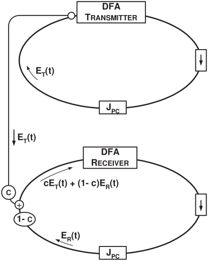
FIG. 1.: The setup of coupled DFRLs. The electric field circulating in the transmitter laser is $\mbox{{$\cal E$}}_{T}(t)$. After it is transmitted through a channel to the receiver, a fraction $c\mbox{{$\cal E$}}_{T}(t)$ is injected into the input of the rare earth doped amplifier in the receiver ring. At the same time a fraction $(1-c)\mbox{{$\cal E$}}_{R}(t)$ of the field circulating in the receiver ring is added to it, so the net field injected into the amplifier input is $c\mbox{{$\cal E$}}_{T}(t)+(1-c)\mbox{{$\cal E$}}_{R}(t)$.

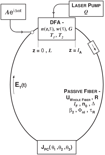
FIG. 2.: A schematic diagram showing the relevant location of the parameters we consider in our model of coupled rare-earth-doped fiber lasers.

FIG. 3.: Time to synchronization for identical DFRLs. The synchronization time $\tau_{s}$ is the time at which the amplitude synchronization error quantity $H_{E}(c,t)$ goes smaller than $\epsilon=10^{-2}$ and stays below for all larger times $t>\tau_{s}$. The value of $\tau_{s}$ is then averaged over 25 different initial conditions.

FIG. 4.: Amplitude synchronization error $D_{E}(c)$ for identical DFRLs. The DFRLs are first coupled for $20,000\tau_{R}$ and then the error term is averaged over an additional $3,000\tau_{R}$. The result is then averaged over 25 initial conditions.

FIG. 5.: Plot of $D_{E}(c)$ versus the number of round trips $N$ since coupling was initiated for coupling constants in the range of $0.01\leq c\leq 1.0$. The lasers are identical.

FIG. 6.: Plot of the rate of convergence for the measure $D_{E}(c)$ for a range of coupling constants. The slope is calculated beginning after the initial convergence upon coupling. The lasers are identical.

FIG. 7.: The dynamics of the integrated population inversion plotted against the number of round trips $N$ since coupling was initiated in the range $0.002\leq c\leq 0.2$. The lasers are identical.

FIG. 8.: Generalized synchronization measures $D_{I}(c)$, $D_{\phi}(c)$, and $D_{\theta}(c)$ plotted against coupling constant c. The DFRLs are coupled for $20,000\tau_{R}$ and the measures are taken over an additional $3,000\tau_{R}$. The lasers are identical.

FIG. 9.: Identical synchronization error $D_{E}(c)$ for DFRLs with gain mismatch $\cal{G}$. The DFRLs are first coupled for $20,000\tau_{R}$ and then the error term is calculated over an additional $3,000\tau_{R}$.

FIG. 10.: Generalized synchronization measures plotted against coupling constant c. There is gain mismatch. The filled symbols represent ${\cal{G}}=10\%$ and the clear symbols ${\cal{G}}=50\%$. The DFRLs are coupled for $20,000\tau_{R}$ and the measures are taken over an additional $3,000\tau_{R}$.

FIG. 11.: Identical synchronization error $D_{E}(c)$ for DFRLs with pump mismatch $\cal{Q}$. The DFRLs are first coupled for $20,000\tau_{R}$ and then the error term is calculated over an additional $3,000\tau_{R}$.

FIG. 12.: Generalized synchronization measures plotted against coupling constant c. There is pump mismatch. The filled symbols represent ${\cal{Q}}=10\%$ and the clear symbols ${\cal{Q}}=50\%$. The DFRLs are coupled for $20,000\tau_{R}$ and the measures are taken over an additional $3,000\tau_{R}$.

FIG. 13.: Identical synchronization error $D_{E}(c)$ for DFRLs with $\theta_{2}$ mismatch. There is nearly equal absorption, $R_{x}\approx R_{y}$. The DFRLs are first coupled for $20,000\tau_{R}$ and then the error term is averaged over an additional $3,000\tau_{R}$.

FIG. 14.: Generalized synchronization measures for DFRLs with $\theta_{2}$ mismatch. There is nearly equal absorption, $R_{x}\approx R_{y}$. The filled symbols represent a mismatch of $\theta_{2}=\pi/15$ and the clear symbols $\theta_{2}=\pi/3$. The DFRLs are first coupled for $20,000\tau_{R}$ round trips and then the error terms are averaged over an additional $3,000\tau_{R}$.

FIG. 15.: Identical synchronization error $D_{E}(c)$ for DFRLs with phase mismatch. The lasers are otherwise identical. The DFRLs are first coupled for $20,000\tau_{R}$ and then the error term is averaged over an additional $3,000\tau_{R}$.

FIG. 16.: Generalized synchronization measures plotted against coupling constant c. There is phase mismatch. The lasers are otherwise identical. The filled symbols represents $\tau_{\phi}=1\mu s$ and the clear symbols $\tau_{\phi}=10\mu s$. The DFRLs are coupled for $20,000\tau_{R}$ and the measures are taken over an additional $3,000\tau_{R}$.

FIG. 17.: Synchronization errors for DFRLs with a length mismatch of $\approx 80\mathrm{ps}$. The lasers are otherwise identical. The DFRLs are first coupled for $20,000\tau_{R}$ and then the error terms are averaged over an additional $3,000\tau_{R}$.

FIG. 18.: Synchronization errors for identical DFRLs with channel noise. The filled symbols represent SNR = 0 dB and the clear symbols SNR = 40 dB. The DFRLs are first coupled for $20,000\tau_{R}$ and then the error terms are averaged over an additional $3,000\tau_{R}$.

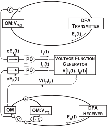
FIG. 19.: Diagram of optical modulation coupling scheme. All optical modulators (OM) are biased to a voltage of $V_{\pi/2}$. The optical fields of the transmitter and receiver are detected by photodiodes (PD) and fed into a voltage function generator. This voltage is then used to electro-optically modulate the $c$ branch of the receiver’s ring to bring the receiver DFRL into a state of generalized intensity synchronization with the transmitter DRFL’s intensity.

FIG. 20.: Synchronization errors for identical DFRLs with coupling by an optical modulator. The DFRLs are first coupled for $20,000\tau_{R}$ and then the error terms are averaged over an additional $3,000\tau_{R}$.

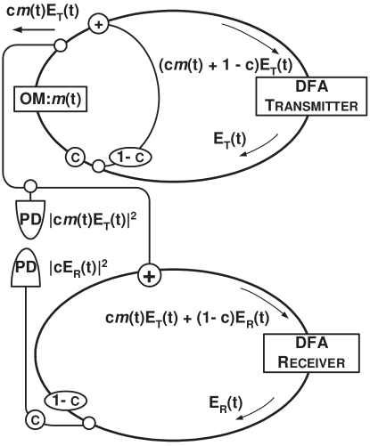
FIG. 21.: Diagram of communications using optical coupling scheme. The setup is almost identical to Fig. 1 except it contains and additional $c:1-c$ branch in the transmitter. This branch must be included if synchronization is to be achieved for couplings in the range $0<c<1$. Note for $\mbox{{$\cal E$}}_{T}(t)=\mbox{{$\cal E$}}_{R}(t)$, the optical fields entering both active mediums are identical, even with the presence of modulation.

FIG. 22.: Bit error rate versus coupling for the case of identical lasers using the two different coupling schemes. The coupling range is $0.0\leq c\leq 0.06$. The encoding is done via ASK modulation at a bit rate of 1 GHz with modulation factor $K=0.1$.

FIG. 23.: Bit error rate versus coupling for the case of optically coupled identical lasers in the presence of communication channel noise. The encoding is done via ASK modulation at a bit rate of 1 GHz with a modulation factor of $K=0.1$.

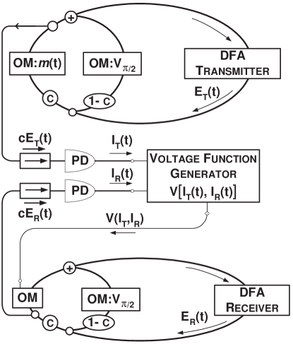
FIG. 24.: Diagram of communications using optical modulation coupling scheme. Again, the scheme is almost identical to Fig. 19 except for the presence of a $c:1-c$ branching in the transmitter. Again, this is added in an attempt to achieve synchronization in the presence of modulation for couplings in the range $0<c<1$.

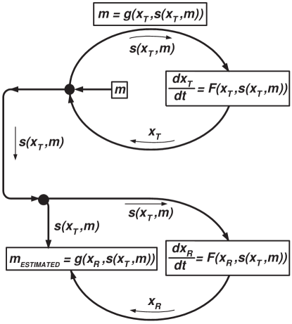
FIG. 25.: Cryptographic Setting of our $c=1$ communications scheme. This is known as a “Self-synchronous stream cipher in cipher feedback mode (CFB)”

TABLE I.: Typical parameters for the EDFRL model simulations

Quantity	Symbol	Value
Linear birefringence	$\Delta$	$1.8\times 10^{-6}$
Fiber index of refraction	$n_{0}$	$1.45$
External injection amplitude	$A$	0.0
Pump strength	$Q$	$2.4\times 10^{-2}$
Overall gain term	$G$	$1.35\times 10^{-2}$
Absorption coefficients	$R_{x}$, $R_{y}$	$0.45$, $0.449995$
Polarization controller angles	$\theta_{1}$, $\theta_{2}$, $\theta_{3}$	$0.5$, $1.2$, $1.5$
Nonlinear phase shift	$\Phi_{nl}$	$1.5\times 10^{-2}$
Round trip time	$\tau_{R}$	$200$ ns
Excited state lifetime	$T_{1}$	$10$ ms
Polarization dephasing time	$T_{2}$	$1$ ps
GVD coefficient	$\beta_{2}$	$-20\mathrm{ps}^{2}/\mathrm{km}$
Active fiber length	$l_{A}$	$20$ m
Passive fiber length	$l_{F}$	$20$ m

REFERENCES

- [1] Also: Department of Physics, UC San Diego. Electronic addresses: ctl@ucsd.edu (CTL). mbuhl@click.ucsd.edu (MB), lilling@ucsd.edu (LI).
- [2] Also: Department of Physics, and Marine Physical Laboratory, Scripps Institution of Oceanography, UC San Diego. Electronic address: hdia@jacobi.ucsd.edu
- [3] Electronic address: mkennel@ucsd.edu
- [4] H. D. I. Abarbanel, M. B. Kennel, M. Buhl, and C. T. Lewis, “Chaotic dynamics in erbium-doped fiber ring lasers”, to be published in Phys. Rev. A. (in press)
- [5] H. D. I. Abarbanel, and M. B. Kennel, Phys. Rev. Lett., 80 3153-3156 (1998).
- [6] R. Roy and G. VanWiggeren, Science, 279, 1198-1200 (1998).
- [7] G. VanWiggeren and R. Roy, Phys. Rev. Lett., 81, 3547-3550 (1999).
- [8] R. Roy. and G. VanWiggeren, private communication.
- [9] H. Fujisaka and T. Yamada, “Stability Theory of Synchronized motion in Coupled-Oscillator Systems”, Prog. Theor. Phys. 69, 32-47 (1983).
- [10] V.S. Afraimovich, N. N. Veirchev, and M. I. Rabinovich, “General Synchronization”, Izv. VUZ. Radiophiz. 29, 795-803 (1986).
- [11] D. Hansel, and H. Sompolinsky, “Synchronization and Computation in a Chaotic Neural Network”, Physical Review Letters 68, 718-721 (1991).
- [12] L. M. Pecora and T. L. Carroll, “Synchronization in Chaotic Systems”, Phys. Rev. Lett. 64, 821-824 (1990).
- [13] See the papers in the Special Issue of the IEEE Transactions on Circuits and Systems I: Fundamental Theory and Applications, Volume 44, Number 10, M. P. Kennedy and M. Ogorzalek, editors; October, 1997.
- [14] N. F. and A. Volkovskii, Tech. Phys. Lett., 19 97 (1993).
- [15] L. Kocarev and U. Parlitz, “General Approach for Chaotic Synchronization with Applications to Communication”, Physical Review Letters, 74 5028-5031 (1995).
- [16] M. M. Sushchik, N. F. Rulkov, L. Larson, L. Sh. Tsimring, H. D. I. Abarbanel, and K. Yao, “Chaotic Pulse Modulation: a Robust Method of Communicating with Chaos”, submitted to IEEE Communications Letters, January, 1999.
- [17] G. P. Agrawal, Nonlinear Fiber Optics, 2nd ed. (Academic Press, San Diego, 1995).
- [18] C. D. Poole, and R. E. Wagner, “Phenomenological Approach to Polarisation Dispersion in Long Single-Mode Fibers”, Electronics Letters 22, 1029-1030 (1986).
- [19] R. Brown and L. Kocarev, “A Unifying Definition of Synchronization for Dynamical Systems”, Los Alamos preprint, (1999).
- [20] N. F. Rulkov, M. M. Sushchik, L. S. Tsimring, and H. D. I. Abarbanel, “Generalized Synchronization of Chaos in Directionally Coupled Chaotic Systems”, Phys. Rev. E 51 980-994 (1995).
- [21] L. Kocarev and U. Parlitz, “Generalized Synchronization, Predictability, and Equivalence of Unidirectionally Coupled Dynamical Systems.” Phys. Rev. Lett. 76,1816 (1996).
- [22] U. Parlitz, L. Junge, and L. Kocarev, “Subharmonic Entrainment of Unstable Periodic Orbits and Generalized Synchronization.” Phys. Rev. Lett. 79, 3158-61 (1997).
- [23] B. R. Hunt, E. Ott, and J. A. Yorke, “Differentiable Generalized Synchronization.” Phys. Rev. E 55, 4029 (1997).
- [24] R. Brown, “Approximating the Mapping Between Systems Exhibiting Generalized Synchronization.” Phys. Rev. Lett 81, 4835 (1998).
- [25] N. F. Rulkov, and M. M. Sushchik, Phys. Lett. 214A, 145 (1996).
- [26] S. Betti, G. DeMarchis, and E. Iannone, Coherent Optical Communications Systems Wiley (1995).
- [27] H. D. I. Abarbanel, M. B. Kennel, M. Buhl, L. Illing, and C. T. Lewis, “Synchronization of Optical Ring Lasers by Electro-Optic Modulation.”, in preparation, (1999).
- [28] A. Yariv,Optical Electronics CBS College (1985).
- [29] S. H. Chuang,Physics of Optoelectric Devices Wiley (1995).
- [30] D. Denning,Cryptography and Data Security Addison-Wesley (1982).
- [31] G. J. Kühn, “Algorithms for Self-Synchronizing Ciphers”, Proceedings of Comsig’88, Southern African Conference on Communications and Signal Processing, Pretoria, 24 June 1988.
- [32] H. M. Heys and S. E. Tavares, “Cryptanalysis of Tree-Structured Substitution-Permutation Networks”, Electronics Letters 29, 40-41 (1993).
- [33] R. J. Anderson, “Faster Attack on Certain Stream Ciphers”, Electronic Letters 29, 1322-1323 (1993).
- [34] W. Millan, E. P. Dawson, and L. J. O’Conner, “Cryptanalysis of Tree-structured Ciphers”, Electronic Letters 30, 941-942 (1994).
- [35] T. Siegenthaler, “Decrypting a Class of Stream Ciphers Using Ciphertext Only”, IEEE Transactions on Computers C-34, 81-85 (1985).
- [36] R. A. Rueppel, “Stream Ciphers”, Contemporary Cryptology: The Science of Information Integrity, IEEE Press, New York, (1991), ed. G. Simmons, pp. 65-134.
- [37] H. D. I. Abarbanel, M. B. Kennel, L. Illing, C. T. Lewis, and M. Buhl, “Synchronization and Communication in Chaotic Semiconductor Lasers”, to be submitted to Physical Review E.