Learning Driver-Response Relationships from Synchronization Patterns

We test recent claims that causal (driver/response) relationships can be deduced from interdependencies between simultaneously measured time series. We apply two recently proposed interdependence measures which should give similar results as cross predictabilities used by previous authors. The systems which we study are asymmetrically coupled simple models (Lorenz, Roessler, and Henon models), the couplings being such as to lead to generalized synchronization. If the data were perfect (noisefree, infinitely long), we should be able to detect, at least in some cases, which of the coupled systems is the driver and which the response. This might no longer be true if the time series has finite length. Instead, estimated interdependencies depend strongly on which of the systems has a higher effective dimension at the typical neighborhood sizes used to estimate them, and causal relationships are more difficult to detect. We also show that slightly different variants of the interdependence measure can have quite different sensitivities.

1 Introduction

The study of synchronization between chaotic systems has been a topic of increasing interest since the beginnings of the ’90s. One important step in this direction was the introduction of the concept of generalized synchronization [1, 2, 3], extending previous studies of coupled identical systems (identical synchronization [4, 5, 6, 7, 8, 9]) to the study of coupled systems with different dynamics.

Let us denote by ${\bf X}$ and ${\bf Y}$ two dynamical systems, and by ${\bf x}=\{x_{1},\ldots,x_{d}\}$ and ${\bf y}=\{y_{1},\ldots,y_{r}\}$ their state vectors, obtained for example by delay embedding. We assume in the following that the dynamics is deterministic with continuous time (the case of maps is completely analogous, and will be treated in Secs. 3 and 4). We further assume the systems are unidirectionally coupled, say ${\bf X}$ is the autonomous driver and ${\bf Y}$ the driven response

$$\dot{{\bf x}}(t) = F({\bf x}(t))\;,$$

$$\dot{{\bf y}}(t) = G({\bf y}(t),{\bf x}(t))$$ (1)

We speak about generalized synchronization between ${\bf X}$ and ${\bf Y}$ if the following relation exists:

$${\bf y}(t)=\Psi({\bf x}(t))$$ (2)

This requirement is less restrictive than the one of identical synchronization, in which $\Psi=1$. Equation (2) implies that the state of the response system is a function only of the state of the driver. It is not to be confused with the opposite relation ${\bf x}(t)=\Phi({\bf y}(t))$ (considered in [10]), which is generically valid for sufficiently high embedding dimensions if the coupling is non-singular, in the sense of obeying $\det(\partial G_{i}/\partial x_{n})\neq 0$ everywhere. This follows from the implicit function theorem, which allows us to invert eq.(1b) to ${\bf x}=\chi({\bf y},\dot{{\bf y}})$, and from the fact that $\tilde{\bf y}(t)=({\bf y}(t),\dot{\bf y}(t))$ is as good a state vector as ${\bf y(t)}$. In particular, if we consider $G({\bf y}(t),{\bf x}(t))=H({\bf y}(t))+U({\bf x}(t))$, we immediately have ${\bf x}(t)=U^{-1}(\dot{{\bf y}}(t)-H({\bf y}(t)))$ if $U({\bf x})$ can be inverted.

The transformation $\Psi$ does not need to be smooth as considered in [3, 11] and explicitly required in [12, 13]. In fact, Pyragas [14] defined as strong and week synchronizations the cases of smooth and non-smooth transformations, respectively (see also [15]).

If one of the systems drives the other and a relationship like equation (2) exists, it is possible to predict the response from the simultaneous state of the driver. But the opposite is not true. Just knowing that a relationship like equation (2) exists and that the state of ${\bf Y}$ can be predicted from that of ${\bf X}$, it is in general not possible to establish which is the driver and which is the response. This is obvious when $\Psi$ is bijective (i.e., $\Phi=\Psi^{-1}$ exists and is unique). The above arguments tell us that $\Psi$ is indeed likely to be bijective in case of generalized synchronization, at least for nearly all ${\bf x}$: If a coupling is not regular in the above sense, then its singularities are typically located on a set of measure zero. One might tend to believe that ${\bf X}$ must control ${\bf Y}$ (and not the opposite), if ${\bf y}$ follows the motion of ${\bf x}$ with a positive time delay. But even then one cannot be sure since there could be an internal delay loop in ${\bf Y}$ which causes the emitted time series to lag behind. Also, both systems could be driven by a third system. Thus, detecting causal relationships is not easy in general, although it is of course of utmost importance in many applications.

In the above we pretended that we could detect exactly whether the state of one of the systems is a function of the other. This is of course never the case in practical applications. Different observables which should enable one to detect interdependencies in realistic cases were introduced by several authors. Following an original idea of Rulkov et al. [3, 11], mutual cross-predictabilities were defined and studied by Schiff et al. [17] and Le van Quyen et al. [16, 10]. A quantity more closely related to that of [3], but optimized for robustness to noise and imperfections in the data was used in [18]. In the latter paper also a number of other variants were discussed. Some of these variants were tested and found to be inferior, but no systematic tests were made.

In contrast to our above discussion, the authors of [17] and [16, 10] claimed that driver/response relationships can be deduced from such interdependencies. But their proposals, backed by numerical studies of simple model systems, were mutually contradictory. While it was argued in [17] that the driver state ${\bf x}$ should be more dependent on the response state ${\bf y}$ (i.e., there exists a stronger functional dependency ${\bf y}\stackrel{{\scriptstyle\Phi}}{{\to}}{\bf x}$) than vice versa (which is, as we said, a bit counter intuitive), exactly the opposite was claimed in [16, 10]. Finally, in [18] it was claimed that neither can be expected to be correct in realistic situations with finite noisy data, and that it is in general the system with more excited degrees of freedom (the more ‘active’ system) that is more independent, while the state of the more ‘passive’ system (with less excited degrees of freedom) depends on it.

It is the purpose of the present work to settle this question by carefully studying simple toy models, including Lorenz, Roessler, and Henon systems, using two of the interdependence measures proposed in [18]. Basic notions involved in generalized synchronization are reviewed in Sec.2. In Sec.3, we recall the operational definition of interdependence used in [18]. Numerical results are presented in Sec.4, and our conclusion is drawn in Sec.5.

2 Generalized Synchronization with Exactly Known Dynamics

While identical synchronization is easily visualized by plotting the difference between one of the coordinates of the driver and the corresponding coordinate of the response, no similarly simple way exists to detect generalized synchronization. Constructing the function $\Psi$ explicitly [19] might be possible in particularly simple cases, but since this will be never exact, it will be never clear whether deviations from eq.(2) are due to lack of synchronization or inexactness of $\Psi$. Instead, the methods of choice in cases where the exact equations of motion are known and where arbitrary initial states can be prepared are the study of Lyapunov exponents and the identical synchronization of two identical response systems differing in their initial conditions.

For the driver/response systems as in eq.(1), one has $d+r$ different Lyapunov exponents. Of these, $d$ exponents coincide with those of the (autonomous) driver denoted by $\lambda^{({\bf X})}_{i},\;i=1\ldots d$. The other $r$ exponents coincide with those of the response, considered as a non-autonomous system driven by the external signal ${\bf x}(t)$ (called conditional Lyapunov exponents in [8]) . They will be called $\lambda^{({\bf Y})}_{i},\;i=1\ldots r$. Ranking the Lyapunov exponents as usual by magnitude, we have generalized synchronization iff $\lambda^{({\bf Y})}_{1}<0$.

Furthermore, once the Lyapunov exponents are known, the dimension of the combined system ${\bf X}+{\bf Y}$ can be estimated from the Kaplan-Yorke formula [20]

$$D_{{\bf X}+{\bf Y}}=l+\sum_{j=1}^{l}\frac{\lambda_{j}}{|\lambda_{l+1}|}$$ (3)

(here, $l$ is the largest integer for which the sum over $j$ is non negative). Generically, we must expect this also to be the dimension of ${\bf Y}$ alone . The reason is that, as pointed out in the introduction, ${\bf X}$ will be a (single- or multivalued) function of ${\bf Y}$, if the inverse of $G({\bf x},{\bf y})$ is single- or multivalued. On the other hand, the Kaplan-Yorke dimension of ${\bf X}$ alone may be equal to $D_{{\bf X}+{\bf Y}}$ or smaller. It is given by a formula similar to eq.(3) but with $\lambda_{i}$ replaced by $\lambda^{({\bf X})}_{i}$. We see that

$$D_{{\bf X}}<D_{{\bf X}+{\bf Y}}\qquad{\rm iff}\qquad\lambda_{1}^{({\bf Y})}>\lambda_{l+1}^{({\bf X})},$$ (4)

where $l$ is determined by $\sum_{j\leq l}\lambda_{j}^{({\bf X})}\leq 0<\sum_{j\leq l+1}\lambda_{j}^{({\bf X})}$. If this inequality holds (together with $\lambda_{1}^{({\bf Y})}<0$), we have weak synchronization in the sense of Pyragas [14]. In the opposite case, i.e. $\lambda_{1}^{({\bf Y})}\leq\lambda_{l+1}^{({\bf X})}$, one is likely to have strong synchronization, although this might not be true due to multifractality: Due to the latter, it is possible that the box-counting dimension of ${\bf X}$ is strictly smaller than that of ${\bf X}+{\bf Y}$, although the equality holds for the Kaplan-Yorke (i.e., information) dimensions. In such a case $\Psi$ cannot be smooth, but regions where $\Psi$ is non-smooth might well be of measure zero [15].

Another approach for detecting generalized synchronization is by using two identical response systems which differ only in their initial conditions. If these replicas get synchronized after some transient, their trajectories are obviously independent of the initial conditions, thus being only a function of the driver. This is most easily checked visually, e.g. by plotting the difference between two analogous components of the two replicas against time. In this way one can also check for intermittencies and long transients which can, together with finite numerical resolution, severely obscure the interpretation.

3 Generalized Synchronization in Real Life

The above considerations depend on the availability of the exact equations of motion, and on the ability to prepare identical replicas. Neither holds for typical applications.

Real signals usually consist of short segments of data contaminated by noise. Furthermore, the dynamics of the system is not known, and therefore the methods described in the previous section are not applicable.

While identically synchronized systems describe the same trajectory in the phase space, the hallmark of a relationship as in eq.(2) is that any recurrence of ${\bf X}$ implies a recurrence of ${\bf Y}$. If ${\bf X}$ comes exactly back to a state it had already been in before, the same must be true for ${\bf Y}$. In real data, one cannot of course expect exact recurrence. We will therefore use as a criterion that whenever two states of ${\bf X}$ are similar, the contemporary states of ${\bf Y}$ are also similar.

In [17, 16, 10], this was implemented by making forecasts of ${\bf x}_{n}$ using local neighborhoods (e.g., by means of locally linear maps), and comparing the quality of these forecasts with that of forecasts based on “wrong” neighborhoods. In the latter, the nearest neighbors of ${\bf x}_{n}$ are replaced by the equal time partners of the nearest neighbors of ${\bf y}_{n}$. For reasons explained in [18], we prefer to use instead a measure closer to the original proposal of Rulkov et al. [3]. But we should stress that we see no reason why our results should not be carried over to the observables used in [17, 16, 10] immediately.

Let us suppose we have two simultaneously measured univariate time series from which we can reconstruct $m$-dimensional delay vectors [21] ${\bf x}_{n}=(x_{n},\ldots,x_{n-m+1})$ and ${\bf y}_{n}=(y_{n},\ldots,y_{n-m+1})$, $n=1,\ldots N$.

Let $r_{n,j}$ and $s_{n,j}$, $j=1,\ldots,k$, denote the time indices of the $k$ nearest neighbors of ${\bf x}_{n}$ and ${\bf y}_{n}$, respectively. For each ${\bf x}_{n}$, the squared mean Euclidean distance to its $k$ neighbors is defined as

$$R_{n}^{(k)}({\bf X})=\frac{1}{k}\sum_{j=1}^{k}{\left({\bf x}_{n}-{\bf x}_{r_{n,j}}\right)^{2}}$$ (5)

and the Y-conditioned squared mean Euclidean distance is defined by replacing the nearest neighbors by the equal time partners of the closest neighbors of ${\bf y}_{n}$,

$$R_{n}^{(k)}({\bf X}|{\bf Y})=\frac{1}{k}\sum_{j=1}^{k}{\left({\bf x}_{n}-{\bf x}_{s_{n,j}}\right)^{2}}.$$ (6)

If the point cloud $\{{\bf x}_{n}\}$ has average squared radius $R({\bf X})=\langle R^{(N-1)}({\bf X})\rangle$ and effective dimension $D$ (for a stochastic time series embedded in $m$ dimensions, $D=m$), then $R_{n}^{(k)}({\bf X})\ll R({\bf X})$ for $k\ll N$. More precisely, we expect

$$R_{n}^{(k)}({\bf X})/R({\bf X})\sim(k/N)^{2/D},$$ (7)

where $D$ is the dimension of the probability measure from which the points ${\bf x}_{n}$ are drawn. Furthermore, $R_{n}^{(k)}({\bf X}|{\bf Y})\approx R_{n}^{(k)}({\bf X})\ll R({\bf X})$ if the systems are strongly correlated, while $R_{n}^{(k)}({\bf X}|{\bf Y})\gg R_{n}^{(k)}({\bf X})$ if they are independent. Accordingly, we can define an interdependence measure $S^{(k)}({\bf X}|{\bf Y})$ as

$$S^{(k)}({\bf X}|{\bf Y})=\frac{1}{N}\sum_{n=1}^{N}\frac{R_{n}^{(k)}({\bf X})}{R_{n}^{(k)}({\bf X}|{\bf Y})}.$$ (8)

Since $R_{n}^{(k)}({\bf X}|{\bf Y})\geq R_{n}^{(k)}({\bf X})$ by construction, we have

$$0<S^{(k)}({\bf X}|{\bf Y})\leq 1.$$ (9)

Low values of $S^{(k)}({\bf X}|{\bf Y})$ indicate independence between ${\bf X}$ and ${\bf Y}$, while high values indicate synchronization (becoming maximal when $S^{(k)}({\bf X}|{\bf Y})\to 1$).

The opposite interdependence $S^{(k)}({\bf Y}|{\bf X})$ is defined in complete analogy. It is in general not equal to $S^{(k)}({\bf X}|{\bf Y})$. If $S^{(k)}({\bf X}|{\bf Y})>S^{(k)}({\bf Y}|{\bf X})$, i.e. if ${\bf X}$ depends more on ${\bf Y}$ than vice versa, instead of assuming a causal relationship, we just say that ${\bf Y}$ is more “active” than ${\bf X}$. As was argued in [18], high activity is mainly due to a large effective dimension $D$, on the typical length scale set by the distances $|{\bf x}_{n}-{\bf x}_{r_{n,k}}|$ and $|{\bf x}_{n}-{\bf x}_{s_{n,k}}|$.

The second interdependence measure to be used in this work was also introduced in [18]. In eq.(8) we essentially compare the ${\bf Y}$-conditioned mean squared distances to the unconditioned m.s. nearest neighbor distances. Instead of this, we could have compared the former to the m.s. distances to random points, $R_{n}({\bf X})=(N-1)^{-1}\sum_{j\neq n}({\bf x}_{n}-{\bf x}_{j})^{2}$. Also, in ergodic theory often geometric averages are more robust and more easy to interpret than arithmetic ones. Therefore, let us use the geometrical average in the analogon of eq.(8), and define

$$H^{(k)}({\bf X}|{\bf Y})=\frac{1}{N}\sum_{n=1}^{N}\log\frac{R_{n}({\bf X})}{R_{n}^{(k)}({\bf X}|{\bf Y})}$$ (10)

This is zero if ${\bf X}$ and ${\bf Y}$ are completely independent, while it is positive if nearness in ${\bf Y}$ implies also nearness in ${\bf X}$ for equal time partners. It would be negative if close pairs in ${\bf Y}$ would correspond mainly to distant pairs in ${\bf X}$. This is very unlikely but not impossible. Therefore, $H^{(k)}({\bf X}|{\bf Y})=0$ suggests that ${\bf X}$ and ${\bf Y}$ are independent, but does not prove it. This (and the asymmetry under the exchange ${\bf X}\leftrightarrow{\bf Y}$) is the main difference between $H^{(k)}({\bf X}|{\bf Y})$ and mutual information. The latter is strictly positive whenever ${\bf X}$ and ${\bf Y}$ are not completely independent. As a consequence, mutual information is quadratic in the correlation $P({\bf X},{\bf Y})-P({\bf X})P({\bf Y})$ for weak correlations ($P$ are here probability distributions), while $H^{(k)}({\bf X}|{\bf Y})$ is linear. Thus $H^{(k)}({\bf X}|{\bf Y})$ is more sensitive to weak dependencies which might make it useful in applications. Also, it should be easier to estimate than mutual informations which are notoriously hard to estimate reliably.

4 Numerical Examples

The aim of this section is to see numerically whether there exists any relationship between the ‘activity’ defined in the last section, and a driver/response relationship. In principle there should exist such a relationship, since we have argued that the system with higher dimension should be more active, and usually the response does have higher dimension. This would agree with the conclusion of [17], and contradict [16, 10]. But it is well known that observed attractor dimensions can be quite different from real ones, in particular if one has only a finite amount of noisy data and weakly coupled systems [22].

In order to obtain results which can be easily compared to those of [17, 16, 10], we study the same systems as these authors.

4.1 Lorenz Driven by Rössler

As a first example, we studied the unidirectionally coupled systems proposed in reference [10]. The driver is an autonomous Rössler system with equations:

$$\dot{x}_{1} = -\alpha\{x_{2}+x_{3}\}$$

$$\dot{x}_{2} = \alpha\{x_{1}+0.2\;x_{2}\}$$ (11)

$$\dot{x}_{3} = \alpha\{0.2+x_{3}(x_{1}-5.7)\}$$

which drives a Lorenz system in which the equation for $\dot{y}_{2}$ is augmented by a driving term involving $x_{2}$,

$$\dot{y}_{1} = 10(-y_{1}+y_{2})$$

$$\dot{y}_{2} = 28\;y_{1}-y_{2}-y_{1}\;y_{3}+C\;x_{2}^{2}$$ (12)

$$\dot{y}_{3} = y_{1}\;y_{2}-\frac{8}{3}y_{3}.$$

The unidirectional coupling is introduced in the last term of the second equation, the constant $C$ being its strength. Notice that $x_{2}$ enters quadratically in the coupling, whence it cannot be written as a univalent function of $y_{1},y_{2},y_{3}$, and $\dot{y}_{2}$. Thus we do not have a strict argument telling us that $D_{{\bf Y}}\geq D_{{\bf X}}$, but the latter seems extremely likely.

As in reference [10] the parameter $\alpha$ is introduced in order to control the relative frequencies between the two systems. The differential equations were iterated, together with the equations for the tangent vectors, by using fourth and fifth order Runge-Kutta algorithms with $\Delta t=0.003-0.009$. This was checked to yield numerically stable results, while larger $\Delta t$ and/or a third order algorithm would have given different results. In order to eliminate transients, the first $10^{6}$ iterations were discarded. From the increase of the tangent vectors during the following $10^{6}$ iterations we obtained the Lyapunov exponents. Delay vectors with delay $\tau=0.3$ and embedding dimensions 4 and 5 were constructed from $x_{1}(t)$ and $y_{1}(t)$. This delay corresponds to roughly 1/4 of the average period of the Lorenz equations. All time sequences had length $N=5000$. In order to check for stability and for very long transients, all computations were repeated several times with different initial conditions.

For the parameters considered here, the Lyapunov exponents of the Rössler are $\lambda_{i}\approx 0.09\alpha,\;0,\;-5\alpha$; and the ones of the Lorenz without coupling are $\lambda_{i}\approx 0.84,\;0,\;-14.5$. Figure 1 shows the maximum Lyapunov exponent of the driven Lorenz system, as a function of the coupling strength $C$. The continuous curve shows the result for $\alpha=6$, the broken one corresponds to $\alpha=10$. For generalized synchronization, the maximum Lyapunov exponent should be negative. When $\alpha=10$, this is observed for $2.1<C<2.7$ and for $c>2.9$. For all values of $C$ considered in fig. 1, the maximal Lyapunov exponent of the driven system is larger than the smallest one of the driver, and therefore we have only weak synchronization.

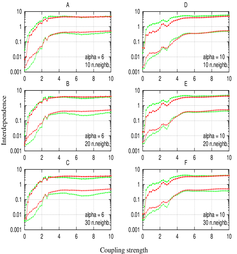
Figure 2: Non-linear interdependences between a Lorenz system driven by a Rössler system, plotted as a function of the coupling strength. Left side graphs correspond to $\alpha=6$ and right side graphs to $\alpha=10$. From top to bottom, the graphs are for 10, 20, and 30 nearest neighbors. $S({\bf Y}|{\bf X})$: black lines with crosses, $S({\bf X}|{\bf Y})$: grey lines with crosses, $H({\bf Y}|{\bf X})$: black lines with squares and $H({\bf X}|{\bf Y})$: grey lines with squares. See text for details.

Figure 2 shows the interdependencies $S({\bf X}|{\bf Y})$, $S({\bf Y}|{\bf X})$, $H({\bf X}|{\bf Y})$ and $H({\bf Y}|{\bf X})$ for $\alpha=6$ and $\alpha=10$, and for different number of nearest neighbors. The embedding dimension was $m=5$. In all panels, lines with crosses (lower curves) are for $S$ and lines with squares (upper curves) are for $H$; the dark lines denote $({\bf Y}|{\bf X})$ interdependencies and the grey lines are for $({\bf X}|{\bf Y})$. All interdependencies rise with the coupling strength, with only few exceptions. These exceptions (at $C\approx 2.5$ for $\alpha=6$ and at $2.3<C<2.8$ for $\alpha=10$) occur exactly at places where the maximal Lyapunov exponent of the driven system is non-monotonic. Thus the dependencies are monotonic functions of the Lyapunov exponent. The measure $S$ is more sensitive to the sign of the Lyapunov exponent than is $H$, as seen from the sharper increase of $S$ when the Lyapunov exponent passes through zero and the systems synchronize.

In reference [10] this system was studied only for $\alpha=6$ and $C=8$. The latter corresponds to very strong coupling. It was found that the interdependence of ${\bf Y}$ from ${\bf X}$ was larger than vice versa. This was taken as a proof that in general the response depends more on the driver than vice versa, and it was proposed that this result could be used as a general method to detect driver/response relations.

Our results with $S$ and $H$ agree perfectly with those of [10], if we keep the same values for $\alpha$ and $C$, and use $k\geq 20$, i.e. for large neighborhoods. In case of $S$ we find $S({\bf Y}|{\bf X})\geq S({\bf X}|{\bf Y})$ for all $k$ and $\alpha$, provided $C>5$. Finally, we also find the same inequality $S({\bf Y}|{\bf X})>S({\bf X}|{\bf Y})$ for very small couplings (below the synchronization threshold), while the opposite inequality sometimes holds for intermediate $C$.

A more consistent picture is seen in the behavior of $H({\bf X}|{\bf Y})$ and $H({\bf Y}|{\bf X})$. Except in the case $\alpha=6,C>4$, and $k\geq 20$, we always found $H({\bf X}|{\bf Y})>H({\bf Y}|{\bf X})$, in agreement with the prediction of [17]. This inequality is most pronounced for small values of $C$.

Our results can be understood by the following heuristic arguments:

• For strong couplings the two systems are so strongly synchronized that the differences in interdependence are small, and we can predict ${\bf X}$ from ${\bf Y}$ essentially as well as ${\bf Y}$ from ${\bf X}$.

• The theoretical predictions $H({\bf X}|{\bf Y})>H({\bf Y}|{\bf X})$ and $S({\bf X}|{\bf Y})>S({\bf Y}|{\bf X})$ are based on the limiting behavior for small neighborhoods. It is thus not too surprising that they can be violated for large values of $k$.

• For uncoupled systems ($C=0$) one has $S({\bf X}|{\bf Y})<S({\bf Y}|{\bf X})$ if $D_{\bf X}<D_{{\bf Y}}$ and vice versa. Notice that this (which is easily obtained from eq.(7)) is the opposite of what we expect if $D_{\bf X}<D_{{\bf Y}}$ holds only due to the coupling. In our case, $D_{\rm Roessler}\approx 2.018<D_{\rm Lorenz}\approx 2.058$. This explains why $S({\bf X}|{\bf Y})<S({\bf Y}|{\bf X})$ for very small $C$ ($C<1$). In contrast, $H({\bf X}|{\bf Y})=H({\bf Y}|{\bf X})=0$ for uncoupled systems, whence no such problem exists for $H$. Thus we expect that the behavior of $H({\bf X}|{\bf Y})$ at small couplings is easier to interpret than the behavior of $S$ which should depend nontrivially on $k$ and $N$. This is precisely what we found.

4.2 Two Coupled Henon Maps

As a second example we studied two unidirectionally coupled Henon maps similar to the ones proposed in [17], with equations

$$x^{\prime}_{1} = 1.4-x_{1}^{2}+b_{1}\;x_{2}$$

$$x^{\prime}_{2} = x_{1}$$ (13)

for the driver, and

$$y^{\prime}_{1} = 1.4-(C\;x_{1}y_{1}+(1-C)\;y_{1}^{2})+b_{2}\;y_{2}$$

$$y^{\prime}_{2} = y_{1}$$ (14)

for the response. Again we discarded the first $10^{6}$ iterations, and obtained Lyapunov exponents from the next $10^{6}$. Interdependencies were then estimated from $N=5000$ iterations, using 3-dimensional delay vectors. As in the previous example, the stability of the results was checked by starting from different initial conditions. For calculating the interdependencies we used $k=10$ nearest neighbors. No significant changes were observed for other values of $k$.

The constants $b_{1}$ and $b_{2}$ were both set to 0.3 when analyzing identical systems, and to 0.3, 0.1 when analyzing non-identical ones. Furthermore, in all cases we also studied how the results changed if white measurement noise was added either to the driver, to the response, or to both.

4.2.1 Identical systems

We first studied the case $b_{1}=b_{2}=0.3$. This is the “canonical” value for the Henon map, for which $\lambda_{1}=0.4192$ and $D=1.26$. One easily sees that $(y_{1},y_{2})=(x_{1},x_{2})$ is a solution of eqs.(13,14). Thus we can have identical synchronization [8], but due to the asymmetry of the coupling we cannot rule out non-identical (generalized) synchronization either.

Figure 3 (solid line) shows the maximum Lyapunov exponent of the response system. It becomes negative for couplings larger than 0.7, when identical synchronization between the systems takes place. But it is also slightly negative for $0.47<C<0.52$. Plotting differences $x_{1}-y_{1}$, e.g., one sees that there is no identical synchronization in this window. But making a cut through the attractor of the combined system, by plotting e.g. pairs $(x_{2},y_{2})$ whenever $|x_{1}|<10^{-4}$, one sees a fractal structure which clearly shows that there is no identical synchronization. On the other hand, $\lambda_{1}^{({\bf Y})}<0$ which leaves only the possibility of generalized synchronization. In this window $(0.47<C<0.52)$, the Kaplan-Yorke formula gives $D\approx 2.25$, showing that this synchronization is weak. For $C>0.7$, the Kaplan-Yorke formula does of course not apply to the combined system and $D=D_{\rm Henon}=1.26$.

Interdependencies are shown in fig. 4A and fig. 4D. As expected, we see that $S$ and $H$ both rise sharply at $C\geq 0.7$, where identical synchronization sets in. The fact that synchronization is perfect is seen from the fact that $S({\bf Y}|{\bf X})=1$ for $C\geq 0.7$. In contrast, we do not see any anomaly for $C\approx 0.5$, showing again that the synchronization at $c\approx 0.5$ is very weak indeed. For $C<0.7$ we see that $H({\bf X}|{\bf Y})>H({\bf Y}|{\bf X})$, in agreement with our general prejudice that the response has higher dimension and is thus more active. Although not so pronounced, this difference is also seen for $S$.

We also analyzed how both measures changed with the inclusion of measurement noise ($S/N$ amplitude ratio $\sim 25\%$). Figs. 4B and 4E show the results when the noise is added to the driver and figs.4C and 4F when it is added to the response. In general, we expect of course a decrease of any dependences when noise is added. Formally, we have to discuss how $R^{(k)}({\bf X}|{\bf Y})$, $R^{(k)}({\bf Y}|{\bf X})$, $R^{(k)}({\bf X})$, and $R({\bf X})$ change if noise is added to ${\bf X}$.

• $R({\bf X})$ changes very little, since $S/N\ll 1$;

• $R^{(k)}({\bf X})$ increases strongly, since the dimension of the noisy time series is large;

• $R^{(k)}({\bf X}|{\bf Y})$ increases little if ${\bf X}$ and ${\bf Y}$ are weakly dependent (it is already large), but increases even more than $R^{(k)}({\bf X})$ if ${\bf X}$ and ${\bf Y}$ are strongly dependent.

• The last is also true for $R^{(k)}({\bf Y}|{\bf X})$.

From these we see that $H({\bf Y}|{\bf X})$ should decrease roughly as much as $H({\bf X}|{\bf Y})$, and this decrease should be strongest if ${\bf X}$ and ${\bf Y}$ are fully synchronized. In contrast, $S({\bf X}|{\bf Y})$ should decrease much less (or even increase) if noise is added to ${\bf X}$, and if ${\bf X}$ and ${\bf Y}$ are weakly dependent. If ${\bf X}$ and ${\bf Y}$ are fully synchronized, adding noise to ${\bf X}$ suppresses $S({\bf Y}|{\bf X})$ much more than $S({\bf X}|{\bf Y})$ since the strong increase of $R^{(k)}({\bf Y}|{\bf X})$ is then not compensated by any change of $R({\bf Y})$. Adding noise to ${\bf Y}$ can be discussed similarly. All these predictions are fully verified in fig.4. Notice that measurement noise can reverse the general inequality $H({\rm driver}|{\rm response})>H({\rm response}|{\rm driver})$, as seen e.g. in fig.4E for $C>0.7$.

In general, $S$ seems to be less robust against measurement noise than $H$.

4.2.2 Non identical systems

Figures 5A and 5D show dependencies for different $b$-parameters ($b_{1}=0.3,b_{2}=0.1$) where identical synchronization is impossible, and where the driver has higher dimension than the uncoupled response. In this case, the interdependencies do not increase as sharply as in the previous case, and they reach lower values. With both measures we see an increase between $C=0.1-0.4$ in agreement with the negative values of the maximum Lyapunov exponent for these coupling strengths (see fig.3). As in reference [17], we found $S({\bf X}|{\bf Y})>S({\bf Y}|{\bf X})$ and $H({\bf X}|{\bf Y})>H({\bf Y}|{\bf X})$. These inequalities still hold when adding measurement noise to the driver (fig.5B,E). But when the noise is added to the response (fig.5C,F), only the inequality for $H$ survives, while that for $S$ is reversed. These dependences on noise can be discussed in complete analogy with the previous case of identical systems.

The situation changes slightly if the uncoupled response has higher dimension than the driver, as in the case $b_{1}=0.1,b_{2}=0.3$ shown in fig. 6. The panels of this figure show more structure than those of fig.5, mainly since also the Lyapunov exponent shows more structure (see fig.3). From fig. 6F we see that there is a parameter window, $0.4\leq C\leq 0.6$, where $H({\bf Y}|{\bf X})>H({\bf X}|{\bf Y})$ after adding noise to ${\bf Y}$. This is not yet understood, but all other features in this plot can be understood heuristically along the lines discussed above.

5 Conclusion

In this work we studied the possibility of predicting driver/response relationships from asymmetries in nonlinear interdependence measures. More precisely, we studied two particular interdependence measures, introduced in [18], and applied them to simple asymmetrically coupled strange attractors. In contrast to previous works, we find that such predictions are not always reliable, although we agree with [17] that they would be possible for ideal (noise-free, infinitely long) data. We agree with [16, 10] as far as one of their numerical examples is concerned, but we show that this was a mere coincidence, and cannot be generalized.

Instead, we confirmed the conjecture of [18] that asymmetries in interdependence measures reflect mainly the different degrees of complexity of the two systems at the level of resolution at which these measures are most sensitive. For practical applications, this is not the infinitely fine level at which theoretical arguments like those of [17] apply. The latter predict correctly that the response is more complex, i.e. has a higher Kaplan-Yorke dimension. But this argument can become irrelevant even for the extremely simple toy models which we studied in the present paper. It should be even less relevant in realistic situations where all sorts of noise, non-stationarity, and shortness of data present additional limitations.

Nevertheless, we propose that asymmetries of measured interdependencies can be very useful in understanding coupled systems. Indications for this were given in [17, 16, 10, 18]. All these papers were dealing with neurophysiology. Even if no causal relationships can be deduced from such asymmetries, it was found in [16, 10, 18] that the resulting patterns are closely related to clinical observations, and could e.g. contribute to a more precise localization of epileptic foci and might be useful for predicting epileptic seizures.

An unexpected result of our study is that for the simulations performed the measure $H({\bf X}|{\bf Y})$ which had not done very well in preliminary tests is actually more robust and easier to interpret than the measure $S({\bf X}|{\bf Y})$ which was mostly used in [18]. However, this should not be directly extended to real life data. A more systematic comparative study with a large database of EEGs from epilepsy patients is under way.

Figure 1: Maximum Lyapunov exponents of the modified Lorenz system driven by a Rössler. The continuous curve is for $\alpha=6$, the broken for $\alpha=10$.

Figure 3: Maximum Lyapunov exponent of the response system for two coupled Henon systems with $b_{1}=b_{2}=0.3$ (solid line); $b_{1}=0.3,b_{2}=0.1$ (dashed line); and $b_{1}=0.1,b_{2}=0.3$ (dotted line).

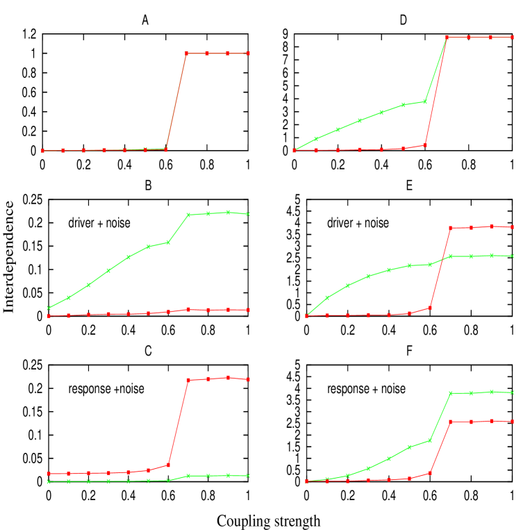
Figure 4: Interdependencies between two Henon systems with equal $b$-parameter, $b_{1}=b_{2}=0.3$ as functions of the coupling strength (panels A and D). In the other panels, white measurement noise has been added either to the driver (panels B, E) or to the response (panels C, F). Left side figures correspond to $S$ and the ones in the right side to $H$. Black lines are the $({\bf Y}|{\bf X})$ interdependencies and grey lines correspond to $({\bf X}|{\bf Y})$.

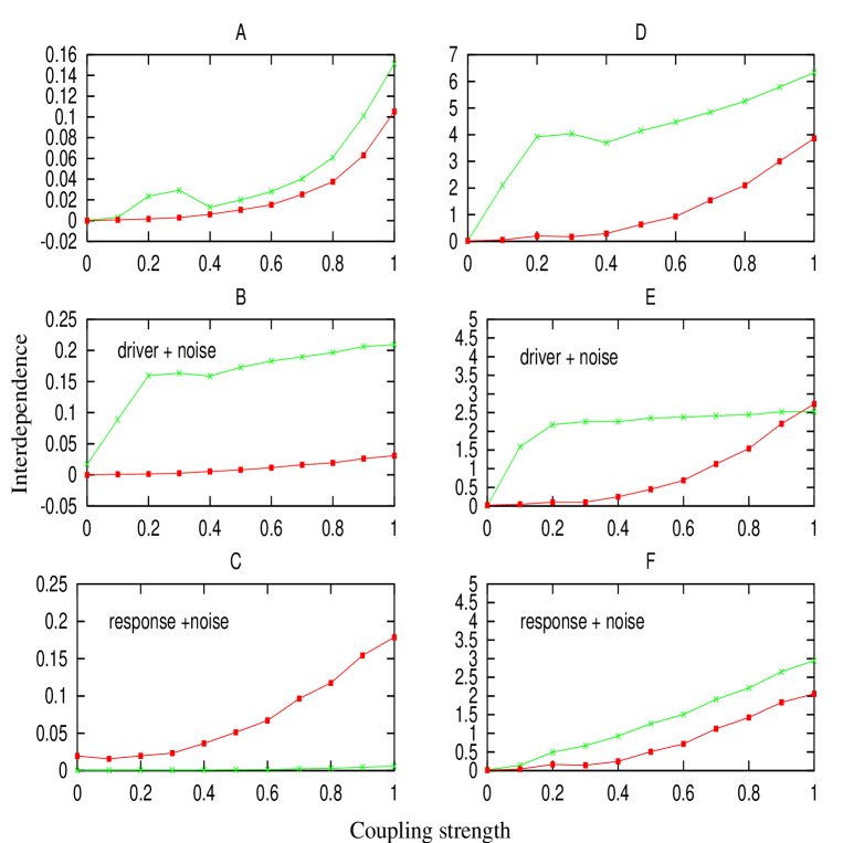
Figure 5: Same as fig.4, with $b_{1}=0.3$, $b_{2}=0.1$.

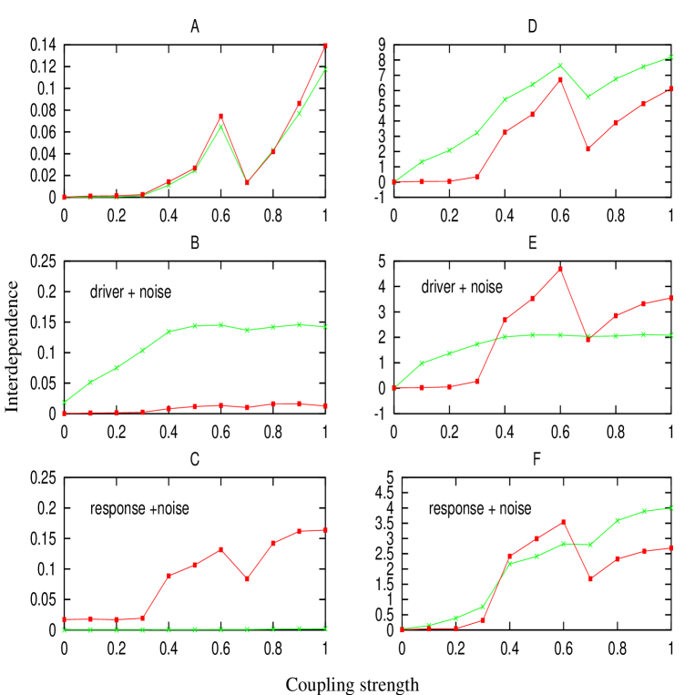
Figure 6: Same as fig.4 with $b_{1}=0.1$, $b_{2}=0.3$. In panel C, the curve for $S({\bf X}|{\bf Y})$ coincides with the x-axis within our precision.

References

- [1] Y. Lei, E. Ott, and Q. Chen, Phys. Rev. Lett. 65, 2935 (1990)
- [2] A. Pikovsky, Phys. Lett. A165, 33 (1992)
- [3] N.F. Rulkov, M.M. Sushchik, L.S. Tsimring, and H.D.I. Abarbanel. Phys. Rev. E 51, 980 (1995).
- [4] H. Fujisaka and T. Yamada, Prog. Theor. Phys. 69, 32 (1983); 76, 582 (1986)
- [5] T. Yamada and H. Fujisaka, Prog. Theor. Phys. 70, 1240 (1984); 72, 885 (1985)
- [6] A. Pikovsky, Z. Physik B 55, 149 (1984).
- [7] H.G. Schuster, S. Martin, and W. Martiensen, Phys Rev. A 33, 3547 (1986)
- [8] L.M. Pecora and T.L. Carroll, Phys. Rev. Lett. 64, 821 (1990).
- [9] A. Pikovsky and P. Grassberger, J. Phys. A 24, 4587 (1991).
- [10] M. Le Van Quyen, J. Martinerie, C. Adam, and F.J. Varela, Physica D 127, 250 (1999).
- [11] H.D.I. Abarbanel, N. Rulkov, and M. Sushchik, Phys. Rev. E 53, 4528 (1996).
- [12] R. Brown and L. Kocarev, E-print chao-dyn/9811013 (1998).
- [13] K. Josić, Phys. Rev. Lett. 80, 3053 (1998).
- [14] K. Pyragas, Phys. Rev. E 54, R4508 (1996).
- [15] B.R. Hunt, E. Ott, and J.A. Yorke, Phys. Rev. E 55, 4029 (1997)
- [16] M. Le Van Quyen, C. Adam, M. Baulac, J. Martenierie, and F.J. Varela, Brain Research 792, 24 (1998).
- [17] S.J. Schiff, P. So, T. Chang, R.E. Burke and T. Sauer. Phys. Rev. E 54, 6708 (1996).
- [18] J. Arnhold, P. Grassberger, K. Lehnertz, and C.E. Elger, Physica D, in press (1999); e-print chao-dyn/9907013.
- [19] R. Brown, Phys. Rev. Lett. 81, 4835 (1998)
- [20] P. Frederickson, J.L. Kaplan, and J.A. Yorke, J. Diff. Eqns. 49, 185 (1983).
- [21] F. Takens, in D.A. Rand and L.S. Young, eds., Lecture Notes in Mathematics 898, page 366 (Springer, Berlin etc., 1981).
- [22] E.N. Lorenz, Nature 353, 241 (1991).