The Scaling Structure of the Velocity Statistics in Atmospheric Boundary Layers

Abstract

The statistical objects characterizing turbulence in real turbulent flows differ from those of the ideal homogeneous isotropic model. They contain contributions from various two-dimensional and three-dimensional aspects, and from the superposition of inhomogeneous and anisotropic contributions. We employ the recently introduced decomposition of statistical tensor objects into irreducible representations of the SO(3) symmetry group (characterized by $j$ and $m$ indices, where $j=0\dots\infty$, $-j\leq m\leq j$) to disentangle some of these contributions, separating the universal and the asymptotic from the specific aspects of the flow. The different $j$ contributions transform differently under rotations and so form a complete basis in which to represent the tensor objects under study. The experimental data are recorded with hot-wire probes placed at various heights in the atmospheric surface layer. Time series data from single probes and from pairs of probes are analyzed to compute the amplitudes and exponents of different contributions to the second order statistical objects characterized by $j=0$, $j=1$ and $j=2$. The analysis shows the need to make a careful distinction between long-lived quasi two-dimensional turbulent motions (close to the ground) and relatively short-lived three-dimensional motions. We demonstrate that the leading scaling exponents in the three leading sectors ($j=0,1,2$) appear to be different but universal, independent of the positions of the probe, the tensorial component considered, and the large scale properties. The measured values of the scaling exponent are $\zeta^{(j=0)}_{2}=0.68\pm 0.01$, $\zeta^{(j=1)}_{2}=1.0\pm 0.15$ and $\zeta^{(j=2)}_{2}=1.38\pm 0.10$. We present theoretical arguments for the values of these exponents using the Clebsch representation of the Euler equations; neglecting anomalous corrections, the values obtained are 2/3, 1 and 4/3 respectively. Some enigmas and questions for the future are sketched.

I Introduction

The atmospheric boundary layer is a natural laboratory of turbulence that is unique in that it offers very high Reynolds numbers (Re). Especially if the measurements are made during periods when mean wind speed and direction are roughly constant, one approaches “controlled” conditions that are the goals of an experiment. Students of turbulence interested in the scaling properties, expected to be universal in the limit Re$\to\infty$, are thus attracted to atmospheric measurements. On the other hand the boundary layer suffers inherently from strong inhomogeneity (explicit dependence of the turbulence statistics on the height) which leads to strong anisotropies such that the vertical and horizontal directions are quite distinguishable. In addition, one may expect the boundary layer near the ground to exhibit large-scale quasi two-dimensional eddies whose typical decay times and statistics may differ significantly from the generic three-dimensional motion. The aim of this paper is to offer systematic methods of analysis to resolve such difficulties, leading to a useful extraction of the universal, three-dimensional aspects of turbulence.

Fundamentally, we propose to anchor the analysis of the statistical objects that are important in turbulence to the irreducible representations of the SO(3) symmetry group. Although the turbulence that we study is non-isotropic, the Navier-Stokes equations are invariant to all rotations. Together with incompressibility, this invariance implies that the hierarchy of dynamical equations satisfied by the correlation or structure functions are also isotropic [1]. This symmetry has been used in [1] to show that every component of the general solution with a given index $j$, and hence a definite behavior under rotation, has to satisfy these equations individually, independent of other components with different behavior under rotation. This “foliation” of the hierarchical equations motivates us to expect different scaling exponents for each component belonging to a particular $j$ sector of the SO(3) decomposition. A preliminary test of these ideas has been reported in [2]. The main result of the analysis shown below, supporting the results in [2], is that in each sector of the symmetry group scaling behavior can be found with apparently universal scaling exponents. We demonstrate below that scale-dependent correlation functions and structure functions can be usefully represented as a sum of contributions with increasing index $j$ characterizing the irreducible representations of SO(3). In such a sum the coefficients are not universal, but the scale dependence is characterized by universal exponents. That is, a general component $S^{\alpha\beta}({\mathchoice{{\hbox{\boldmath$\displaystyle R$}}}{{\hbox{\boldmath$\textstyle R$}}}{{\hbox{\boldmath$\scriptstyle R$}}}{{\hbox{\boldmath$\scriptscriptstyle R$}}}})$ of the second rank structure function,

$$S^{\alpha\beta}({\mathchoice{{\hbox{\boldmath$\displaystyle R$}}}{{\hbox{\boldmath$\textstyle R$}}}{{\hbox{\boldmath$\scriptstyle R$}}}{{\hbox{\boldmath$\scriptscriptstyle R$}}}})\equiv\langle[u^{\alpha}({\mathchoice{{\hbox{\boldmath$\displaystyle x$}}}{{\hbox{\boldmath$\textstyle x$}}}{{\hbox{\boldmath$\scriptstyle x$}}}{{\hbox{\boldmath$\scriptscriptstyle x$}}}}+{\mathchoice{{\hbox{\boldmath$\displaystyle R$}}}{{\hbox{\boldmath$\textstyle R$}}}{{\hbox{\boldmath$\scriptstyle R$}}}{{\hbox{\boldmath$\scriptscriptstyle R$}}}})-u^{\alpha}({\mathchoice{{\hbox{\boldmath$\displaystyle x$}}}{{\hbox{\boldmath$\textstyle x$}}}{{\hbox{\boldmath$\scriptstyle x$}}}{{\hbox{\boldmath$\scriptscriptstyle x$}}}})][u^{\beta}({\mathchoice{{\hbox{\boldmath$\displaystyle x$}}}{{\hbox{\boldmath$\textstyle x$}}}{{\hbox{\boldmath$\scriptstyle x$}}}{{\hbox{\boldmath$\scriptscriptstyle x$}}}}+{\mathchoice{{\hbox{\boldmath$\displaystyle R$}}}{{\hbox{\boldmath$\textstyle R$}}}{{\hbox{\boldmath$\scriptstyle R$}}}{{\hbox{\boldmath$\scriptscriptstyle R$}}}})-u^{\beta}({\mathchoice{{\hbox{\boldmath$\displaystyle x$}}}{{\hbox{\boldmath$\textstyle x$}}}{{\hbox{\boldmath$\scriptstyle x$}}}{{\hbox{\boldmath$\scriptscriptstyle x$}}}})]\rangle\ ,$$ (1)

where $\langle\dots\rangle$ stands for an ensemble average, can be usefully presented as a sum

$$S^{\alpha\beta}({\mathchoice{{\hbox{\boldmath$\displaystyle R$}}}{{\hbox{\boldmath$\textstyle R$}}}{{\hbox{\boldmath$\scriptstyle R$}}}{{\hbox{\boldmath$\scriptscriptstyle R$}}}})=\sum_{q,j,m}a_{qjm}(R)B_{qjm}^{\alpha\beta}(\hat{\mathchoice{{\hbox{\boldmath$\displaystyle R$}}}{{\hbox{\boldmath$\textstyle R$}}}{{\hbox{\boldmath$\scriptstyle R$}}}{{\hbox{\boldmath$\scriptscriptstyle R$}}}})\ ,$$ (2)

where ${\mathchoice{{\hbox{\boldmath$\displaystyle B$}}}{{\hbox{\boldmath$\textstyle B$}}}{{\hbox{\boldmath$\scriptstyle B$}}}{{\hbox{\boldmath$\scriptscriptstyle B$}}}}_{qjm}$ are the basis functions of the SO(3) symmetry group that depend on the direction of $\textstyle R$ and $a_{qjm}$ are the coefficients that depend on the magnitude of $\textstyle R$ and, in general, include any scaling behavior. In other words, in terms of a rotation operator $O_{\Lambda}$ which rotates space by an arbitrary angle $\Lambda$ one writes

$$O_{\Lambda}B^{\alpha\beta}_{qjm}(\hat{\mathchoice{{\hbox{\boldmath$\displaystyle R$}}}{{\hbox{\boldmath$\textstyle R$}}}{{\hbox{\boldmath$\scriptstyle R$}}}{{\hbox{\boldmath$\scriptscriptstyle R$}}}})=\sum_{m^{\prime}=-j}^{+j}D_{m^{\prime}m}^{(j)}(\Lambda)B_{qjm}^{\alpha\beta}(\hat{\mathchoice{{\hbox{\boldmath$\displaystyle R$}}}{{\hbox{\boldmath$\textstyle R$}}}{{\hbox{\boldmath$\scriptstyle R$}}}{{\hbox{\boldmath$\scriptscriptstyle R$}}}})\ .$$ (3)

The $(2j+1)\times(2j+1)$ matrices $D_{m^{\prime}m}^{(j)}$ are the irreducible representations of the SO(3) symmetry group. The index $q$ is required because, in general, there may be more than one independent basis function with the same indices $j$ and $m$. We note that the basis functions ${\mathchoice{{\hbox{\boldmath$\displaystyle B$}}}{{\hbox{\boldmath$\textstyle B$}}}{{\hbox{\boldmath$\scriptstyle B$}}}{{\hbox{\boldmath$\scriptscriptstyle B$}}}}_{qjm}$ depend on the unit vector $\hat{\mathchoice{{\hbox{\boldmath$\displaystyle R$}}}{{\hbox{\boldmath$\textstyle R$}}}{{\hbox{\boldmath$\scriptstyle R$}}}{{\hbox{\boldmath$\scriptscriptstyle R$}}}}$ only, whereas the amplitude coefficients $a_{qjm}(R)$ depend on the magnitude of $\textstyle R$ only. Our main point is that amplitudes scale in the inertial range, exhibiting universal exponents,

$$a_{qjm}(R)\propto R^{\zeta_{2}^{(j)}}\ .$$ (4)

Analyzed by usual log-log plots, a superposition such as (2) may well result in continuously changing slopes, as if there is no scaling. One of our main aims is to stress that the scaling exists, but needs to be revealed by unfolding the various contributions. This approach flushes out the scaling behavior even when the Reynolds number Re is low, as in numerical simulations [3].

Obviously, to isolate tensorial components belonging to sectors other than the isotropic one needs to collect data from more than one probe. In Section 2 we present the experimental configuration and the conditions of measurement, and discuss the nature of the data sets. We demonstrate there that having two probes is actually sufficient to read surprisingly rich information about anisotropic turbulence. We have so far used two types of geometries, one consisting of two probes at the same height above the ground and the other with two probes vertically separated. In both cases the inter-probe separation is orthogonal to the mean wind. The caveat is that we must rely on Taylor’s hypothesis [4] to generate scale-dependent structure functions. In anisotropic flows the validity and optimal use of this method require discussion, and this is done in Section 3. In that Section we also examine the issues concerning 2- and 3-dimensional aspects of the flow pattern, and determine the outer scale $L$ at which three-dimensional scaling behavior ceases to exist. In Section 4 we present the main results of the analysis. We demonstrate that the second-order structure function is best described as a superposition of contributions belonging to different sectors of the SO(3) symmetry group by extracting the coefficients and exponents that appear in the superposition (2). The scaling exponents depend on $j$, and we will demonstrate that they are an increasing function of $j$. For $j=0,1,2$ our data analysis leads to the exponent values $0.68\pm 0.01$, $1.0\pm 0.15$ and $1.38\pm 0.10$ respectively. In Section 5 we present theoretical considerations that determine these exponents neglecting intermittency corrections, based on the Clebsch representation of the Euler equation. Section 6 offers a summary of the principal conclusions, and a discussion of the road ahead.

II The experimental setup

The results presented in this paper are based on two experimental setups, which are denoted throughout as I and II respectively. In both setups the data were acquired over the salt flats in Utah with a long fetch. The site of measurements was chosen to provide steady wind conditions. The surface of the desert was very smooth and even. The measurements were made between 6 PM and 9 PM in a summer season during which nearly neutral stability conditions prevailed. The boundary layer was very similar to that on a smooth flat plate. In set I the data were acquired simultaneously from two single hot-wire probes at a height of 6 m above the ground, with a horizontal separation of 55 cm, nominally orthogonal to the mean wind, see Fig. 1.

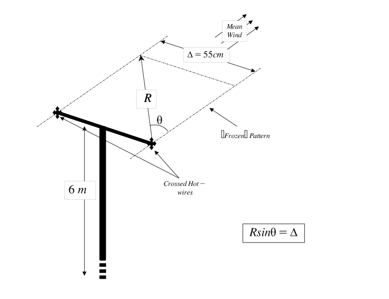
FIG. 1.: Schematic of the experimental set-up. Shown is the positioning of the probes with respect to the mean wind, and an explanation of how Taylor’s hypothesis is employed.

The Taylor microscale Reynolds number was about 10,000. Set II was acquired from an array of three cross-wires, arranged above each other at heights 11 cm, 27 cm and 54 cm respectively. The Taylor microscale Reynolds numbers for this set were 900, 1400 and 2100 respectively. The hot-wires, about 0.7 mm in length and 6 $\mu$m in diameter, were calibrated just prior to mounting them on the mounting posts and checked immediately after dismounting. The hot-wires were operated on DISA 55M01 constant-temperature anemometers. The frequency response of the hot-wires was typically good up to 20 kHz. The voltages from the anemometers were suitably low-pass filtered and digitized. The voltages were constantly monitored on an oscilloscope to ensure that they did not exceed the digitizer limits. The Kolmogorov scales were about 0.75 mm (set I) and 0.5-0.7 mm (set II). Table I lists a few relevant facts about the data records analyzed here. The various symbols have the following meanings: $\overline{U}$ = local mean velocity, $u^{\prime}$ = root-mean-square velocity, $\langle\varepsilon\rangle$ = energy dissipation rate obtained by the assumption of local isotropy and Taylor’s hypothesis, $\eta$ and $\lambda$ are the Kolmogorov scale and Taylor microscale respectively, the microscale Reynolds number $R_{\lambda}\equiv u^{\prime}\lambda/\nu$, and $f_{s}$ is the sampling frequency.

Height	$\overline{U}$	$u^{\prime}$	$10^{2}\langle\varepsilon\rangle$,	$\eta$	$\lambda$	$R_{\lambda}$	$f_{s},$ per	# of
meters	ms-1	ms -1	m 2 s-3	mm	cm		channel, Hz	samples
6	4.1	1.08	$1.1$	0.75	15	10,500	10,000	$4\times 10^{7}$
0.11	2.7	0.47	$6.6$	0.47	2.8	900	5,000	$8\times 10^{6}$
0.27	3.1	0.48	2.8	0.6	4.4	1400	5,000	$8\times 10^{6}$
0.54	3.5	0.5	1.5	0.7	6.2	2100	5,000	$8\times 10^{6}$

TABLE I.: Data sets I (first line) and II (second-fourth lines).

For set I we need to test whether the separation between the two probes is indeed orthogonal to the mean wind. (We do not need to worry about this point in set II, since the probes are above each other). To do so we computed the cross-correlation function $\langle u_{1}(t+\tau)u_{2}(t)\rangle$. Here, $u_{1}$ and $u_{2}$ refer to velocity fluctuations in the direction of the mean wind, for probes 1 and 2 respectively. If the separation were precisely orthogonal to the mean wind, this quantity should be maximum for $\tau=0$. Instead, for set I, we found the maximum shifted slightly to $\tau=0.022$ s, implying that the separation was not precisely orthogonal to the mean wind. To correct for this effect, the data from the second probe were time-shifted by 0.022 s. This amounts to a change in the actual value of the orthogonal distance. We computed this effective distance to be $\Delta\approx 54$ cm (instead of the 55 cm that was set physically). We choose coordinates such that the mean wind direction is along the 3-axis, the vertical is in along the 1-axis and the third direction orthogonal to these is the 2-axis. We denote these directions by the three unit vectors $\hat{\mathchoice{{\hbox{\boldmath$\displaystyle n$}}}{{\hbox{\boldmath$\textstyle n$}}}{{\hbox{\boldmath$\scriptstyle n$}}}{{\hbox{\boldmath$\scriptscriptstyle n$}}}}$, $\hat{\mathchoice{{\hbox{\boldmath$\displaystyle m$}}}{{\hbox{\boldmath$\textstyle m$}}}{{\hbox{\boldmath$\scriptstyle m$}}}{{\hbox{\boldmath$\scriptscriptstyle m$}}}}$, and $\hat{\mathchoice{{\hbox{\boldmath$\displaystyle p$}}}{{\hbox{\boldmath$\textstyle p$}}}{{\hbox{\boldmath$\scriptstyle p$}}}{{\hbox{\boldmath$\scriptscriptstyle p$}}}}$ respectively. The raw data available from set I is $u^{(3)}(t)$ measured at the positions of the two probes. In set II each probe reads a linear combination of $u^{(3)}(t)$ and $u^{(1)}(t)$ from which each component is extractable. From these data we would like to compute the scale-dependent structure functions, using Taylor’s hypothesis to surrogate space for time. This needs a careful discussion, which is given below.

III Theoretical constructs: Taylor’s Hypothesis, Inner and Outer Scales

A Taylor’s Hypothesis

Decades of research on the statistical aspects of hydrodynamic turbulence are based on Taylor’s hypothesis [4-7], which asserts that the fluctuating velocity field measured by a given probe as a function of time, ${\mathchoice{{\hbox{\boldmath$\displaystyle u$}}}{{\hbox{\boldmath$\textstyle u$}}}{{\hbox{\boldmath$\scriptstyle u$}}}{{\hbox{\boldmath$\scriptscriptstyle u$}}}}(t)$, is the same as the velocity ${\mathchoice{{\hbox{\boldmath$\displaystyle u$}}}{{\hbox{\boldmath$\textstyle u$}}}{{\hbox{\boldmath$\scriptstyle u$}}}{{\hbox{\boldmath$\scriptscriptstyle u$}}}}(R/\overline{U})$ where $\overline{U}$ is the mean velocity and $R=-\overline{U}t$ is the distance to a position “upstream” where the velocity is measured at $t=0$. The natural limitation on Taylor’s hypothesis is provided by the typical decay time of fluctuations of scale $R$. Within the classical scaling theory of Kolmogorov, this time scale is the turn-over time $R/\sqrt{S(R)}$ where $S(R)\equiv S^{\alpha\alpha}(R)$. With this estimate, Taylor’s hypothesis is expected to be valid when $\sqrt{S(R)}/\overline{U}\to 0$. Since $S(R)\to 0$ when $R\to 0$, the hypothesis becomes exact in this limit. We will use this aspect to match the units while reading a distance from a combination of space and time intervals.

Reference [7] presents a detailed analysis of the consequences of Taylor’s hypothesis on the basis of an exactly soluble model. It also proposes ways for minimizing the systematic errors introduced by the use of Taylor’s hypothesis. In light of that analysis we will use an “effective” wind, $U_{\rm eff}$, for surrogating the time data. This velocity is a combination of the mean wind $\overline{U}$ and the root-mean-square $u^{\prime}$,

$$U_{\rm eff}\equiv\sqrt{\overline{U}^{2}+(bu^{\prime})^{2}}\ ,$$ (5)

where $b$ is a dimensionless parameter. Evidently, when we employ the Taylor hypothesis in log-log plots of structure functions using time series measured in a single probe, the value of the parameter $b$ is irrelevant, because it merely changes the (arbitrary) units of length (i.e, yields an arbitrary intercept). When we mix real distance between two probes and surrogated distance according to Taylor’s hypothesis, the parameter $b$ becomes a unit fixer. The numerical value of this parameter is found in [7] by the requirement that the surrogated and directly measured structure functions coincide in the limit $R\to 0$. When we do not have the necessary data we will use values of $b$ suggested by the exactly soluble model treated in [7]. This value of $b\approx 3$. We have checked that the scaling exponents change by no more than a few percent upon changing $b$ by 30$\%$. Further, this choice can be justified a posteriori by the quality of the fit of to the predicted scaling functions.

When we have two probes placed at different heights, the mean velocities and $u^{\prime}$ as measured by the probes do not coincide. In applying Taylor’s hypothesis one needs to decide the most appropriate value of $U_{\rm eff}$. This question has been addressed in detail in Ref.[7] with the final conclusion that the choice depends on the velocity profile between the probe. In the case of linear shear the answer is

$$U_{\rm eff}\equiv\sqrt{{\overline{U_{1}}^{2}+\overline{U_{2}}\over 2}^{2}+b{{u_{1}^{\prime}}^{2}+{u_{1}^{\prime}}^{2}\over 2}}\ ,$$ (6)

where the subscripts 1,2 refer to the two probes respectively.

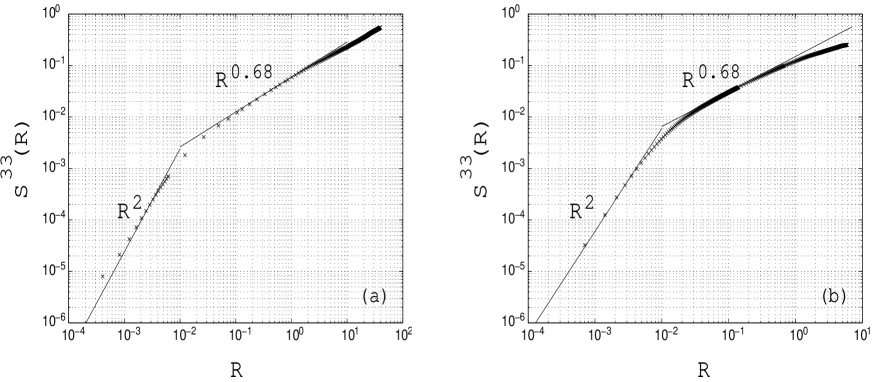
FIG. 2.: Log-log plots of the longitudinal component of the second order structure function. Panel (a) is for data set I and panel (b) for data set II.

In all subsequent expressions, we will therefore denote separations by $R$, and invariably this will mean Taylor-surrogated time differences or a combination of real and Taylor-surrogated distances. The effective velocity will be (5) or (6) depending on whether the probes are at the same height or at different heights.

B Inner and Outer Scales in the Atmospheric Boundary Layer

In seeking scaling behavior one needs to find the inner and outer scales. Below the inner scale second order structure functions have an analytic dependence on the separation, $S(R)\sim R^{2}$, and above the outer scale they should tend to a constant value. We show in Fig. 2 the longitudinal structure functions

$$S^{33}(R)=\langle(u^{(3)}(x+R)-u^{(3)}(x))^{2}\rangle$$ (7)

computed from a single probe in set I and from the probe at $0.54$ m in set II. We also consider in Fig. 3 the transverse structure function

$$S^{11}(R)=\langle(u^{(1)}(x+R)-u^{(1)}(x))^{2}\rangle$$ (8)

computed from the probe at $0.54$ m in set II, see Fig. 3. The spatial scales are computed using the local mean wind in both cases since we do not expect the scaling exponent for the single-probe structure function to be affected by the choice of advection velocity. However, this choice does determine the value of $R$ corresponding to a particular time scale, but we expect that any correction to the numerical value of $R$ is small for a different choice of advection velocity, and not crucial for the qualitative statements that follow. In Fig. 2 we clearly see the $R^{2}$ behavior characterizing the transition from the dissipative to the inertial range. As is well-known [8], this behavior persists for about a half-decade above the “nominal” Kolmogorov length scale $\eta$. There is a region of cross-over and then the isotropic scaling $\sim R^{0.68}$ expected for small scales in the inertial range begins. We thus have no difficulty in identifying the inner scale, it is simply revealed as a natural crossover length in these data.

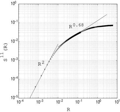
FIG. 3.: Log-log plot of the transverse component of the second order structure function computed from data set II.

Next, since we cannot expect to fit with a single power-law for larger scales and must include scaling contributions due to anisotropy [2], we need to estimate the largest scales that should be included in our fitting procedure using the SO(3) decomposition machinery. We expect that the contributions due to anisotropy will account for scaling behavior up to the outer scale of the three-dimensional flow patterns. The task now is to identify that scale. One approach is simply to use the scale where the longitudinal structure function tends to a constant, corresponding to the scale across which the velocity signal has decorrelated. It becomes immediately apparent that this is not a reasonable estimate of the large scale. Figure 2 shows that the longitudinal structure function stays correlated up to scales that are at least an order of magnitude larger than the height at which the measurement is made. On the other hand, the transverse structure function computed from the probe at $0.54$ m, Fig. 3, ceases to exhibit scaling behavior at a scale that is of the order of the vertical distance of the probe from the ground.

It appears that we are observing extremely flat “quasi-two dimensional” eddies that are correlated over very long distances in the horizontal direction but have a comparatively small vertical velocity component. Accordingly the vertical velocity component is dominated by bona fide three-dimensional turbulence. Since we know that the presence of the boundary must limit the size of the largest three-dimensional structures, the height of the probe should be something of an upper bound on the largest three-dimensional flow patterns that can be detected in experiments. Thus the size of the largest three-dimensional structures is more accurately determined by the decorrelation length of the transverse structure function. The theory of scaling behavior in three-dimensional turbulence can usefully be applied to only those flow patterns that are essentially three-dimensional. The extended flat eddies must be described in terms of a separate theory, including notions of two-dimensional turbulence which has very different scaling properties [9]. This is not the ambition of the present work. Rather, in the following analyses, we choose our outer-scale $L$ in the horizontal direction to be of the order of the decorrelation length of the transverse structure function (where available) or of the height of the probe. We will see below that these two are the same to within a factor of 2; taking $L$ to be as twice the height of the probe is consistent with all our data. We use this estimate in our study of both transverse, longitudinal and mixed objects.

IV Extracting the universal exponents of higher $j$ sectors

In this section we describe a procedure for extracting the scaling exponents that appear in the superposition (2). Preliminary results on the scaling exponent $\zeta_{2}^{(j=2)}$, obtained under the assumption of cylindrical symmetry, were announced in [2]. The analysis here is more complete, and takes into account the full tensorial structure. We show that taking into account the full broken symmetry is feasible, and the final results are essentially the same. Both sets of results are also in agreement with analysis of numerical simulations [3]. The results concerning $\zeta_{2}^{(j=1)}$ are new.

In order to extract a particular $j$ contribution and the associated scaling exponent, one would ideally like to possess the statistics of the velocity at all points in a three-dimensional grid. One could then extract the $j$ contribution of particular interest by multiplying the full structure function by the appropriate $B_{q,j,m}$ and integrating over a sphere of radius $R$. Orthogonality of the basis functions ensures that only the $j$ contribution survives the integration. One could then perform this procedure for various $R$ and extract the scaling behavior. This method was adopted successfully in [3] using data from direct numerical simulations. The experimental data are limited to a few points in space, so the integration over the sphere is not possible. We are faced with a true superposition of contributions from various $j$ sectors with no simple way of disentangling them. However we can do the next best thing and use the postulate that the scaling exponents form a hierarchy of increasing values for increasing $j$. This can be interpreted to mean that anisotropic effects appear to increase with increasing scale. Since we look for the lowest order anisotropic contributions in our analyses, we perform a two-stage procedure to separate the various sectors. First we look at the small scale region of the inertial range to determine the extent of the fit with a single (isotropic) exponent. We then seek to extend this range by including appropriate anisotropic tensor contributions, and obtain the additional scaling exponents using least-squares fitting procedure. The following two sections discuss the procedure for determining the $j=2$ and $j=1$ scaling contributions to second-order statistics.

A The $j$=2 component

In the second order structure function defined already, viz.,

$$S^{\alpha\beta}({{\mathchoice{{\hbox{\boldmath$\displaystyle R$}}}{{\hbox{\boldmath$\textstyle R$}}}{{\hbox{\boldmath$\scriptstyle R$}}}{{\hbox{\boldmath$\scriptscriptstyle R$}}}}})=\langle(u^{\alpha}({{\mathchoice{{\hbox{\boldmath$\displaystyle x$}}}{{\hbox{\boldmath$\textstyle x$}}}{{\hbox{\boldmath$\scriptstyle x$}}}{{\hbox{\boldmath$\scriptscriptstyle x$}}}}}+{{\mathchoice{{\hbox{\boldmath$\displaystyle R$}}}{{\hbox{\boldmath$\textstyle R$}}}{{\hbox{\boldmath$\scriptstyle R$}}}{{\hbox{\boldmath$\scriptscriptstyle R$}}}}})-u^{\alpha}({{\mathchoice{{\hbox{\boldmath$\displaystyle x$}}}{{\hbox{\boldmath$\textstyle x$}}}{{\hbox{\boldmath$\scriptstyle x$}}}{{\hbox{\boldmath$\scriptscriptstyle x$}}}}}))(u^{\beta}({{\mathchoice{{\hbox{\boldmath$\displaystyle x$}}}{{\hbox{\boldmath$\textstyle x$}}}{{\hbox{\boldmath$\scriptstyle x$}}}{{\hbox{\boldmath$\scriptscriptstyle x$}}}}}+{{\mathchoice{{\hbox{\boldmath$\displaystyle R$}}}{{\hbox{\boldmath$\textstyle R$}}}{{\hbox{\boldmath$\scriptstyle R$}}}{{\hbox{\boldmath$\scriptscriptstyle R$}}}}})-u^{\beta}({{\mathchoice{{\hbox{\boldmath$\displaystyle x$}}}{{\hbox{\boldmath$\textstyle x$}}}{{\hbox{\boldmath$\scriptstyle x$}}}{{\hbox{\boldmath$\scriptscriptstyle x$}}}}}))\rangle,$$ (9)

the $j=2$ component of the SO(3) symmetry group corresponds to the lowest order anisotropic contribution that is symmetric in the indices, and has even parity in $\textstyle R$ (due to homogeneity). Although the assumption of axisymmetry used in [2] seemed to be justified from the excellent qualities of fits obtained, we attempt to fit the same data (set I) with the full tensor form for the $j=2$ contribution. The derivation of the full $j=2$ contribution to the symmetric, even parity, structure function appears in Appendix A.

To begin with, we seek the range over which the isotropic scaling exponent holds for data set I. We measure all separation distances in units of $\Delta=0.54$ m which is the distance between the probes. The lower bound to the inertial range in this set is estimated to begin at $R/\Delta\approx 0.2$ (see discussion in Section III B). We then find the range of scales over which the structure function

$$S^{33}(R,\theta=0)=\langle(u_{1}^{(3)}(x+R)-u_{1}^{(3)}(x))^{2}\rangle,$$ (10)

with the subscript $1$ denoting one of the two probes, can be fitted with a single exponent; this then would indicates the limit of isotropic scaling. We find that for points in the range $0.2<R/\Delta<4.5$ a least squares fitting procedure yields a best-fit value $\zeta_{2}=0.68\pm 0.01$ (Fig. 4 (a)). Fig. 4 (b) shows the fit to the structure function computed from a single probe in set I with just the $j=0$ contribution. Above this range, we are unable to obtain a good fit to the data with just the isotropic exponent and Fig. 4 (b) shows the peel-off from isotropic behavior above $R/\Delta\approx 4.5$. We point out that for ranges higher than this, one can indeed able to find a “best-fit” exponent for the curve, but the value of the exponent rapidly decreases and the quality of the fit is compromised.

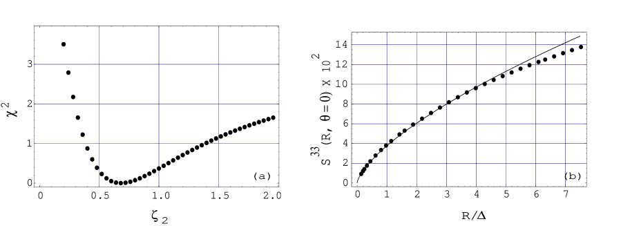
FIG. 4.: The structure function computed from the single probe data, set I. (a) shows the $\chi^{2}$ minimization by the best-fit value of the exponent in the isotropic sector $\zeta_{2}\approx 0.68$ for the single-probe structure function in the range $0.2<R/\Delta<4.5$. (b) shows the fit using the best value of $\zeta_{2}$ obtained in (a), indicating the peel-off from isotropic behavior at the end of the fitted range.

To find the $j=2$ anisotropic exponent we need to use data taken from both probes. To clarify the procedure, we show in Fig. 1 the geometry of set I. What is computed is actually

$$S^{33}(R,\theta)=\langle[u^{(3)}_{1}(U_{\rm eff}t+U_{\rm eff}t_{\tilde{R}})-u^{(3)}_{2}(U_{\rm eff}t)]^{2}\rangle$$ (11)

Here $\theta=\arctan(\Delta/U_{\rm eff}t_{\tilde{R}})$, $t_{\tilde{R}}=\tilde{R}/U_{\rm eff}$, and $R=\sqrt{\Delta^{2}+(\bar{U}_{\rm eff}t_{\tilde{R}})^{2}}$. $U_{\rm eff}$ is defined by Eq. (5) with $b=3$. For simplicity we shall refer from now on to such quantities as

$$S^{33}(R,\theta)=\langle(u_{1}^{(3)}(x+R)-u_{2}^{(3)}(x))^{2}\rangle\ .$$ (12)

Next, we fix the scaling exponent of the isotropic sector as $0.68$ and find the $j=2$ anisotropic exponent that results from fitting to the full $j=2$ tensor contribution. We fit the objects in Eqs. (10) and (12) to the sum of the $j=0$ (with scaling exponent $\zeta_{2}=0.68$) and the $j=2$ contributions (see Appendix A)

$$S^{33}(R,\theta)=S^{33}_{j=0}(R,\theta)+S^{33}_{j=2}(R,\theta)$$ (13)

$$= c_{0}\left({R\over\Delta}\right)^{\zeta_{2}}\Big{[}2+\zeta_{2}-\zeta_{2}\cos^{2}\theta\Big{]}$$ (14)

$$+ a\left({R\over\Delta}\right)^{\zeta_{2}^{(2)}}\Big{[}(\zeta_{2}^{(2)}+2)^{2}-\zeta_{2}^{(2)}(3\zeta_{2}^{(2)}+2)\cos^{2}\theta$$ (15)

$$+ 2\zeta_{2}^{(2)}(\zeta_{2}^{(2)}-2)\cos^{4}\theta\Big{]}$$ (16)

$$+ b\left({R\over\Delta}\right)^{\zeta_{2}^{(2)}}\Big{[}(\zeta_{2}^{(2)}+2)(\zeta_{2}^{(2)}+3)-\zeta_{2}^{(2)}(3\zeta_{2}^{(2)}+4)\cos^{2}\theta$$ (17)

$$+ (2\zeta_{2}^{(2)}+1)(\zeta_{2}^{(2)}-2)\cos^{4}\theta\Big{]}$$ (18)

$$+ a_{9,2,1}\left({R\over\Delta}\right)^{\zeta_{2}^{(2)}}\Big{[}-2\zeta_{2}^{(2)}(\zeta_{2}^{(2)}+2)\sin\theta\cos\theta+2\zeta_{2}^{(2)}(\zeta_{2}^{(2)}-2)\cos^{3}\theta\sin\theta\Big{]}$$ (19)

$$+ a_{9,2,2}\left({R\over\Delta}\right)^{\zeta_{2}^{(2)}}\Big{[}-2\zeta_{2}^{(2)}(\zeta_{2}^{(2)}-2)\cos^{2}\theta\sin^{2}\theta\Big{]}$$ (20)

$$+ a_{1,2,2}\left({R\over\Delta}\right)^{\zeta_{2}^{(2)}}\Big{[}-2\zeta_{2}^{(2)}(\zeta_{2}^{(2)}-2)\sin^{2}\theta\Big{]}.$$ (21)

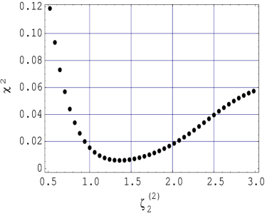
FIG. 5.: The $\chi^{2}$ minimization by the best-fit value of the exponent in the $j=2$ anisotropic sector from the fit to both the $\theta=0$ and the $\theta$-dependent structure functions in the ranges $0.2<R/\Delta<25$ and $1<R/\Delta<25$ respectively.

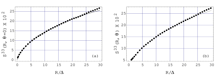
FIG. 6.: The structure functions computed ¿from data set I and fit with the $j=0$ and full $j=2$ tensor contributions using the best fit values of exponents $\zeta_{2}=0.68$ and $\zeta_{2}^{(2)}=1.38$. Panel (a) shows the fit to the single-probe ($\theta=0$) structure function in the range $0.2<R/\Delta<25$ and panel (b) shows the fit to the $\theta$-dependent structure function in the range $1<R/\Delta<25$.

We fit the experimentally generated functions to the above form using values of $\zeta_{2}^{(2)}$ ranging from $0.5$ to $3$. Each iteration of the fitting procedure involves solving for the six unknown, non-universal coefficients. The best value of $\zeta_{2}^{(2)}$ is the one that minimizes the $\chi^{2}$ for these fits; from Fig. 5 we obtain this to be $1.38\pm 0.15$. The fits with this choice of exponent are displayed in Fig. 6. The corresponding values of the six fitted coefficients is given in Table II. The range of scales that are fitted to this expression is $0.2<R/\Delta<25$ for the $\theta=0$ (single-probe) structure function and $1<R/\Delta<25$ for the $\theta\neq 0$ (two-probe) structure function. We are unable to fit with Eq. (21) to larger scales — that is, larger than about 12 meters — without losing the quality of the fit in the small scales. This is roughly twice the height of the probe from the ground. Based on the discussion in Sect. II C, we should be in the regime of the largest scales where the three-dimensional theory would hold. Therefore this limit to the fitting range is consistent with our expectations for the maximum scale of three-dimensional turbulence. We conclude that the structure functions exhibits scaling behavior over the whole scaling range, but this important fact is missed if one does not consider a superposition of the $j=0$ and $j=2$ contributions.

$\zeta_{2}$	$\zeta_{2}^{(2)}$	$c_{0}\times 10^{3}$	$a\times 10^{3}$	$b\times 10^{3}$	$a_{9,2,1}\times 10^{3}$	$a_{9,2,2}\times 10^{3}$	$a_{1,2,2}\times 10^{3}$
0.68	1.38 $\pm 0.10$	7 $\pm 0.5$	-3.2 $\pm$ 0.3	2.6 $\pm$0.3	-0.14$\pm$ 0.02	-5.6 $\pm$ 0.7	-4 $\pm$ 0.5

TABLE II.: The scaling exponents and the 6 coefficients in units of (m/sec)² as determined from the nonlinear fit of Eq. 7 to data set I.

We thus conclude that the estimate for the $j=2$ scaling exponent $\zeta_{2}^{(2)}\approx 1.38$. This same estimate was obtained in [2] using only the axisymmetric terms. The value of the coefficients $a$ and $b$ are again close in magnitude but opposite in sign — just as in [2] giving a small contribution to $S^{33}(R,\theta=0)$. The non-axisymmetric contributions vanish in the case of $\theta=0$. The contribution of these terms to the finite $\theta$ function is relatively small because the angular dependence appears as $\sin\theta$ and $\sin^{2}\theta$, both of which are small for small $\theta$ (large $R$); and hence previously we were able to obtain a good fit to just the axisymmetric contribution. Lastly, we note that the total number of free parameters in this fit is 7 (6 coefficients and 1 exponent). This brings up the possibility of having “over-fit” the data. The relative “flatness” of the $\chi^{2}$ function near its minimum in Fig. 5 could be indicative of the large number of free parameters in the fit. However, the value of the exponent is perfectly in agreement with the analysis of numerical simulations [3] in which one can properly integrate the structure function against the basis functions, eliminating all contributions except that of the $j=2$ sector. Furthermore, fits to the data in the vicinity of $\zeta_{2}^{(2)}=1.38$ show enough divergence from experiment that we are satisfied about the genuineness of the $\chi^{2}$ result.

B Extracting the j=1 component

The homogeneous structure function defined in Eq. (9) is known from properties of symmetry and parity to possess no contribution from the $j=1$ sector (see Appendix B, Section 2), the $j=2$ sector being its lowest order anisotropic contributor. In order to isolate the scaling behavior of the $j=1$ contribution in atmospheric shear flows we must either explicitly construct a new tensor object which will allow for such a contribution, or extract it from the structure function itself computed in the presence of inhomogeneity. In the former case, we construct the tensor

$$T^{\alpha\beta}({{\mathchoice{{\hbox{\boldmath$\displaystyle R$}}}{{\hbox{\boldmath$\textstyle R$}}}{{\hbox{\boldmath$\scriptstyle R$}}}{{\hbox{\boldmath$\scriptscriptstyle R$}}}}})=\langle u^{\alpha}({{\mathchoice{{\hbox{\boldmath$\displaystyle x$}}}{{\hbox{\boldmath$\textstyle x$}}}{{\hbox{\boldmath$\scriptstyle x$}}}{{\hbox{\boldmath$\scriptscriptstyle x$}}}}}+{{\mathchoice{{\hbox{\boldmath$\displaystyle R$}}}{{\hbox{\boldmath$\textstyle R$}}}{{\hbox{\boldmath$\scriptstyle R$}}}{{\hbox{\boldmath$\scriptscriptstyle R$}}}}})-u^{\alpha}({{\mathchoice{{\hbox{\boldmath$\displaystyle x$}}}{{\hbox{\boldmath$\textstyle x$}}}{{\hbox{\boldmath$\scriptstyle x$}}}{{\hbox{\boldmath$\scriptscriptstyle x$}}}}}))(u^{\beta}({{\mathchoice{{\hbox{\boldmath$\displaystyle x$}}}{{\hbox{\boldmath$\textstyle x$}}}{{\hbox{\boldmath$\scriptstyle x$}}}{{\hbox{\boldmath$\scriptscriptstyle x$}}}}}+{{\mathchoice{{\hbox{\boldmath$\displaystyle R$}}}{{\hbox{\boldmath$\textstyle R$}}}{{\hbox{\boldmath$\scriptstyle R$}}}{{\hbox{\boldmath$\scriptscriptstyle R$}}}}})+u^{\beta}({{\mathchoice{{\hbox{\boldmath$\displaystyle x$}}}{{\hbox{\boldmath$\textstyle x$}}}{{\hbox{\boldmath$\scriptstyle x$}}}{{\hbox{\boldmath$\scriptscriptstyle x$}}}}}))\rangle.$$ (22)

This object vanishes both when $\alpha=\beta$ and when $\textstyle R$ is in the direction of homogeneity. ¿From data set II we can calculate this function for non-homogeneous scale-separations (in the shear direction). In general, this will exhibit mixed parity and symmetry; we cannot use the incompressibility condition to reduce our parameter space. Therefore, to minimize the final number of fitting parameters, we examine only the antisymmetric contribution. We derive the tensor contributions in the $j=1$ sector for the antisymmetric case in Appendix B, Section 1, and use this to fit for the unknown $j=1$ exponent. We describe the results of this analysis below. For completeness, we have derived the tensor contributions in the $j=1$ sector for the symmetric case as well in Appendix B2. This can be used to find $j=1$ exponent for the inhomogenous structure function which is symmetric but has mixed parity. We do not present the results of that analysis here essentially because they are consistent with those from the antisymmetric case.

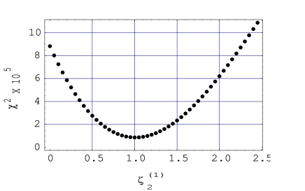
FIG. 7.: The $\chi^{2}$ minimization by the best-fit value of the exponent $\zeta_{2}^{(1)}$ of the $j=1$ anisotropic sector from the fit to $\theta$-dependent ${\widetilde{T}}^{31}(R,\theta)$ function in the range $1<R/\Delta<2.2$.

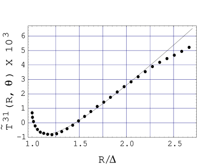
FIG. 8.: The fitted ${\widetilde{T}}^{31}(R,\theta)$ function. The dots indicate the data and the line is the fit.

Returning now to consideration of the antisymmetric part of the tensor object defined in Eq. (22), viz.,

$${\widetilde{T}}^{\alpha\beta}({{\mathchoice{{\hbox{\boldmath$\displaystyle R$}}}{{\hbox{\boldmath$\textstyle R$}}}{{\hbox{\boldmath$\scriptstyle R$}}}{{\hbox{\boldmath$\scriptscriptstyle R$}}}}})={T^{\alpha\beta}({{\mathchoice{{\hbox{\boldmath$\displaystyle R$}}}{{\hbox{\boldmath$\textstyle R$}}}{{\hbox{\boldmath$\scriptstyle R$}}}{{\hbox{\boldmath$\scriptscriptstyle R$}}}}})-T^{\beta\alpha}({{\mathchoice{{\hbox{\boldmath$\displaystyle R$}}}{{\hbox{\boldmath$\textstyle R$}}}{{\hbox{\boldmath$\scriptstyle R$}}}{{\hbox{\boldmath$\scriptscriptstyle R$}}}}})\over 2}=\langle u^{\alpha}({{\mathchoice{{\hbox{\boldmath$\displaystyle x$}}}{{\hbox{\boldmath$\textstyle x$}}}{{\hbox{\boldmath$\scriptstyle x$}}}{{\hbox{\boldmath$\scriptscriptstyle x$}}}}})u^{\beta}({{\mathchoice{{\hbox{\boldmath$\displaystyle x$}}}{{\hbox{\boldmath$\textstyle x$}}}{{\hbox{\boldmath$\scriptstyle x$}}}{{\hbox{\boldmath$\scriptscriptstyle x$}}}}}+{{\mathchoice{{\hbox{\boldmath$\displaystyle R$}}}{{\hbox{\boldmath$\textstyle R$}}}{{\hbox{\boldmath$\scriptstyle R$}}}{{\hbox{\boldmath$\scriptscriptstyle R$}}}}})\rangle-\langle u^{\beta}({{\mathchoice{{\hbox{\boldmath$\displaystyle x$}}}{{\hbox{\boldmath$\textstyle x$}}}{{\hbox{\boldmath$\scriptstyle x$}}}{{\hbox{\boldmath$\scriptscriptstyle x$}}}}})u^{\alpha}({{\mathchoice{{\hbox{\boldmath$\displaystyle x$}}}{{\hbox{\boldmath$\textstyle x$}}}{{\hbox{\boldmath$\scriptstyle x$}}}{{\hbox{\boldmath$\scriptscriptstyle x$}}}}}+{{\mathchoice{{\hbox{\boldmath$\displaystyle R$}}}{{\hbox{\boldmath$\textstyle R$}}}{{\hbox{\boldmath$\scriptstyle R$}}}{{\hbox{\boldmath$\scriptscriptstyle R$}}}}})\rangle,$$ (23)

which will only have contributions from the antisymmetric $j=1$ basis tensors. An additional useful property of this object is that, it does not have any contribution from the isotropic $j=0$ sector spanned by $\delta^{\alpha\beta}$ and $R^{\alpha}R^{\beta}$. This allows us to isolate the $j=1$ contribution and determine its scaling exponent $\zeta_{2}^{(1)}$ starting from the smallest scales available. Using data (set II) from the probes at $0.27$ m (probe 1) and at $0.11$ m (probe 2) we calculate

$${\widetilde{T}}^{31}({{\mathchoice{{\hbox{\boldmath$\displaystyle R$}}}{{\hbox{\boldmath$\textstyle R$}}}{{\hbox{\boldmath$\scriptstyle R$}}}{{\hbox{\boldmath$\scriptscriptstyle R$}}}}})=\langle u_{2}^{(3)}({\mathchoice{{\hbox{\boldmath$\displaystyle x$}}}{{\hbox{\boldmath$\textstyle x$}}}{{\hbox{\boldmath$\scriptstyle x$}}}{{\hbox{\boldmath$\scriptscriptstyle x$}}}})u_{1}^{(1)}({\mathchoice{{\hbox{\boldmath$\displaystyle x$}}}{{\hbox{\boldmath$\textstyle x$}}}{{\hbox{\boldmath$\scriptstyle x$}}}{{\hbox{\boldmath$\scriptscriptstyle x$}}}}+{\mathchoice{{\hbox{\boldmath$\displaystyle R$}}}{{\hbox{\boldmath$\textstyle R$}}}{{\hbox{\boldmath$\scriptstyle R$}}}{{\hbox{\boldmath$\scriptscriptstyle R$}}}})\rangle-\langle u_{1}^{(3)}({\mathchoice{{\hbox{\boldmath$\displaystyle x$}}}{{\hbox{\boldmath$\textstyle x$}}}{{\hbox{\boldmath$\scriptstyle x$}}}{{\hbox{\boldmath$\scriptscriptstyle x$}}}}+{\mathchoice{{\hbox{\boldmath$\displaystyle R$}}}{{\hbox{\boldmath$\textstyle R$}}}{{\hbox{\boldmath$\scriptstyle R$}}}{{\hbox{\boldmath$\scriptscriptstyle R$}}}})u_{2}^{(1)}({\mathchoice{{\hbox{\boldmath$\displaystyle x$}}}{{\hbox{\boldmath$\textstyle x$}}}{{\hbox{\boldmath$\scriptstyle x$}}}{{\hbox{\boldmath$\scriptscriptstyle x$}}}})\rangle\ ,$$ (24)

where again superscripts denote the velocity component and subscripts denote the probe by which this component is measured. The goal is to fit this experimental object to the tensor form derived in Appendix B1, Eq. (B7),

$${\widetilde{T}}^{31}(R,\theta,\phi=0)=-a_{3,1,0}R^{\zeta_{2}^{(1)}}\sin\theta+a_{2,1,1}R^{\zeta_{2}^{(1)}}+a_{3,1,-1}R^{\zeta_{2}^{(1)}}\cos\theta.$$ (25)

Figure 7 gives the $\chi^{2}$ minimization of the fit as a function of $\zeta_{2}^{(1)}$. We obtain the best value to be $1\pm 0.15$ for the final fit. This is shown in Fig. 8. The fit in Fig. 8 peels off at around $R/\Delta=2$. The values of the coefficients corresponding to the exponent $\zeta_{2}^{(1)}=1$ are given in Table III. The maximum range of scales over which the fit works is of the order of the height of the probes from the ground, consistent with the considerations presented earlier. This value of the scaling exponent of the $j=1$ sector is entirely new. Again, we have satisfied ourselves that a different value of the exponent yields a substantially poorer fit to the data.

In Section 5 we will present theoretical considerations to show that the value $\zeta_{2}^{(1)}=1$ is predicted by a version of classical dimensional analysis. The present findings significantly strengthen our proposition [1] that the scaling exponents in the various sectors (at least up to $j=2$) are indeed universal.

$\zeta_{2}^{(1)}$	$a_{3,1,0}$	$a_{2,1,1}$	$a_{3,1,-1}$
$1\pm 0.15$	$0.0116\pm 0.001$	$0.0124\pm 0.001$	$-0.0062\pm 0.001$

TABLE III.: The values of the exponents and coefficients (in units of (m/sec)²) obtained from the fit to the function ${\widetilde{T}}^{31}(R,\theta)$.

V Theoretical determination of $\zeta_{2}^{(j)}$ for $j=1,2$

In this section we present dimensional considerations to determine the “classical K41” values expected of $\zeta_{2}^{(1)}$ and $\zeta_{2}^{(2)}$. We work at the same level as the K41 approach that yields the value $\zeta_{2}^{(0)}=2/3$. This is justified since the differences between any two values $\zeta_{2}^{(j)}$ and $\zeta_{2}^{(j^{\prime})}$ for $j\neq j^{\prime}$ are considerably larger than the intermittency corrections to either of them. We note, however, that the issue of anomalous exponents in turbulence has now multiplied several-fold, to all the $j$ sectors, in light of the apparent universality that has unfolded in this work.

It is easiest to produce a dimensional estimate for $\zeta_{2}^{(2)}$. One simply asserts [5] that the $j=2$ contribution is the first one appearing in $S^{\alpha\beta}({\mathchoice{{\hbox{\boldmath$\displaystyle R$}}}{{\hbox{\boldmath$\textstyle R$}}}{{\hbox{\boldmath$\scriptstyle R$}}}{{\hbox{\boldmath$\scriptscriptstyle R$}}}})$ due to the existence of a shear. Since the shear is a second rank tensor, it can appear linearly in the $j=2$ contribution to $S^{\alpha\beta}({\mathchoice{{\hbox{\boldmath$\displaystyle R$}}}{{\hbox{\boldmath$\textstyle R$}}}{{\hbox{\boldmath$\scriptstyle R$}}}{{\hbox{\boldmath$\scriptscriptstyle R$}}}})$. We thus write for any $m$, $-j\leq m\leq j$,

$$S_{j=2}^{\alpha\beta}({\mathchoice{{\hbox{\boldmath$\displaystyle R$}}}{{\hbox{\boldmath$\textstyle R$}}}{{\hbox{\boldmath$\scriptstyle R$}}}{{\hbox{\boldmath$\scriptscriptstyle R$}}}})\sim T^{\alpha\beta\gamma\delta}{\partial\bar{U}^{\gamma}\over\partial r^{\delta}}f(R,\bar{\epsilon})\ ,$$ (26)

Here $T^{\alpha\beta\gamma\delta}$ is a constant dimensionless tensor made of $\delta^{\alpha\beta}$, $R^{\alpha}/R$, and bilinear contributions made of the three unit vectors $\hat{\mathchoice{{\hbox{\boldmath$\displaystyle p$}}}{{\hbox{\boldmath$\textstyle p$}}}{{\hbox{\boldmath$\scriptstyle p$}}}{{\hbox{\boldmath$\scriptscriptstyle p$}}}},~{}\hat{\mathchoice{{\hbox{\boldmath$\displaystyle m$}}}{{\hbox{\boldmath$\textstyle m$}}}{{\hbox{\boldmath$\scriptstyle m$}}}{{\hbox{\boldmath$\scriptscriptstyle m$}}}},~{}\hat{\mathchoice{{\hbox{\boldmath$\displaystyle n$}}}{{\hbox{\boldmath$\textstyle n$}}}{{\hbox{\boldmath$\scriptstyle n$}}}{{\hbox{\boldmath$\scriptscriptstyle n$}}}}$, as exemplified in appendix A. The way Eq.(26) is represented means that the dimensional function $f(R,\bar{\epsilon})$ stands for the response of the second order structure function to a small external shear. Ad such it is an inherent property of isotropic turbulence. Within the standard Kolomogorov-41 dimensional reasoning this function in the inertial interval can be made only of the mean energy flux per unit time and mass, $\bar{\epsilon}$ and $R$ itself. The only combination of $\bar{\epsilon}$ and $R$ that yields the right dimensions of the function $f$ is $\bar{\epsilon}^{1/3}R^{4/3}$. Therefore

$$S_{j=2}^{\alpha\beta}({\mathchoice{{\hbox{\boldmath$\displaystyle R$}}}{{\hbox{\boldmath$\textstyle R$}}}{{\hbox{\boldmath$\scriptstyle R$}}}{{\hbox{\boldmath$\scriptscriptstyle R$}}}})\sim T^{\alpha\beta\gamma\delta}{\partial\bar{U}^{\gamma}\over\partial r^{\delta}}\bar{\epsilon}^{1/3}R^{4/3}\ .$$ (27)

We thus find a “classical K41” value of $\zeta_{2}^{(2)}=4/3$. Thus this simple argument seems to rationalize nicely the experimentally found value $\zeta_{2}^{(2)}=1.38\pm 0.1$.

To understand the value of $\zeta_{2}^{(1)}$ we cannot proceed in the same way. We need a contribution that is linear (rather than bilinear) in the unit vectors $\hat{\mathchoice{{\hbox{\boldmath$\displaystyle p$}}}{{\hbox{\boldmath$\textstyle p$}}}{{\hbox{\boldmath$\scriptstyle p$}}}{{\hbox{\boldmath$\scriptscriptstyle p$}}}},~{}\hat{\mathchoice{{\hbox{\boldmath$\displaystyle m$}}}{{\hbox{\boldmath$\textstyle m$}}}{{\hbox{\boldmath$\scriptstyle m$}}}{{\hbox{\boldmath$\scriptscriptstyle m$}}}},~{}\hat{\mathchoice{{\hbox{\boldmath$\displaystyle n$}}}{{\hbox{\boldmath$\textstyle n$}}}{{\hbox{\boldmath$\scriptstyle n$}}}{{\hbox{\boldmath$\scriptscriptstyle n$}}}}$. We cannot construct a contribution that is linear in the shear and yet does not vanish due to the incompressibility constraint. Thus there is a fundamental difference between the $j=2$ contribution and the $j=1$ term. While the former can be understood as an inhomogeneous term linear in the forced shear, the $j=1$ term, being more subtle, may be connected to a solution of some homogeneous equation well within the inertial interval. In fact, all the known inertial-interval spectra in turbulent systems are related to the existence of a a flux of some conserved quantity which has a representation as an integral of some density in $\textstyle k$-space. For example the kinetic energy may be written as $\int d{\mathchoice{{\hbox{\boldmath$\displaystyle k$}}}{{\hbox{\boldmath$\textstyle k$}}}{{\hbox{\boldmath$\scriptstyle k$}}}{{\hbox{\boldmath$\scriptscriptstyle k$}}}}|{\mathchoice{{\hbox{\boldmath$\displaystyle u$}}}{{\hbox{\boldmath$\textstyle u$}}}{{\hbox{\boldmath$\scriptstyle u$}}}{{\hbox{\boldmath$\scriptscriptstyle u$}}}}({\mathchoice{{\hbox{\boldmath$\displaystyle k$}}}{{\hbox{\boldmath$\textstyle k$}}}{{\hbox{\boldmath$\scriptstyle k$}}}{{\hbox{\boldmath$\scriptscriptstyle k$}}}},t)|^{2}$. A well-known other integral of motion in hydrodynamics with such a presentations is the helicity

$$H=\int d{\mathchoice{{\hbox{\boldmath$\displaystyle r$}}}{{\hbox{\boldmath$\textstyle r$}}}{{\hbox{\boldmath$\scriptstyle r$}}}{{\hbox{\boldmath$\scriptscriptstyle r$}}}}\,\big{(}{\mathchoice{{\hbox{\boldmath$\displaystyle u$}}}{{\hbox{\boldmath$\textstyle u$}}}{{\hbox{\boldmath$\scriptstyle u$}}}{{\hbox{\boldmath$\scriptscriptstyle u$}}}}\cdot{\mathchoice{{\hbox{\boldmath$\displaystyle\nabla$}}}{{\hbox{\boldmath$\textstyle\nabla$}}}{{\hbox{\boldmath$\scriptstyle\nabla$}}}{{\hbox{\boldmath$\scriptscriptstyle\nabla$}}}}\times{\mathchoice{{\hbox{\boldmath$\displaystyle u$}}}{{\hbox{\boldmath$\textstyle u$}}}{{\hbox{\boldmath$\scriptstyle u$}}}{{\hbox{\boldmath$\scriptscriptstyle u$}}}}\big{)}\ .$$ (28)

Thus the helicity may be considered as a natural candidate which is responsible for a new solution in the inertial interval that may rationalize the $j=1$ finding. We show that this is not the case in the following way.

The dimensionality of $H$ (denoted as [$H$]) differs from the dimensionality of the energy $E$ by one length: $[H]=[E/R]$. Correspondingly, the dimensionality of the helicity flux, $\bar{h}$ may be written as

$$[\bar{h}]=[\bar{\epsilon}/R]\ .$$ (29)

It means that in turbulence with energy and helicity fluxes one has at one’s disposal a dimensionless factor in the form $\bar{h}\,R/\bar{\epsilon}$. It means that the second order structure function ${\mathchoice{{\hbox{\boldmath$\displaystyle S$}}}{{\hbox{\boldmath$\textstyle S$}}}{{\hbox{\boldmath$\scriptstyle S$}}}{{\hbox{\boldmath$\scriptscriptstyle S$}}}}(R,\bar{\epsilon},\bar{h})$ cannot be found just by dimensional reasoning even within the K41 approach. Nevertheless, assuming that at small helicity fluxes (i.e. when $\bar{h}\,R/\bar{\epsilon}\ll 1$) the function ${\mathchoice{{\hbox{\boldmath$\displaystyle S$}}}{{\hbox{\boldmath$\textstyle S$}}}{{\hbox{\boldmath$\scriptstyle S$}}}{{\hbox{\boldmath$\scriptscriptstyle S$}}}}(R,\bar{\epsilon},\bar{h})$ may be expanded in powers of $\bar{h}$ we can justify the first order correction due to helicity, $\delta_{h}{\mathchoice{{\hbox{\boldmath$\displaystyle S$}}}{{\hbox{\boldmath$\textstyle S$}}}{{\hbox{\boldmath$\scriptstyle S$}}}{{\hbox{\boldmath$\scriptscriptstyle S$}}}}$, as

$$\delta_{h}{\mathchoice{{\hbox{\boldmath$\displaystyle S$}}}{{\hbox{\boldmath$\textstyle S$}}}{{\hbox{\boldmath$\scriptstyle S$}}}{{\hbox{\boldmath$\scriptscriptstyle S$}}}}(R,\bar{\epsilon},\bar{h})\sim(\bar{\epsilon})^{-1/3}\bar{h}R^{5/3}\ .$$ (30)

The value of the inferred scaling exponent, i.e. 5/3, is much larger than the value unity found experimentally. We thus need to find another invariant that may rationalize the findings.

The only invariance in addition to the conservation of helicity that we are aware of in the inviscid limit is the Kelvin circulation theorem, which however does not furnish a local integral in $\textstyle k$-space in the Eulerian representation. The only way that is apparent to us to expose this invariance in a useful way is the Clebsch representation, in which one writes the Euler equation in terms of one complex field $a({\mathchoice{{\hbox{\boldmath$\displaystyle r$}}}{{\hbox{\boldmath$\textstyle r$}}}{{\hbox{\boldmath$\scriptstyle r$}}}{{\hbox{\boldmath$\scriptscriptstyle r$}}}},t)$, see for example[10]. In $\textstyle k$-representation the Fourier component of the velocity field ${\mathchoice{{\hbox{\boldmath$\displaystyle u$}}}{{\hbox{\boldmath$\textstyle u$}}}{{\hbox{\boldmath$\scriptstyle u$}}}{{\hbox{\boldmath$\scriptscriptstyle u$}}}}({\mathchoice{{\hbox{\boldmath$\displaystyle k$}}}{{\hbox{\boldmath$\textstyle k$}}}{{\hbox{\boldmath$\scriptstyle k$}}}{{\hbox{\boldmath$\scriptscriptstyle k$}}}},t)$ is determined from a bilinear combination of the complex field:

$${\mathchoice{{\hbox{\boldmath$\displaystyle u$}}}{{\hbox{\boldmath$\textstyle u$}}}{{\hbox{\boldmath$\scriptstyle u$}}}{{\hbox{\boldmath$\scriptscriptstyle u$}}}}({\mathchoice{{\hbox{\boldmath$\displaystyle k$}}}{{\hbox{\boldmath$\textstyle k$}}}{{\hbox{\boldmath$\scriptstyle k$}}}{{\hbox{\boldmath$\scriptscriptstyle k$}}}},t) = \frac{1}{8\pi^{3}}\int d^{3}k_{1}d^{3}k_{2}{\mathchoice{{\hbox{\boldmath$\displaystyle\Psi$}}}{{\hbox{\boldmath$\textstyle\Psi$}}}{{\hbox{\boldmath$\scriptstyle\Psi$}}}{{\hbox{\boldmath$\scriptscriptstyle\Psi$}}}}({\mathchoice{{\hbox{\boldmath$\displaystyle k$}}}{{\hbox{\boldmath$\textstyle k$}}}{{\hbox{\boldmath$\scriptstyle k$}}}{{\hbox{\boldmath$\scriptscriptstyle k$}}}}_{1},{\mathchoice{{\hbox{\boldmath$\displaystyle k$}}}{{\hbox{\boldmath$\textstyle k$}}}{{\hbox{\boldmath$\scriptstyle k$}}}{{\hbox{\boldmath$\scriptscriptstyle k$}}}}_{2})a^{*}({\mathchoice{{\hbox{\boldmath$\displaystyle k$}}}{{\hbox{\boldmath$\textstyle k$}}}{{\hbox{\boldmath$\scriptstyle k$}}}{{\hbox{\boldmath$\scriptscriptstyle k$}}}}_{1},t)a({\mathchoice{{\hbox{\boldmath$\displaystyle k$}}}{{\hbox{\boldmath$\textstyle k$}}}{{\hbox{\boldmath$\scriptstyle k$}}}{{\hbox{\boldmath$\scriptscriptstyle k$}}}}_{2},t)\ ,$$ (31)

$${\mathchoice{{\hbox{\boldmath$\displaystyle\Psi$}}}{{\hbox{\boldmath$\textstyle\Psi$}}}{{\hbox{\boldmath$\scriptstyle\Psi$}}}{{\hbox{\boldmath$\scriptscriptstyle\Psi$}}}}({\mathchoice{{\hbox{\boldmath$\displaystyle k$}}}{{\hbox{\boldmath$\textstyle k$}}}{{\hbox{\boldmath$\scriptstyle k$}}}{{\hbox{\boldmath$\scriptscriptstyle k$}}}}_{1},{\mathchoice{{\hbox{\boldmath$\displaystyle k$}}}{{\hbox{\boldmath$\textstyle k$}}}{{\hbox{\boldmath$\scriptstyle k$}}}{{\hbox{\boldmath$\scriptscriptstyle k$}}}}_{2}) = \frac{1}{2}\left({\mathchoice{{\hbox{\boldmath$\displaystyle k$}}}{{\hbox{\boldmath$\textstyle k$}}}{{\hbox{\boldmath$\scriptstyle k$}}}{{\hbox{\boldmath$\scriptscriptstyle k$}}}}_{1}+{\mathchoice{{\hbox{\boldmath$\displaystyle k$}}}{{\hbox{\boldmath$\textstyle k$}}}{{\hbox{\boldmath$\scriptstyle k$}}}{{\hbox{\boldmath$\scriptscriptstyle k$}}}}_{2}-({\mathchoice{{\hbox{\boldmath$\displaystyle k$}}}{{\hbox{\boldmath$\textstyle k$}}}{{\hbox{\boldmath$\scriptstyle k$}}}{{\hbox{\boldmath$\scriptscriptstyle k$}}}}_{1}-{\mathchoice{{\hbox{\boldmath$\displaystyle k$}}}{{\hbox{\boldmath$\textstyle k$}}}{{\hbox{\boldmath$\scriptstyle k$}}}{{\hbox{\boldmath$\scriptscriptstyle k$}}}}_{2})\frac{k_{1}^{2}-k_{2}^{2}}{|{\mathchoice{{\hbox{\boldmath$\displaystyle k$}}}{{\hbox{\boldmath$\textstyle k$}}}{{\hbox{\boldmath$\scriptstyle k$}}}{{\hbox{\boldmath$\scriptscriptstyle k$}}}}_{1}-{\mathchoice{{\hbox{\boldmath$\displaystyle k$}}}{{\hbox{\boldmath$\textstyle k$}}}{{\hbox{\boldmath$\scriptstyle k$}}}{{\hbox{\boldmath$\scriptscriptstyle k$}}}}_{2}|^{2}}\right)\ .$$ (32)

It is well-known [10] that this representation exposes a local conserved integral of motion which is

$${\mathchoice{{\hbox{\boldmath$\displaystyle\Pi$}}}{{\hbox{\boldmath$\textstyle\Pi$}}}{{\hbox{\boldmath$\scriptstyle\Pi$}}}{{\hbox{\boldmath$\scriptscriptstyle\Pi$}}}}=\frac{1}{8\pi^{3}}\int d^{3}k{\mathchoice{{\hbox{\boldmath$\displaystyle k$}}}{{\hbox{\boldmath$\textstyle k$}}}{{\hbox{\boldmath$\scriptstyle k$}}}{{\hbox{\boldmath$\scriptscriptstyle k$}}}}a^{*}({\mathchoice{{\hbox{\boldmath$\displaystyle k$}}}{{\hbox{\boldmath$\textstyle k$}}}{{\hbox{\boldmath$\scriptstyle k$}}}{{\hbox{\boldmath$\scriptscriptstyle k$}}}},t)a({\mathchoice{{\hbox{\boldmath$\displaystyle k$}}}{{\hbox{\boldmath$\textstyle k$}}}{{\hbox{\boldmath$\scriptstyle k$}}}{{\hbox{\boldmath$\scriptscriptstyle k$}}}},t)\ .$$ (33)

Note that this conserved quantity is a vector, and it cannot have a finite mean in an isotropic system. Consider now correction $\delta_{\mathchoice{{\hbox{\boldmath$\displaystyle\pi$}}}{{\hbox{\boldmath$\textstyle\pi$}}}{{\hbox{\boldmath$\scriptstyle\pi$}}}{{\hbox{\boldmath$\scriptscriptstyle\pi$}}}}S(R,\bar{\epsilon},\bar{\mathchoice{{\hbox{\boldmath$\displaystyle\pi$}}}{{\hbox{\boldmath$\textstyle\pi$}}}{{\hbox{\boldmath$\scriptstyle\pi$}}}{{\hbox{\boldmath$\scriptscriptstyle\pi$}}}})$ to the second order structure function due to a flux $\bar{\mathchoice{{\hbox{\boldmath$\displaystyle\pi$}}}{{\hbox{\boldmath$\textstyle\pi$}}}{{\hbox{\boldmath$\scriptstyle\pi$}}}{{\hbox{\boldmath$\scriptscriptstyle\pi$}}}}$ of the integral of motion $\bar{\mathchoice{{\hbox{\boldmath$\displaystyle\pi$}}}{{\hbox{\boldmath$\textstyle\pi$}}}{{\hbox{\boldmath$\scriptstyle\pi$}}}{{\hbox{\boldmath$\scriptscriptstyle\pi$}}}}$. The dimensionality of $\bar{\mathchoice{{\hbox{\boldmath$\displaystyle\pi$}}}{{\hbox{\boldmath$\textstyle\pi$}}}{{\hbox{\boldmath$\scriptstyle\pi$}}}{{\hbox{\boldmath$\scriptscriptstyle\pi$}}}}$, $[\bar{\mathchoice{{\hbox{\boldmath$\displaystyle\pi$}}}{{\hbox{\boldmath$\textstyle\pi$}}}{{\hbox{\boldmath$\scriptstyle\pi$}}}{{\hbox{\boldmath$\scriptscriptstyle\pi$}}}}]=[\bar{\epsilon}^{2/3}/R^{1/3}]$ and therefore now the dimesionless factor is $\bar{\mathchoice{{\hbox{\boldmath$\displaystyle\pi$}}}{{\hbox{\boldmath$\textstyle\pi$}}}{{\hbox{\boldmath$\scriptstyle\pi$}}}{{\hbox{\boldmath$\scriptscriptstyle\pi$}}}}\,R^{1/3}/\bar{\epsilon}^{2/3}$. Assuming again expandability of $\delta_{\mathchoice{{\hbox{\boldmath$\displaystyle\pi$}}}{{\hbox{\boldmath$\textstyle\pi$}}}{{\hbox{\boldmath$\scriptstyle\pi$}}}{{\hbox{\boldmath$\scriptscriptstyle\pi$}}}}S$ at small values of the flux $\bar{\mathchoice{{\hbox{\boldmath$\displaystyle\pi$}}}{{\hbox{\boldmath$\textstyle\pi$}}}{{\hbox{\boldmath$\scriptstyle\pi$}}}{{\hbox{\boldmath$\scriptscriptstyle\pi$}}}}$ one finds that

$$S_{j=1}^{\alpha\beta}({\mathchoice{{\hbox{\boldmath$\displaystyle R$}}}{{\hbox{\boldmath$\textstyle R$}}}{{\hbox{\boldmath$\scriptstyle R$}}}{{\hbox{\boldmath$\scriptscriptstyle R$}}}})\sim T^{\alpha\beta\gamma}\,\bar{\pi}^{\gamma}\,R\ ,$$ (34)

where $T^{\alpha\beta\gamma}$ is a constant dimensionless tensor linear in the unit vectors $\hat{\mathchoice{{\hbox{\boldmath$\displaystyle p$}}}{{\hbox{\boldmath$\textstyle p$}}}{{\hbox{\boldmath$\scriptstyle p$}}}{{\hbox{\boldmath$\scriptscriptstyle p$}}}},~{}\hat{\mathchoice{{\hbox{\boldmath$\displaystyle m$}}}{{\hbox{\boldmath$\textstyle m$}}}{{\hbox{\boldmath$\scriptstyle m$}}}{{\hbox{\boldmath$\scriptscriptstyle m$}}}},~{}\hat{\mathchoice{{\hbox{\boldmath$\displaystyle n$}}}{{\hbox{\boldmath$\textstyle n$}}}{{\hbox{\boldmath$\scriptstyle n$}}}{{\hbox{\boldmath$\scriptscriptstyle n$}}}}$. We thus find the “classical K41” value $\zeta_{2}^{(1)}=1$, which should be compared with the experimental finding $\zeta_{2}^{(1)}=1\pm 0.15$.

We stress that Eqs. (34) and (27) are the analogs of the standard isotropic dimensional estimate

$$S_{j=0}^{\alpha\alpha}(R)\sim\left(\bar{\epsilon}R\right)^{2/3}\ .$$ (35)

We thus conclude that dimensional analysis predicts that values 2/3, 1 and 4/3 for $\zeta_{2}^{(j)}$ with $j=0$, 1 and 2 respectively. This appears to be in satisfactory agreement with the experimentally extracted values of these exponents. We should state however that we do not know at present how to continue this line of argument for $j>2$.

VI Summary, conclusions, and the road ahead

In summary, we considered the second order tensor functions of velocity in the atmospheric boundary layers. The following conclusions appear important:

1. The atmospheric boundary layer exhibits three-dimensional statistical turbulence intermingled with activities whose statistics are quite different. The latter are eddies with quasi two-dimensional nature, correlated over extremely large distances compared to the height of the measurement, having little to do with the three-dimensional fluctuations discussed above.

2. We found that the “outer scale of turbulence” as measured by the three-dimensional statistics is of the order of twice the height of the probe.

3. The inner scale is the the usual dissipative crossover, which is clearly seen as the scale connecting two different slopes in log-log plots.

4. Between the inner and the outer scales, Eq. (2) appears to offer an excellent representation of the structure function. Using contributions with $j=0,1,2$ we could fit the whole range very accurately.

5. The scaling exponents $\zeta_{2}^{(j)}$ are measured as $0.68\pm 0.01,~{}1\pm 0.15,~{}1.38\pm 0.10$ respectively.

6. Classical K41 dimensional considerations yield the numbers 2/3, 1 and 4/3 respectively. To get $\zeta_{2}^{(2)}=4/3$ all that we need is to assume a contribution linear in the shear. For getting $\zeta_{2}^{(1)}=1$ we need to identify a non-obvious conserved quantity which allows a new solution in the depth of the inertial interval. This is the first time that Clebsch variables allowed the understanding of a fundamentally new universal scaling exponent.

If the trends seen here continue for higher $j$ values, we can rationalize the apparent tendency towards isotropy with decreasing scales. If indeed every anisotropic contribution introduced by the large scale forcing (or boundary conditions) decays as $(R/L)^{\zeta_{2}^{(j)}}$ with increasing $\zeta_{2}^{(j)}$ as a function of $j$, then obviously when $R/L\to 0$ only the isotropic contribution survives. This is a pleasing notion that justifies the modeling of turbulence as isotropic at the small scales.

We need to raise a word of caution here. We really have no idea about the values of the exponents for $j\geq 3$. Moreover, we are not even sure that they are well defined. To understand the difficulty one needs to examine the hierarchical equations for the correlation functions. These equations contain integrals used to eliminate the pressure contributions. The integrals were proven to converge (in the IR and the UV limits) when the the exponents $\zeta_{2}$ lies within the “window of convergence” which is $(0,4/3)$ (reference?). We see that with $j=3$ we may reach beyond this window of convergence (this being questionable even for our experimental finding of $j=2$!), and we are not guaranteed to have the kind of local theory that is thought to be a prerequisite to scaling behavior.

Another enigma is related to the apparent success of the considerations of Section 5 to rationalize the numerical values of the exponents found in the experiment. There is, however, no well-defined procedure of continuing the estimates for $\zeta_{2}^{(j)}$ for $j\geq 3$. Whether this is related to the locality issue is not understood at present.

In conclusion, it appears that we have here an exciting possibility of generalizing the scaling structure of the statistical turbulence to many sectors of the symmetry group, gaining much better understanding of the structure of a theory. There exist, however, large patches of terra incognita on our map, patches that we hope to penetrate in future work.

A Full form for the $j=2$ contribution for the homogeneous case

Each index $j$ in the SO(3) decomposition of an $n$-rank tensor labels a $2j+1$ dimensional SO(3) representation. Each dimension is labeled by $m=-j,-j+1,\dots j$. The $j=0$ sector is the isotropic contribution while higher order $j$’s should describe any anisotropy. The $j=0$ terms are well-known

$$S_{j=0}^{\alpha\beta}({\bf R})=c_{0}R^{\zeta_{2}}\left[(2+\zeta_{2})\delta^{\alpha\beta}-\zeta_{2}{R^{\alpha}R^{\beta}\over R^{2}}\right]\ ,$$ (A1)

where $\zeta_{2}\approx 0.68$ is the known universal scaling exponent for the isotropic contribution and $c_{0}$ is an unknown coefficient that depends on the boundary conditions of the flow. For the $j=2$ sector which is the lowest contribution to anisotropy to the homogeneous structure function, the $m=0$ (axisymmetric) terms were derived from constraints of symmetry, even parity (because of homogeneity) and incompressibility on the second order structure function [2]

$$S {}^{\alpha\beta}_{j=2,m=0}({{\mathchoice{{\hbox{\boldmath$\displaystyle R$}}}{{\hbox{\boldmath$\textstyle R$}}}{{\hbox{\boldmath$\scriptstyle R$}}}{{\hbox{\boldmath$\scriptscriptstyle R$}}}}})=aR^{\zeta_{2}^{(2)}}\Big{[}(\zeta_{2}^{(2)}-2)\delta^{\alpha\beta}-\zeta_{2}^{(2)}(\zeta_{2}^{(2)}+6)$$ (A2)

$$\times \delta^{\alpha\beta}{({\mathchoice{{\hbox{\boldmath$\displaystyle n$}}}{{\hbox{\boldmath$\textstyle n$}}}{{\hbox{\boldmath$\scriptstyle n$}}}{{\hbox{\boldmath$\scriptscriptstyle n$}}}}\cdot{\mathchoice{{\hbox{\boldmath$\displaystyle R$}}}{{\hbox{\boldmath$\textstyle R$}}}{{\hbox{\boldmath$\scriptstyle R$}}}{{\hbox{\boldmath$\scriptscriptstyle R$}}}})^{2}\over R^{2}}+2\zeta_{2}^{(2)}(\zeta_{2}^{(2)}-2){R^{\alpha}R^{\beta}({\mathchoice{{\hbox{\boldmath$\displaystyle n$}}}{{\hbox{\boldmath$\textstyle n$}}}{{\hbox{\boldmath$\scriptstyle n$}}}{{\hbox{\boldmath$\scriptscriptstyle n$}}}}\cdot{\mathchoice{{\hbox{\boldmath$\displaystyle R$}}}{{\hbox{\boldmath$\textstyle R$}}}{{\hbox{\boldmath$\scriptstyle R$}}}{{\hbox{\boldmath$\scriptscriptstyle R$}}}})^{2}\over R^{4}}$$ (A3)

$$+ ([\zeta_{2}^{(2)}]^{2}+3\zeta_{2}^{(2)}+6)n^{\alpha}n^{\beta}$$ (A4)

$$- {\zeta_{2}^{(2)}(\zeta_{2}^{(2)}-2)\over R^{2}}(R^{\alpha}n^{\beta}+R^{\beta}n^{\alpha})({\mathchoice{{\hbox{\boldmath$\displaystyle n$}}}{{\hbox{\boldmath$\textstyle n$}}}{{\hbox{\boldmath$\scriptstyle n$}}}{{\hbox{\boldmath$\scriptscriptstyle n$}}}}\cdot{\mathchoice{{\hbox{\boldmath$\displaystyle R$}}}{{\hbox{\boldmath$\textstyle R$}}}{{\hbox{\boldmath$\scriptstyle R$}}}{{\hbox{\boldmath$\scriptscriptstyle R$}}}})\Big{]}$$ (A5)

$$+ bR^{\zeta_{2}^{(2)}}\Big{[}-(\zeta_{2}^{(2)}+3)(\zeta_{2}^{(2)}+2)\delta^{\alpha\beta}({\mathchoice{{\hbox{\boldmath$\displaystyle n$}}}{{\hbox{\boldmath$\textstyle n$}}}{{\hbox{\boldmath$\scriptstyle n$}}}{{\hbox{\boldmath$\scriptscriptstyle n$}}}}\cdot{\mathchoice{{\hbox{\boldmath$\displaystyle R$}}}{{\hbox{\boldmath$\textstyle R$}}}{{\hbox{\boldmath$\scriptstyle R$}}}{{\hbox{\boldmath$\scriptscriptstyle R$}}}})^{2}+{R^{\alpha}R^{\beta}\over R^{2}}$$ (A6)

$$+ (\zeta_{2}^{(2)}+3)(\zeta_{2}^{(2)}+2)n^{\alpha}n^{\beta}+(2\zeta_{2}^{(2)}+1)(\zeta_{2}^{(2)}-2)$$ (A7)

$$\times {{R^{\alpha}}{R^{\beta}}{({\mathchoice{{\hbox{\boldmath$\displaystyle n$}}}{{\hbox{\boldmath$\textstyle n$}}}{{\hbox{\boldmath$\scriptstyle n$}}}{{\hbox{\boldmath$\scriptscriptstyle n$}}}}\cdot{\mathchoice{{\hbox{\boldmath$\displaystyle R$}}}{{\hbox{\boldmath$\textstyle R$}}}{{\hbox{\boldmath$\scriptstyle R$}}}{{\hbox{\boldmath$\scriptscriptstyle R$}}}})^{2}}\over R^{4}}-([\zeta_{2}^{(2)}]^{2}-4)(R^{\alpha}n^{\beta}+R^{\beta}n^{\alpha})({\mathchoice{{\hbox{\boldmath$\displaystyle n$}}}{{\hbox{\boldmath$\textstyle n$}}}{{\hbox{\boldmath$\scriptstyle n$}}}{{\hbox{\boldmath$\scriptscriptstyle n$}}}}\cdot{\mathchoice{{\hbox{\boldmath$\displaystyle R$}}}{{\hbox{\boldmath$\textstyle R$}}}{{\hbox{\boldmath$\scriptstyle R$}}}{{\hbox{\boldmath$\scriptscriptstyle R$}}}})\Big{]}\ .$$ (A8)

where $\zeta_{2}^{(2)}$ is the universal scaling exponent for the $j=2$ anisotropic sector and $a$ and $b$ are independent unknown coefficients to be determined by the boundary conditions. We would now like to derive the remaining $m=\pm 1$, and $m=\pm 2$ components

$$S_{j=2,m}^{\alpha\beta}=\sum_{q}{a_{q,2,m}R^{\zeta_{2}^{(2)}}B_{q,2,m}^{\alpha\beta}(\bf{\hat{R}})}$$ (A9)

where $\zeta_{2}^{(j=2)}$ is the scaling exponent of the $j=2$ SO(3) representation of the $n=2$ rank correlation function. The $B_{q,j,m}^{\alpha\beta}({\mathchoice{{\hbox{\boldmath$\displaystyle\hat{R}$}}}{{\hbox{\boldmath$\textstyle\hat{R}$}}}{{\hbox{\boldmath$\scriptstyle\hat{R}$}}}{{\hbox{\boldmath$\scriptscriptstyle\hat{R}$}}}})$ are the basis functions in the SO(3) representation of the structure function, The $q$ label denotes the different possible ways of arriving at the the same $j$ and runs over all such terms with the same parity and symmetry (a consequence of homogeneity and hence the constraint of incompressibility) [1]. In our case, even parity and symmetric in the two indices. In all that follows, we work closely with the procedure outlined in [1]. Following the convention in [1] the $q$’s to sum over are $q=\{1,7,9,5\}$. The incompressibility condition $\partial_{\alpha}u^{\alpha}=0$ coupled with homogeneity can be used to give relations between the $a_{q,j,m}$ for a given $(j,m)$. That is, for $j=2$, $m=-2\dots 2$

$$(\zeta_{2}^{(2)}-2)a_{1,2,m}+2(\zeta_{2}^{(2)}-2)a_{7,2,m}+(\zeta_{2}^{(2)}+2)a_{9,2,m} = 0$$ (A10)

$$a_{1,2,m}+(\zeta_{2}^{(2)}+3)a_{7,2,m}+\zeta_{2}^{(2)}a_{5,2,m} = 0$$ (A11)

We solve equations (3) in order to obtain $a_{5,2,m}$ and $a_{7,2,m}$ in terms of linear combinations of $a_{1,2,m}$ and $a_{9,2,m}$.

$$a_{5,2,m} = {a_{1,2,m}([\zeta_{2}^{(2)}]^{2}-\zeta_{2}^{(2)}-2)+a_{9,2,m}([\zeta_{2}^{(2)}]^{2}+5\zeta_{2}^{(2)}+6)\over 2\zeta_{2}^{(2)}(\zeta_{2}^{(2)}-2)}$$ (A12)

$$a_{7,2,m} = {a_{1,2,m}(2-\zeta_{2}^{(2)})-a_{9,2,m}(2+\zeta_{2}^{(2)})\over 2(\zeta_{2}^{(2)}-2)}$$ (A13)

Using the above constraints on the coefficients, we are now left with a linear combination of just two linearly independent tensor forms for each m

$$S^{\alpha\beta}_{j=2,m} = a_{9,2,m}R^{\zeta_{2}^{(2)}}[-\zeta_{2}^{(2)}(2+\zeta_{2}^{(2)})B_{7,2,m}^{\alpha\beta}({{\mathchoice{{\hbox{\boldmath$\displaystyle\hat{R}$}}}{{\hbox{\boldmath$\textstyle\hat{R}$}}}{{\hbox{\boldmath$\scriptstyle\hat{R}$}}}{{\hbox{\boldmath$\scriptscriptstyle\hat{R}$}}}}})+2\zeta_{2}^{(2)}(\zeta_{2}^{(2)}-2)B_{9,2,m}^{\alpha\beta}({{\mathchoice{{\hbox{\boldmath$\displaystyle\hat{R}$}}}{{\hbox{\boldmath$\textstyle\hat{R}$}}}{{\hbox{\boldmath$\scriptstyle\hat{R}$}}}{{\hbox{\boldmath$\scriptscriptstyle\hat{R}$}}}}})$$ (A14)

$$+ ([\zeta_{2}^{(2)}]^{2}+5\zeta_{2}^{(2)}+6)B_{5,2,m}^{\alpha\beta}({{\mathchoice{{\hbox{\boldmath$\displaystyle\hat{R}$}}}{{\hbox{\boldmath$\textstyle\hat{R}$}}}{{\hbox{\boldmath$\scriptstyle\hat{R}$}}}{{\hbox{\boldmath$\scriptscriptstyle\hat{R}$}}}}})]$$ (A15)

$$+ a_{1,2,m}R^{\zeta_{2}^{(2)}}[2\zeta_{2}^{(2)}(\zeta_{2}^{(2)}-2)B_{1,2,m}^{\alpha\beta}({{\mathchoice{{\hbox{\boldmath$\displaystyle\hat{R}$}}}{{\hbox{\boldmath$\textstyle\hat{R}$}}}{{\hbox{\boldmath$\scriptstyle\hat{R}$}}}{{\hbox{\boldmath$\scriptscriptstyle\hat{R}$}}}}})-\zeta_{2}^{(2)}(\zeta_{2}^{(2)}-2)B_{7,2,m}^{\alpha\beta}({{\mathchoice{{\hbox{\boldmath$\displaystyle\hat{R}$}}}{{\hbox{\boldmath$\textstyle\hat{R}$}}}{{\hbox{\boldmath$\scriptstyle\hat{R}$}}}{{\hbox{\boldmath$\scriptscriptstyle\hat{R}$}}}}})$$ (A16)

$$+ ([\zeta_{2}^{(2)}]^{2}-\zeta_{2}^{(2)}-2)B_{5,2,m}^{\alpha\beta}({{\mathchoice{{\hbox{\boldmath$\displaystyle\hat{R}$}}}{{\hbox{\boldmath$\textstyle\hat{R}$}}}{{\hbox{\boldmath$\scriptstyle\hat{R}$}}}{{\hbox{\boldmath$\scriptscriptstyle\hat{R}$}}}}})]$$ (A17)

The task remains to find the explicit form of the basis tensor functions $B_{q,2,m}^{\alpha\beta}({{\mathchoice{{\hbox{\boldmath$\displaystyle\hat{R}$}}}{{\hbox{\boldmath$\textstyle\hat{R}$}}}{{\hbox{\boldmath$\scriptstyle\hat{R}$}}}{{\hbox{\boldmath$\scriptscriptstyle\hat{R}$}}}}})$, $q\in\{1,7,9,5\}$, $m\in\{\pm 1,\pm 2\}$
$\bullet$ $B_{1,2,m}^{\alpha\beta}({{\mathchoice{{\hbox{\boldmath$\displaystyle\hat{R}$}}}{{\hbox{\boldmath$\textstyle\hat{R}$}}}{{\hbox{\boldmath$\scriptstyle\hat{R}$}}}{{\hbox{\boldmath$\scriptscriptstyle\hat{R}$}}}}})\equiv R^{-2}\delta^{\alpha\beta}R^{j}Y_{2m}({{\mathchoice{{\hbox{\boldmath$\displaystyle\hat{R}$}}}{{\hbox{\boldmath$\textstyle\hat{R}$}}}{{\hbox{\boldmath$\scriptstyle\hat{R}$}}}{{\hbox{\boldmath$\scriptscriptstyle\hat{R}$}}}}})$
$\bullet$ $B_{7,2,m}^{\alpha\beta}({{\mathchoice{{\hbox{\boldmath$\displaystyle\hat{R}$}}}{{\hbox{\boldmath$\textstyle\hat{R}$}}}{{\hbox{\boldmath$\scriptstyle\hat{R}$}}}{{\hbox{\boldmath$\scriptscriptstyle\hat{R}$}}}}})\equiv R^{-2}[R^{\alpha}\partial^{\beta}+R^{\beta}\partial^{\alpha}]R^{2}Y_{2m}({{\mathchoice{{\hbox{\boldmath$\displaystyle\hat{R}$}}}{{\hbox{\boldmath$\textstyle\hat{R}$}}}{{\hbox{\boldmath$\scriptstyle\hat{R}$}}}{{\hbox{\boldmath$\scriptscriptstyle\hat{R}$}}}}})$
$\bullet$ $B_{9,2,m}^{\alpha\beta}({{\mathchoice{{\hbox{\boldmath$\displaystyle\hat{R}$}}}{{\hbox{\boldmath$\textstyle\hat{R}$}}}{{\hbox{\boldmath$\scriptstyle\hat{R}$}}}{{\hbox{\boldmath$\scriptscriptstyle\hat{R}$}}}}})\equiv R^{-4}R^{\alpha}R^{\beta}R^{2}Y_{2m}({{\mathchoice{{\hbox{\boldmath$\displaystyle\hat{R}$}}}{{\hbox{\boldmath$\textstyle\hat{R}$}}}{{\hbox{\boldmath$\scriptstyle\hat{R}$}}}{{\hbox{\boldmath$\scriptscriptstyle\hat{R}$}}}}})$
$\bullet$ $B_{5,2,m}^{\alpha\beta}({{\mathchoice{{\hbox{\boldmath$\displaystyle\hat{R}$}}}{{\hbox{\boldmath$\textstyle\hat{R}$}}}{{\hbox{\boldmath$\scriptstyle\hat{R}$}}}{{\hbox{\boldmath$\scriptscriptstyle\hat{R}$}}}}})\equiv\partial^{\alpha}\partial^{\beta}R^{2}Y_{jm}({{\mathchoice{{\hbox{\boldmath$\displaystyle\hat{R}$}}}{{\hbox{\boldmath$\textstyle\hat{R}$}}}{{\hbox{\boldmath$\scriptstyle\hat{R}$}}}{{\hbox{\boldmath$\scriptscriptstyle\hat{R}$}}}}})$

We obtain the $m=\{\pm 1,\pm 2\}$ basis functions in the following derivation. We first note that it is more convenient to form a real basis from the $R^{2}Y_{2m}({{\mathchoice{{\hbox{\boldmath$\displaystyle\hat{R}$}}}{{\hbox{\boldmath$\textstyle\hat{R}$}}}{{\hbox{\boldmath$\scriptstyle\hat{R}$}}}{{\hbox{\boldmath$\scriptscriptstyle\hat{R}$}}}}})$ since we ultimately wish to fit to real quantities and extract real best-fit parameters. We therefore form the $R^{2}{\widetilde{Y}}_{2k}({{\mathchoice{{\hbox{\boldmath$\displaystyle\hat{R}$}}}{{\hbox{\boldmath$\textstyle\hat{R}$}}}{{\hbox{\boldmath$\scriptstyle\hat{R}$}}}{{\hbox{\boldmath$\scriptscriptstyle\hat{R}$}}}}})$ ($k=-1,0,1$) as follows:

$$R^{2}{\widetilde{Y}}_{2\;0}(\hat{{\mathchoice{{\hbox{\boldmath$\displaystyle R$}}}{{\hbox{\boldmath$\textstyle R$}}}{{\hbox{\boldmath$\scriptstyle R$}}}{{\hbox{\boldmath$\scriptscriptstyle R$}}}}}) = R^{2}Y_{2\;0}(\hat{{\mathchoice{{\hbox{\boldmath$\displaystyle R$}}}{{\hbox{\boldmath$\textstyle R$}}}{{\hbox{\boldmath$\scriptstyle R$}}}{{\hbox{\boldmath$\scriptscriptstyle R$}}}}})=R^{2}\cos^{2}\theta=R{{}_{3}}^{2}$$ (A18)

$$R^{2}{\widetilde{Y}}_{2\;-1}(\hat{{\mathchoice{{\hbox{\boldmath$\displaystyle R$}}}{{\hbox{\boldmath$\textstyle R$}}}{{\hbox{\boldmath$\scriptstyle R$}}}{{\hbox{\boldmath$\scriptscriptstyle R$}}}}}) = R^{2}{Y_{2\;-1}(\hat{{\mathchoice{{\hbox{\boldmath$\displaystyle R$}}}{{\hbox{\boldmath$\textstyle R$}}}{{\hbox{\boldmath$\scriptstyle R$}}}{{\hbox{\boldmath$\scriptscriptstyle R$}}}}})-Y_{2\;+1}(\hat{{\mathchoice{{\hbox{\boldmath$\displaystyle R$}}}{{\hbox{\boldmath$\textstyle R$}}}{{\hbox{\boldmath$\scriptstyle R$}}}{{\hbox{\boldmath$\scriptscriptstyle R$}}}}})\over 2}$$ (A19)

$$= R^{2}{(\cos\phi-i\sin\phi)\cos\theta\sin\theta+(\cos\phi+i\sin\phi)\cos\theta\sin\theta\over 2}$$ (A20)

$$= R^{2}\cos\theta\sin\theta\cos\phi=R_{3}R_{1}$$ (A21)

$$R^{2}{\widetilde{Y}}_{2\;+1}(\hat{{\mathchoice{{\hbox{\boldmath$\displaystyle R$}}}{{\hbox{\boldmath$\textstyle R$}}}{{\hbox{\boldmath$\scriptstyle R$}}}{{\hbox{\boldmath$\scriptscriptstyle R$}}}}}) = R^{2}{Y_{2\;-1}(\hat{{\mathchoice{{\hbox{\boldmath$\displaystyle R$}}}{{\hbox{\boldmath$\textstyle R$}}}{{\hbox{\boldmath$\scriptstyle R$}}}{{\hbox{\boldmath$\scriptscriptstyle R$}}}}})+Y_{2\;+1}(\hat{{\mathchoice{{\hbox{\boldmath$\displaystyle R$}}}{{\hbox{\boldmath$\textstyle R$}}}{{\hbox{\boldmath$\scriptstyle R$}}}{{\hbox{\boldmath$\scriptscriptstyle R$}}}}})\over-2i}$$ (A22)

$$= R^{2}{(\cos\phi->i\sin\phi)\cos\theta\sin\theta-(\cos\phi+i\sin\phi)\cos\theta\sin\theta\over-2i}$$ (A23)

$$= R^{2}\cos\theta\sin\theta\sin\phi=R_{3}R_{2}$$ (A24)

$$R^{2}{\widetilde{Y}}_{2\;-2}(\hat{{\mathchoice{{\hbox{\boldmath$\displaystyle R$}}}{{\hbox{\boldmath$\textstyle R$}}}{{\hbox{\boldmath$\scriptstyle R$}}}{{\hbox{\boldmath$\scriptscriptstyle R$}}}}}) = R^{2}{Y_{2\;2}(\hat{{\mathchoice{{\hbox{\boldmath$\displaystyle R$}}}{{\hbox{\boldmath$\textstyle R$}}}{{\hbox{\boldmath$\scriptstyle R$}}}{{\hbox{\boldmath$\scriptscriptstyle R$}}}}})-Y_{2\;-2}(\hat{{\mathchoice{{\hbox{\boldmath$\displaystyle R$}}}{{\hbox{\boldmath$\textstyle R$}}}{{\hbox{\boldmath$\scriptstyle R$}}}{{\hbox{\boldmath$\scriptscriptstyle R$}}}}})\over 2i}$$ (A25)

$$= R^{2}{(\cos 2\phi+i\sin 2\phi)\sin^{2}\theta-(\cos 2\phi-i\sin 2\phi)\sin^{2}\theta\over 2i}$$ (A26)

$$= R^{2}\sin 2\phi\sin^{2}\theta=2R_{1}R_{2}$$ (A27)

$$R^{2}{\widetilde{Y}}_{2\;+2}(\hat{{\mathchoice{{\hbox{\boldmath$\displaystyle R$}}}{{\hbox{\boldmath$\textstyle R$}}}{{\hbox{\boldmath$\scriptstyle R$}}}{{\hbox{\boldmath$\scriptscriptstyle R$}}}}}) = R^{2}{Y_{2\;2}(\hat{{\mathchoice{{\hbox{\boldmath$\displaystyle R$}}}{{\hbox{\boldmath$\textstyle R$}}}{{\hbox{\boldmath$\scriptstyle R$}}}{{\hbox{\boldmath$\scriptscriptstyle R$}}}}})+Y_{2\;-2}(\hat{{\mathchoice{{\hbox{\boldmath$\displaystyle R$}}}{{\hbox{\boldmath$\textstyle R$}}}{{\hbox{\boldmath$\scriptstyle R$}}}{{\hbox{\boldmath$\scriptscriptstyle R$}}}}})\over 2}$$ (A28)

$$= R^{2}{(\cos 2\phi+i\sin 2\phi)\sin^{2}\theta+(\cos 2\phi-i\sin 2\phi)\sin^{2}\theta\over 2}$$ (A29)

$$= R^{2}\cos 2\phi\sin^{2}\theta=R_{1}^{2}-R_{2}^{2}$$ (A30)

This new basis of $R^{2}{\tilde{Y}}_{2k}{({\mathchoice{{\hbox{\boldmath$\displaystyle R$}}}{{\hbox{\boldmath$\textstyle R$}}}{{\hbox{\boldmath$\scriptstyle R$}}}{{\hbox{\boldmath$\scriptscriptstyle R$}}}})}$ is equivalent to using the $R^{2}Y_{jm}{({\mathchoice{{\hbox{\boldmath$\displaystyle R$}}}{{\hbox{\boldmath$\textstyle R$}}}{{\hbox{\boldmath$\scriptstyle R$}}}{{\hbox{\boldmath$\scriptscriptstyle R$}}}})}$ themselves as they form a complete, orthogonal (in the new k’s) set. We omit the normalization constants for the spherical harmonics for notational convenience. The subscripts on $R$ denote its components along the 1 ($m$), 2 ($p$) and 3 ($n$) directions. $\textstyle m$ denotes the shear direction, $\textstyle p$ the horizontal direction parallel to the boundary and orthogonal to the mean wind direction and $\textstyle n$ the direction of the mean wind. This notation makes it simple to take the derivatives when we form the different basis tensors and the only thing to remember is that

$$\partial^{\alpha}R_{1}=\partial^{\alpha}({\mathchoice{{\hbox{\boldmath$\displaystyle R\cdot m$}}}{{\hbox{\boldmath$\textstyle R\cdot m$}}}{{\hbox{\boldmath$\scriptstyle R\cdot m$}}}{{\hbox{\boldmath$\scriptscriptstyle R\cdot m$}}}})=m^{\alpha}$$ (A31)

$$\partial^{\alpha}R_{2}=\partial^{\alpha}({\mathchoice{{\hbox{\boldmath$\displaystyle R\cdot p$}}}{{\hbox{\boldmath$\textstyle R\cdot p$}}}{{\hbox{\boldmath$\scriptstyle R\cdot p$}}}{{\hbox{\boldmath$\scriptscriptstyle R\cdot p$}}}})=p^{\alpha}$$ (A32)

$$\partial^{\alpha}R_{3}=\partial^{\alpha}({\mathchoice{{\hbox{\boldmath$\displaystyle R\cdot n$}}}{{\hbox{\boldmath$\textstyle R\cdot n$}}}{{\hbox{\boldmath$\scriptstyle R\cdot n$}}}{{\hbox{\boldmath$\scriptscriptstyle R\cdot n$}}}})=n^{\alpha}$$ (A33)

We use the above identities to proceed to derive the basis tensor functions

$$B_{1,2,-1}^{\alpha\beta}({{\mathchoice{{\hbox{\boldmath$\displaystyle\hat{R}$}}}{{\hbox{\boldmath$\textstyle\hat{R}$}}}{{\hbox{\boldmath$\scriptstyle\hat{R}$}}}{{\hbox{\boldmath$\scriptscriptstyle\hat{R}$}}}}}) = R^{-2}\delta^{\alpha\beta}({{\mathchoice{{\hbox{\boldmath$\displaystyle R$}}}{{\hbox{\boldmath$\textstyle R$}}}{{\hbox{\boldmath$\scriptstyle R$}}}{{\hbox{\boldmath$\scriptscriptstyle R$}}}}\cdot n})({{\mathchoice{{\hbox{\boldmath$\displaystyle R$}}}{{\hbox{\boldmath$\textstyle R$}}}{{\hbox{\boldmath$\scriptstyle R$}}}{{\hbox{\boldmath$\scriptscriptstyle R$}}}}\cdot m})$$ (A34)

$$B_{7,2,-1}^{\alpha\beta}({{\mathchoice{{\hbox{\boldmath$\displaystyle\hat{R}$}}}{{\hbox{\boldmath$\textstyle\hat{R}$}}}{{\hbox{\boldmath$\scriptstyle\hat{R}$}}}{{\hbox{\boldmath$\scriptscriptstyle\hat{R}$}}}}}) = R^{-2}[(R^{\alpha}m^{\beta}+R^{\beta}m^{\alpha})({{\mathchoice{{\hbox{\boldmath$\displaystyle R$}}}{{\hbox{\boldmath$\textstyle R$}}}{{\hbox{\boldmath$\scriptstyle R$}}}{{\hbox{\boldmath$\scriptscriptstyle R$}}}}\cdot n})+(R^{\alpha}n^{\beta}+R^{\beta}n^{\alpha})({{\mathchoice{{\hbox{\boldmath$\displaystyle R$}}}{{\hbox{\boldmath$\textstyle R$}}}{{\hbox{\boldmath$\scriptstyle R$}}}{{\hbox{\boldmath$\scriptscriptstyle R$}}}}\cdot m})]$$ (A35)

$$B_{9,2,-1}^{\alpha\beta}({{\mathchoice{{\hbox{\boldmath$\displaystyle\hat{R}$}}}{{\hbox{\boldmath$\textstyle\hat{R}$}}}{{\hbox{\boldmath$\scriptstyle\hat{R}$}}}{{\hbox{\boldmath$\scriptscriptstyle\hat{R}$}}}}}) = R^{-2}R^{\alpha}R^{\beta}({{\mathchoice{{\hbox{\boldmath$\displaystyle R$}}}{{\hbox{\boldmath$\textstyle R$}}}{{\hbox{\boldmath$\scriptstyle R$}}}{{\hbox{\boldmath$\scriptscriptstyle R$}}}}\cdot n})({{\mathchoice{{\hbox{\boldmath$\displaystyle R$}}}{{\hbox{\boldmath$\textstyle R$}}}{{\hbox{\boldmath$\scriptstyle R$}}}{{\hbox{\boldmath$\scriptscriptstyle R$}}}}\cdot m})$$ (A36)

$$B_{5,2,-1}^{\alpha\beta}({{\mathchoice{{\hbox{\boldmath$\displaystyle\hat{R}$}}}{{\hbox{\boldmath$\textstyle\hat{R}$}}}{{\hbox{\boldmath$\scriptstyle\hat{R}$}}}{{\hbox{\boldmath$\scriptscriptstyle\hat{R}$}}}}}) = n^{\alpha}m^{\beta}+n^{\beta}m^{\alpha}$$ (A37)

$$B_{1,2,1}^{\alpha\beta}({{\mathchoice{{\hbox{\boldmath$\displaystyle\hat{R}$}}}{{\hbox{\boldmath$\textstyle\hat{R}$}}}{{\hbox{\boldmath$\scriptstyle\hat{R}$}}}{{\hbox{\boldmath$\scriptscriptstyle\hat{R}$}}}}}) = R^{-2}\delta^{\alpha\beta}({{\mathchoice{{\hbox{\boldmath$\displaystyle R$}}}{{\hbox{\boldmath$\textstyle R$}}}{{\hbox{\boldmath$\scriptstyle R$}}}{{\hbox{\boldmath$\scriptscriptstyle R$}}}}\cdot n})({{\mathchoice{{\hbox{\boldmath$\displaystyle R$}}}{{\hbox{\boldmath$\textstyle R$}}}{{\hbox{\boldmath$\scriptstyle R$}}}{{\hbox{\boldmath$\scriptscriptstyle R$}}}}\cdot p})$$ (A38)

$$B_{7,2,1}^{\alpha\beta}({{\mathchoice{{\hbox{\boldmath$\displaystyle\hat{R}$}}}{{\hbox{\boldmath$\textstyle\hat{R}$}}}{{\hbox{\boldmath$\scriptstyle\hat{R}$}}}{{\hbox{\boldmath$\scriptscriptstyle\hat{R}$}}}}}) = R^{-2}[(R^{\alpha}p^{\beta}+R^{\beta}p^{\alpha})({{\mathchoice{{\hbox{\boldmath$\displaystyle R$}}}{{\hbox{\boldmath$\textstyle R$}}}{{\hbox{\boldmath$\scriptstyle R$}}}{{\hbox{\boldmath$\scriptscriptstyle R$}}}}\cdot n})+(R^{\alpha}n^{\beta}+R^{\beta}n^{\alpha})({{\mathchoice{{\hbox{\boldmath$\displaystyle R$}}}{{\hbox{\boldmath$\textstyle R$}}}{{\hbox{\boldmath$\scriptstyle R$}}}{{\hbox{\boldmath$\scriptscriptstyle R$}}}}\cdot p})]$$ (A39)

$$B_{9,2,1}^{\alpha\beta}({{\mathchoice{{\hbox{\boldmath$\displaystyle\hat{R}$}}}{{\hbox{\boldmath$\textstyle\hat{R}$}}}{{\hbox{\boldmath$\scriptstyle\hat{R}$}}}{{\hbox{\boldmath$\scriptscriptstyle\hat{R}$}}}}}) = R^{-2}R^{\alpha}R^{\beta}({{\mathchoice{{\hbox{\boldmath$\displaystyle R$}}}{{\hbox{\boldmath$\textstyle R$}}}{{\hbox{\boldmath$\scriptstyle R$}}}{{\hbox{\boldmath$\scriptscriptstyle R$}}}}\cdot n})({{\mathchoice{{\hbox{\boldmath$\displaystyle R$}}}{{\hbox{\boldmath$\textstyle R$}}}{{\hbox{\boldmath$\scriptstyle R$}}}{{\hbox{\boldmath$\scriptscriptstyle R$}}}}\cdot p})$$ (A40)

$$B_{5,2,1}^{\alpha\beta}({{\mathchoice{{\hbox{\boldmath$\displaystyle\hat{R}$}}}{{\hbox{\boldmath$\textstyle\hat{R}$}}}{{\hbox{\boldmath$\scriptstyle\hat{R}$}}}{{\hbox{\boldmath$\scriptscriptstyle\hat{R}$}}}}}) = n^{\alpha}p^{\beta}+n^{\beta}p^{\alpha}$$ (A41)

$$B_{1,2,-2}^{\alpha\beta}({{\mathchoice{{\hbox{\boldmath$\displaystyle\hat{R}$}}}{{\hbox{\boldmath$\textstyle\hat{R}$}}}{{\hbox{\boldmath$\scriptstyle\hat{R}$}}}{{\hbox{\boldmath$\scriptscriptstyle\hat{R}$}}}}}) = 2R^{-2}\delta^{\alpha\beta}({{\mathchoice{{\hbox{\boldmath$\displaystyle R$}}}{{\hbox{\boldmath$\textstyle R$}}}{{\hbox{\boldmath$\scriptstyle R$}}}{{\hbox{\boldmath$\scriptscriptstyle R$}}}}\cdot m})({{\mathchoice{{\hbox{\boldmath$\displaystyle R$}}}{{\hbox{\boldmath$\textstyle R$}}}{{\hbox{\boldmath$\scriptstyle R$}}}{{\hbox{\boldmath$\scriptscriptstyle R$}}}}\cdot p})$$ (A42)

$$B_{7,2,-2}^{\alpha\beta}({{\mathchoice{{\hbox{\boldmath$\displaystyle\hat{R}$}}}{{\hbox{\boldmath$\textstyle\hat{R}$}}}{{\hbox{\boldmath$\scriptstyle\hat{R}$}}}{{\hbox{\boldmath$\scriptscriptstyle\hat{R}$}}}}}) = 2R^{-2}[(R^{\alpha}p^{\beta}+R^{\beta}p^{\alpha})({{\mathchoice{{\hbox{\boldmath$\displaystyle R$}}}{{\hbox{\boldmath$\textstyle R$}}}{{\hbox{\boldmath$\scriptstyle R$}}}{{\hbox{\boldmath$\scriptscriptstyle R$}}}}\cdot m})+(R^{\alpha}m^{\beta}+R^{\beta}m^{\alpha})({{\mathchoice{{\hbox{\boldmath$\displaystyle R$}}}{{\hbox{\boldmath$\textstyle R$}}}{{\hbox{\boldmath$\scriptstyle R$}}}{{\hbox{\boldmath$\scriptscriptstyle R$}}}}\cdot p})]$$ (A43)

$$B_{9,2,-2}^{\alpha\beta}({{\mathchoice{{\hbox{\boldmath$\displaystyle\hat{R}$}}}{{\hbox{\boldmath$\textstyle\hat{R}$}}}{{\hbox{\boldmath$\scriptstyle\hat{R}$}}}{{\hbox{\boldmath$\scriptscriptstyle\hat{R}$}}}}}) = 2R^{-2}R^{\alpha}R^{\beta}({{\mathchoice{{\hbox{\boldmath$\displaystyle R$}}}{{\hbox{\boldmath$\textstyle R$}}}{{\hbox{\boldmath$\scriptstyle R$}}}{{\hbox{\boldmath$\scriptscriptstyle R$}}}}\cdot m})({{\mathchoice{{\hbox{\boldmath$\displaystyle R$}}}{{\hbox{\boldmath$\textstyle R$}}}{{\hbox{\boldmath$\scriptstyle R$}}}{{\hbox{\boldmath$\scriptscriptstyle R$}}}}\cdot p})$$ (A44)

$$B_{5,2,-2}^{\alpha\beta}({{\mathchoice{{\hbox{\boldmath$\displaystyle\hat{R}$}}}{{\hbox{\boldmath$\textstyle\hat{R}$}}}{{\hbox{\boldmath$\scriptstyle\hat{R}$}}}{{\hbox{\boldmath$\scriptscriptstyle\hat{R}$}}}}}) = 2(m^{\alpha}p^{\beta}+m^{\beta}p^{\alpha})$$ (A45)

$$B_{1,2,2}^{\alpha\beta}({{\mathchoice{{\hbox{\boldmath$\displaystyle\hat{R}$}}}{{\hbox{\boldmath$\textstyle\hat{R}$}}}{{\hbox{\boldmath$\scriptstyle\hat{R}$}}}{{\hbox{\boldmath$\scriptscriptstyle\hat{R}$}}}}}) = R^{-2}\delta^{\alpha\beta}[({{\mathchoice{{\hbox{\boldmath$\displaystyle R$}}}{{\hbox{\boldmath$\textstyle R$}}}{{\hbox{\boldmath$\scriptstyle R$}}}{{\hbox{\boldmath$\scriptscriptstyle R$}}}}\cdot m})^{2}-({{\mathchoice{{\hbox{\boldmath$\displaystyle R$}}}{{\hbox{\boldmath$\textstyle R$}}}{{\hbox{\boldmath$\scriptstyle R$}}}{{\hbox{\boldmath$\scriptscriptstyle R$}}}}\cdot p})^{2}]$$ (A46)

$$B_{7,2,2}^{\alpha\beta}({{\mathchoice{{\hbox{\boldmath$\displaystyle\hat{R}$}}}{{\hbox{\boldmath$\textstyle\hat{R}$}}}{{\hbox{\boldmath$\scriptstyle\hat{R}$}}}{{\hbox{\boldmath$\scriptscriptstyle\hat{R}$}}}}}) = 2R^{-2}[(R^{\alpha}m^{\beta}+R^{\beta}m^{\alpha})({{\mathchoice{{\hbox{\boldmath$\displaystyle R$}}}{{\hbox{\boldmath$\textstyle R$}}}{{\hbox{\boldmath$\scriptstyle R$}}}{{\hbox{\boldmath$\scriptscriptstyle R$}}}}\cdot m})-(R^{\alpha}p^{\beta}+R^{\beta}p^{\alpha})({{\mathchoice{{\hbox{\boldmath$\displaystyle R$}}}{{\hbox{\boldmath$\textstyle R$}}}{{\hbox{\boldmath$\scriptstyle R$}}}{{\hbox{\boldmath$\scriptscriptstyle R$}}}}\cdot p})]$$ (A47)

$$B_{9,2,2}^{\alpha\beta}({{\mathchoice{{\hbox{\boldmath$\displaystyle\hat{R}$}}}{{\hbox{\boldmath$\textstyle\hat{R}$}}}{{\hbox{\boldmath$\scriptstyle\hat{R}$}}}{{\hbox{\boldmath$\scriptscriptstyle\hat{R}$}}}}}) = R^{-2}R^{\alpha}R^{\beta}[({{\mathchoice{{\hbox{\boldmath$\displaystyle R$}}}{{\hbox{\boldmath$\textstyle R$}}}{{\hbox{\boldmath$\scriptstyle R$}}}{{\hbox{\boldmath$\scriptscriptstyle R$}}}}\cdot m})^{2}-({{\mathchoice{{\hbox{\boldmath$\displaystyle R$}}}{{\hbox{\boldmath$\textstyle R$}}}{{\hbox{\boldmath$\scriptstyle R$}}}{{\hbox{\boldmath$\scriptscriptstyle R$}}}}\cdot p})^{2}]$$ (A48)

$$B_{5,2,2}^{\alpha\beta}({{\mathchoice{{\hbox{\boldmath$\displaystyle\hat{R}$}}}{{\hbox{\boldmath$\textstyle\hat{R}$}}}{{\hbox{\boldmath$\scriptstyle\hat{R}$}}}{{\hbox{\boldmath$\scriptscriptstyle\hat{R}$}}}}}) = 2(m^{\alpha}m^{\beta}-p^{\alpha}p^{\beta})$$ (A49)

Note that for each dimension k the tensor is bilinear in some combination of two basis vectors from the set $\textstyle m$, $\textstyle p$ and $\textstyle n$.bf. can we say something here about why this is so… using shear ${\partial u^{\alpha}over\partial r^{\beta}}$ etc…?? Substituting these tensors forms into Eq. A14 we obtain the full tensor forms for the $j=2$ non-axisymmetric terms, with two independent coefficients for each k.

$$S^{\alpha\beta}_{j=2,k=-1}({{\mathchoice{{\hbox{\boldmath$\displaystyle R$}}}{{\hbox{\boldmath$\textstyle R$}}}{{\hbox{\boldmath$\scriptstyle R$}}}{{\hbox{\boldmath$\scriptscriptstyle R$}}}}}) = a_{9,2,-1}R^{\zeta_{2}^{(2)}}{\Big{[}}-\zeta_{2}^{(2)}(2+\zeta_{2}^{(2)})R^{-2}[(R^{\alpha}m^{\beta}+R^{\beta}m^{\alpha})({{\mathchoice{{\hbox{\boldmath$\displaystyle R$}}}{{\hbox{\boldmath$\textstyle R$}}}{{\hbox{\boldmath$\scriptstyle R$}}}{{\hbox{\boldmath$\scriptscriptstyle R$}}}}\cdot n})$$ (A50)

$$+ (R^{\alpha}n^{\beta}+R^{\beta}n^{\alpha})({{\mathchoice{{\hbox{\boldmath$\displaystyle R$}}}{{\hbox{\boldmath$\textstyle R$}}}{{\hbox{\boldmath$\scriptstyle R$}}}{{\hbox{\boldmath$\scriptscriptstyle R$}}}}\cdot m})]+2\zeta_{2}^{(2)}(\zeta_{2}^{(2)}-2)R^{-4}R^{\alpha}R^{\beta}({{\mathchoice{{\hbox{\boldmath$\displaystyle R$}}}{{\hbox{\boldmath$\textstyle R$}}}{{\hbox{\boldmath$\scriptstyle R$}}}{{\hbox{\boldmath$\scriptscriptstyle R$}}}}\cdot n})({{\mathchoice{{\hbox{\boldmath$\displaystyle R$}}}{{\hbox{\boldmath$\textstyle R$}}}{{\hbox{\boldmath$\scriptstyle R$}}}{{\hbox{\boldmath$\scriptscriptstyle R$}}}}\cdot m})$$ (A51)

$$+ ([\zeta_{2}^{(2)}]^{2}+5\zeta_{2}^{(2)}+6)(n^{\alpha}m^{\beta}+n^{\beta}m^{\alpha}){\Big{]}}$$ (A52)

$$+ a_{1,2,-1}R^{\zeta_{2}^{(2)}}{\Big{[}}2\zeta_{2}^{(2)}(\zeta_{2}^{(2)}-2)R^{-2}\delta^{\alpha\beta}({{\mathchoice{{\hbox{\boldmath$\displaystyle R$}}}{{\hbox{\boldmath$\textstyle R$}}}{{\hbox{\boldmath$\scriptstyle R$}}}{{\hbox{\boldmath$\scriptscriptstyle R$}}}}\cdot n})({{\mathchoice{{\hbox{\boldmath$\displaystyle R$}}}{{\hbox{\boldmath$\textstyle R$}}}{{\hbox{\boldmath$\scriptstyle R$}}}{{\hbox{\boldmath$\scriptscriptstyle R$}}}}\cdot m})$$ (A53)

$$- \zeta_{2}^{(2)}(\zeta_{2}^{(2)}-2)R^{-2}[(R^{\alpha}m^{\beta}+R^{\beta}m^{\alpha})({{\mathchoice{{\hbox{\boldmath$\displaystyle R$}}}{{\hbox{\boldmath$\textstyle R$}}}{{\hbox{\boldmath$\scriptstyle R$}}}{{\hbox{\boldmath$\scriptscriptstyle R$}}}}\cdot n})+(R^{\alpha}n^{\beta}+R^{\beta}n^{\alpha})({{\mathchoice{{\hbox{\boldmath$\displaystyle R$}}}{{\hbox{\boldmath$\textstyle R$}}}{{\hbox{\boldmath$\scriptstyle R$}}}{{\hbox{\boldmath$\scriptscriptstyle R$}}}}\cdot m})]$$ (A54)

$$+ ([\zeta_{2}^{(2)}]^{2}-\zeta_{2}^{(2)}-2)(n^{\alpha}m^{\beta}+n^{\beta}m^{\alpha}){\Big{]}}$$ (A55)

$$S^{\alpha\beta}_{j=2,k=1}({{\mathchoice{{\hbox{\boldmath$\displaystyle R$}}}{{\hbox{\boldmath$\textstyle R$}}}{{\hbox{\boldmath$\scriptstyle R$}}}{{\hbox{\boldmath$\scriptscriptstyle R$}}}}}) = a_{9,2,1}R^{\zeta_{2}^{(2)}}{\Big{[}}-\zeta_{2}^{(2)}(2+\zeta_{2}^{(2)})R^{-2}[(R^{\alpha}p^{\beta}+R^{\beta}p^{\alpha})({{\mathchoice{{\hbox{\boldmath$\displaystyle R$}}}{{\hbox{\boldmath$\textstyle R$}}}{{\hbox{\boldmath$\scriptstyle R$}}}{{\hbox{\boldmath$\scriptscriptstyle R$}}}}\cdot n})$$ (A56)

$$+ (R^{\alpha}n^{\beta}+R^{\beta}n^{\alpha})({{\mathchoice{{\hbox{\boldmath$\displaystyle R$}}}{{\hbox{\boldmath$\textstyle R$}}}{{\hbox{\boldmath$\scriptstyle R$}}}{{\hbox{\boldmath$\scriptscriptstyle R$}}}}\cdot p})]+2\zeta_{2}^{(2)}(\zeta_{2}^{(2)}-2)R^{-4}R^{\alpha}R^{\beta}({{\mathchoice{{\hbox{\boldmath$\displaystyle R$}}}{{\hbox{\boldmath$\textstyle R$}}}{{\hbox{\boldmath$\scriptstyle R$}}}{{\hbox{\boldmath$\scriptscriptstyle R$}}}}\cdot n})({{\mathchoice{{\hbox{\boldmath$\displaystyle R$}}}{{\hbox{\boldmath$\textstyle R$}}}{{\hbox{\boldmath$\scriptstyle R$}}}{{\hbox{\boldmath$\scriptscriptstyle R$}}}}\cdot p})$$ (A57)

$$+ ([\zeta_{2}^{(2)}]^{2}+5\zeta_{2}^{(2)}+6)(n^{\alpha}p^{\beta}+n^{\beta}p^{\alpha}){\Big{]}}$$ (A58)

$$+ a_{1,2,1}R^{\zeta_{2}^{(2)}}{\Big{[}}2\zeta_{2}^{(2)}(\zeta_{2}^{(2)}-2)R^{-2}\delta^{\alpha\beta}({{\mathchoice{{\hbox{\boldmath$\displaystyle R$}}}{{\hbox{\boldmath$\textstyle R$}}}{{\hbox{\boldmath$\scriptstyle R$}}}{{\hbox{\boldmath$\scriptscriptstyle R$}}}}\cdot n})({{\mathchoice{{\hbox{\boldmath$\displaystyle R$}}}{{\hbox{\boldmath$\textstyle R$}}}{{\hbox{\boldmath$\scriptstyle R$}}}{{\hbox{\boldmath$\scriptscriptstyle R$}}}}\cdot p})$$ (A59)

$$- \zeta_{2}^{(2)}(\zeta_{2}^{(2)}-2)R^{-2}[(R^{\alpha}p^{\beta}+R^{\beta}p^{\alpha})({{\mathchoice{{\hbox{\boldmath$\displaystyle R$}}}{{\hbox{\boldmath$\textstyle R$}}}{{\hbox{\boldmath$\scriptstyle R$}}}{{\hbox{\boldmath$\scriptscriptstyle R$}}}}\cdot n})+(R^{\alpha}n^{\beta}+R^{\beta}n^{\alpha})({{\mathchoice{{\hbox{\boldmath$\displaystyle R$}}}{{\hbox{\boldmath$\textstyle R$}}}{{\hbox{\boldmath$\scriptstyle R$}}}{{\hbox{\boldmath$\scriptscriptstyle R$}}}}\cdot p})]$$ (A60)

$$+ ([\zeta_{2}^{(2)}]^{2}-\zeta_{2}^{(2)}-2)(n^{\alpha}p^{\beta}+n^{\beta}p^{\alpha}){\Big{]}}$$ (A61)

$$S^{\alpha\beta}_{j=2,k=-2}({{\mathchoice{{\hbox{\boldmath$\displaystyle R$}}}{{\hbox{\boldmath$\textstyle R$}}}{{\hbox{\boldmath$\scriptstyle R$}}}{{\hbox{\boldmath$\scriptscriptstyle R$}}}}}) = a_{9,2,-2}R^{\zeta_{2}^{(2)}}{\Big{[}}-2\zeta_{2}^{(2)}(2+\zeta_{2}^{(2)})R^{-2}[(R^{\alpha}p^{\beta}+R^{\beta}p^{\alpha})({{\mathchoice{{\hbox{\boldmath$\displaystyle R$}}}{{\hbox{\boldmath$\textstyle R$}}}{{\hbox{\boldmath$\scriptstyle R$}}}{{\hbox{\boldmath$\scriptscriptstyle R$}}}}\cdot m})$$ (A62)

$$+ (R^{\alpha}m^{\beta}+R^{\beta}m^{\alpha})({{\mathchoice{{\hbox{\boldmath$\displaystyle R$}}}{{\hbox{\boldmath$\textstyle R$}}}{{\hbox{\boldmath$\scriptstyle R$}}}{{\hbox{\boldmath$\scriptscriptstyle R$}}}}\cdot p})]+2\zeta_{2}^{(2)}(\zeta_{2}^{(2)}-2)R^{-4}R^{\alpha}R^{\beta}({{\mathchoice{{\hbox{\boldmath$\displaystyle R$}}}{{\hbox{\boldmath$\textstyle R$}}}{{\hbox{\boldmath$\scriptstyle R$}}}{{\hbox{\boldmath$\scriptscriptstyle R$}}}}\cdot p})({{\mathchoice{{\hbox{\boldmath$\displaystyle R$}}}{{\hbox{\boldmath$\textstyle R$}}}{{\hbox{\boldmath$\scriptstyle R$}}}{{\hbox{\boldmath$\scriptscriptstyle R$}}}}\cdot m})$$ (A63)

$$+ ([\zeta_{2}^{(2)}]^{2}+5\zeta_{2}^{(2)}+6)(m^{\alpha}p^{\beta}+m^{\beta}p^{\alpha}){\Big{]}}$$ (A64)

$$+ a_{1,2,-2}R^{\zeta_{2}^{(2)}}{\Big{[}}2\zeta_{2}^{(2)}(\zeta_{2}^{(2)}-2)R^{-2}\delta^{\alpha\beta}({{\mathchoice{{\hbox{\boldmath$\displaystyle R$}}}{{\hbox{\boldmath$\textstyle R$}}}{{\hbox{\boldmath$\scriptstyle R$}}}{{\hbox{\boldmath$\scriptscriptstyle R$}}}}\cdot m})({{\mathchoice{{\hbox{\boldmath$\displaystyle R$}}}{{\hbox{\boldmath$\textstyle R$}}}{{\hbox{\boldmath$\scriptstyle R$}}}{{\hbox{\boldmath$\scriptscriptstyle R$}}}}\cdot p})$$ (A65)

$$- 2\zeta_{2}^{(2)}(\zeta_{2}^{(2)}-2)R^{-2}[(R^{\alpha}p^{\beta}+R^{\beta}p^{\alpha})({{\mathchoice{{\hbox{\boldmath$\displaystyle R$}}}{{\hbox{\boldmath$\textstyle R$}}}{{\hbox{\boldmath$\scriptstyle R$}}}{{\hbox{\boldmath$\scriptscriptstyle R$}}}}\cdot m})+(R^{\alpha}m^{\beta}+R^{\beta}m^{\alpha})({{\mathchoice{{\hbox{\boldmath$\displaystyle R$}}}{{\hbox{\boldmath$\textstyle R$}}}{{\hbox{\boldmath$\scriptstyle R$}}}{{\hbox{\boldmath$\scriptscriptstyle R$}}}}\cdot p})]$$ (A66)

$$+ 2([\zeta_{2}^{(2)}]^{2}-\zeta_{2}^{(2)}-2)(m^{\alpha}p^{\beta}+m^{\beta}p^{\alpha}){\Big{]}}$$ (A67)

$$S^{\alpha\beta}_{j=2,k=2}({{\mathchoice{{\hbox{\boldmath$\displaystyle R$}}}{{\hbox{\boldmath$\textstyle R$}}}{{\hbox{\boldmath$\scriptstyle R$}}}{{\hbox{\boldmath$\scriptscriptstyle R$}}}}}) = a_{9,2,2}R^{\zeta_{2}^{(2)}}{\Big{[}}-2\zeta_{2}^{(2)}(2+\zeta_{2}^{(2)})R^{-2}[(R^{\alpha}m^{\beta}+R^{\beta}m^{\alpha})({{\mathchoice{{\hbox{\boldmath$\displaystyle R$}}}{{\hbox{\boldmath$\textstyle R$}}}{{\hbox{\boldmath$\scriptstyle R$}}}{{\hbox{\boldmath$\scriptscriptstyle R$}}}}\cdot m})$$ (A68)

$$- (R^{\alpha}p^{\beta}+R^{\beta}p^{\alpha})({{\mathchoice{{\hbox{\boldmath$\displaystyle R$}}}{{\hbox{\boldmath$\textstyle R$}}}{{\hbox{\boldmath$\scriptstyle R$}}}{{\hbox{\boldmath$\scriptscriptstyle R$}}}}\cdot p})]+2\zeta_{2}^{(2)}(\zeta_{2}^{(2)}-2)R^{-4}R^{\alpha}R^{\beta}[({{\mathchoice{{\hbox{\boldmath$\displaystyle R$}}}{{\hbox{\boldmath$\textstyle R$}}}{{\hbox{\boldmath$\scriptstyle R$}}}{{\hbox{\boldmath$\scriptscriptstyle R$}}}}\cdot m})^{2}-({{\mathchoice{{\hbox{\boldmath$\displaystyle R$}}}{{\hbox{\boldmath$\textstyle R$}}}{{\hbox{\boldmath$\scriptstyle R$}}}{{\hbox{\boldmath$\scriptscriptstyle R$}}}}\cdot p})^{2}]$$ (A69)

$$+ 2([\zeta_{2}^{(2)}]^{2}+5\zeta_{2}^{(2)}+6)(m^{\alpha}m^{\beta}-p^{\beta}p^{\alpha}){\Big{]}}$$ (A70)

$$+ a_{1,2,2}R^{\zeta_{2}^{(2)}}{\Big{[}}2\zeta_{2}^{(2)}(\zeta_{2}^{(2)}-2)R^{-2}\delta^{\alpha\beta}[({{\mathchoice{{\hbox{\boldmath$\displaystyle R$}}}{{\hbox{\boldmath$\textstyle R$}}}{{\hbox{\boldmath$\scriptstyle R$}}}{{\hbox{\boldmath$\scriptscriptstyle R$}}}}\cdot m})^{2}-({{\mathchoice{{\hbox{\boldmath$\displaystyle R$}}}{{\hbox{\boldmath$\textstyle R$}}}{{\hbox{\boldmath$\scriptstyle R$}}}{{\hbox{\boldmath$\scriptscriptstyle R$}}}}\cdot p})^{2}]$$ (A71)

$$- 2\zeta_{2}^{(2)}(\zeta_{2}^{(2)}-2)R^{-2}[(R^{\alpha}m^{\beta}+R^{\beta}m^{\alpha})({{\mathchoice{{\hbox{\boldmath$\displaystyle R$}}}{{\hbox{\boldmath$\textstyle R$}}}{{\hbox{\boldmath$\scriptstyle R$}}}{{\hbox{\boldmath$\scriptscriptstyle R$}}}}\cdot m})-(R^{\alpha}p^{\beta}+R^{\beta}p^{\alpha})({{\mathchoice{{\hbox{\boldmath$\displaystyle R$}}}{{\hbox{\boldmath$\textstyle R$}}}{{\hbox{\boldmath$\scriptstyle R$}}}{{\hbox{\boldmath$\scriptscriptstyle R$}}}}\cdot p})]$$ (A72)

$$+ 2([\zeta_{2}^{(2)}]^{2}-\zeta_{2}^{(2)}-2)(m^{\alpha}m^{\beta}-p^{\beta}p^{\alpha}){\Big{]}}$$ (A73)

Now we want to use this form to fit for the scaling exponent $\zeta_{2}^{(2)}$ in the structure function $S^{33}({\mathchoice{{\hbox{\boldmath$\displaystyle R$}}}{{\hbox{\boldmath$\textstyle R$}}}{{\hbox{\boldmath$\scriptstyle R$}}}{{\hbox{\boldmath$\scriptscriptstyle R$}}}})$ from data set I where $\alpha=\beta=3$ and the azimuthal angle of $\textstyle R$ in the geometry is $\phi=\pi/2$.

$$S^{33}_{j=2,k=-1}(R,\theta,\phi=\pi/2) = 0$$ (A74)

$$S^{33}_{j=2,k=1}(R,\theta,\phi=\pi/2) = a_{9,2,1}R^{\zeta_{2}^{(2)}}[-2\zeta_{2}^{(2)}(\zeta_{2}^{(2)}+2)\sin\theta\cos\theta$$ (A75)

$$+ 2\zeta_{2}^{(2)}(\zeta_{2}^{(2)}-2)\cos^{3}\theta\sin\theta]$$ (A76)

$$S^{33}_{j=2,k=-2}(R,\theta,\phi=\pi/2) = 0$$ (A77)

$$S^{33}_{j=2,k=2}(R,\theta,\phi=\pi/2) = a_{9,2,2}R^{\zeta_{2}^{(2)}}[-2\zeta_{2}^{(2)}(\zeta_{2}^{(2)}-2)\cos^{2}\theta\sin^{2}\theta]$$ (A78)

$$+ a_{1,2,2}R^{\zeta_{2}^{(2)}}[-2\zeta_{2}^{(2)}(\zeta_{2}^{(2)}-2)\sin^{2}\theta]$$ (A79)

	$\phi=\pi/2,\alpha=\beta=3$		$\phi=0,\alpha=\beta=3$		$\phi=0,\alpha=\beta=1$		$\phi=0,\alpha=3,\beta=1$
$k$	$\theta\neq 0$	$\theta=0$	$\theta\neq 0$	$\theta=0$	$\theta\neq 0$	$\theta=0$	$\theta\neq 0$	$\theta=0$
0	2	2	2	2	2	2	2	0
-1	0	0	1	0	1	0	2	2
1	1	0	0	0	0	0	0	0
-2)	0	0	0	0	0	0	0	0
2	2	0	2	0	2	2	2	0
Total	5	2	5	2	5	4	6	2

TABLE IV.: The number of free coefficients in the $j=2$ sector for homogeneous turbulence and for different geometries

We see that choosing a particular geometry eliminates certain tensor contributions. In the case of set I we are left with 3 independent coefficients for $m\neq 0$, the 2 coefficients from the $m=0$ contribution (Eq. A2), and the single coefficient from the isotropic sector A1, giving a total of 6 fit parameters. The general forms in A50 can be used along with the $k=0$ (axisymmetric) contribution A1 to fit to any second order tensor object. For convenience, Table IV shows the number of independent coefficients that a few different experimental geometries we have will allow in the $j=2$ sector. It must be kept in mind that these forms are to be used only when there is known to be homogeneity. If there is inhomogeneity, then we cannot apply the incompressibility condition to provide constraints in the various parity and symmetry sectors and we must in general mix different parity objects, using only the geometry of the experiment itself to eliminate any terms.

B The j=1 component in the inhomogeneous case

1 Antisymmetric contribution

We consider the tensor

$$T^{\alpha\beta}({{\mathchoice{{\hbox{\boldmath$\displaystyle R$}}}{{\hbox{\boldmath$\textstyle R$}}}{{\hbox{\boldmath$\scriptstyle R$}}}{{\hbox{\boldmath$\scriptscriptstyle R$}}}}})=<u^{\alpha}({{\mathchoice{{\hbox{\boldmath$\displaystyle x$}}}{{\hbox{\boldmath$\textstyle x$}}}{{\hbox{\boldmath$\scriptstyle x$}}}{{\hbox{\boldmath$\scriptscriptstyle x$}}}}}+{{\mathchoice{{\hbox{\boldmath$\displaystyle R$}}}{{\hbox{\boldmath$\textstyle R$}}}{{\hbox{\boldmath$\scriptstyle R$}}}{{\hbox{\boldmath$\scriptscriptstyle R$}}}}})-u^{\alpha}({{\mathchoice{{\hbox{\boldmath$\displaystyle x$}}}{{\hbox{\boldmath$\textstyle x$}}}{{\hbox{\boldmath$\scriptstyle x$}}}{{\hbox{\boldmath$\scriptscriptstyle x$}}}}}))(u^{\beta}({{\mathchoice{{\hbox{\boldmath$\displaystyle x$}}}{{\hbox{\boldmath$\textstyle x$}}}{{\hbox{\boldmath$\scriptstyle x$}}}{{\hbox{\boldmath$\scriptscriptstyle x$}}}}}+{{\mathchoice{{\hbox{\boldmath$\displaystyle R$}}}{{\hbox{\boldmath$\textstyle R$}}}{{\hbox{\boldmath$\scriptstyle R$}}}{{\hbox{\boldmath$\scriptscriptstyle R$}}}}})+u^{\beta}({{\mathchoice{{\hbox{\boldmath$\displaystyle x$}}}{{\hbox{\boldmath$\textstyle x$}}}{{\hbox{\boldmath$\scriptstyle x$}}}{{\hbox{\boldmath$\scriptscriptstyle x$}}}}}))>$$ (B1)

. This object is trivially zero for $\alpha=\beta$. In our experimental setup, we measure at points separated in the shear direction and therefore have inhomogeneity which makes the object of mixed parity and symmetry. We cannot apply the incompressibility condition in same parity/symmetry sectors as before to provide constraints. We must in general use all 7 irreducible tensor forms. This would mean fitting $for7x3=21$ independent coefficients plus 1 exponent $\zeta_{2}^{(1)}$ in the anisotropic sector, together with 2 coefficients in the isotropic sector. In order to pare down the number of parameter we are fitting for, we look at the antisymmetric part of $T^{\alpha\beta}({{\mathchoice{{\hbox{\boldmath$\displaystyle R$}}}{{\hbox{\boldmath$\textstyle R$}}}{{\hbox{\boldmath$\scriptstyle R$}}}{{\hbox{\boldmath$\scriptscriptstyle R$}}}}})$

$${\widetilde{T}}^{\alpha\beta}({{\mathchoice{{\hbox{\boldmath$\displaystyle R$}}}{{\hbox{\boldmath$\textstyle R$}}}{{\hbox{\boldmath$\scriptstyle R$}}}{{\hbox{\boldmath$\scriptscriptstyle R$}}}}})={T^{\alpha\beta}({{\mathchoice{{\hbox{\boldmath$\displaystyle R$}}}{{\hbox{\boldmath$\textstyle R$}}}{{\hbox{\boldmath$\scriptstyle R$}}}{{\hbox{\boldmath$\scriptscriptstyle R$}}}}})-T^{\beta\alpha}({{\mathchoice{{\hbox{\boldmath$\displaystyle R$}}}{{\hbox{\boldmath$\textstyle R$}}}{{\hbox{\boldmath$\scriptstyle R$}}}{{\hbox{\boldmath$\scriptscriptstyle R$}}}}})\over 2}=\langle u^{\alpha}({{\mathchoice{{\hbox{\boldmath$\displaystyle x$}}}{{\hbox{\boldmath$\textstyle x$}}}{{\hbox{\boldmath$\scriptstyle x$}}}{{\hbox{\boldmath$\scriptscriptstyle x$}}}}})u^{\beta}({{\mathchoice{{\hbox{\boldmath$\displaystyle x$}}}{{\hbox{\boldmath$\textstyle x$}}}{{\hbox{\boldmath$\scriptstyle x$}}}{{\hbox{\boldmath$\scriptscriptstyle x$}}}}}+{{\mathchoice{{\hbox{\boldmath$\displaystyle R$}}}{{\hbox{\boldmath$\textstyle R$}}}{{\hbox{\boldmath$\scriptstyle R$}}}{{\hbox{\boldmath$\scriptscriptstyle R$}}}}})\rangle-\langle u^{\beta}({{\mathchoice{{\hbox{\boldmath$\displaystyle x$}}}{{\hbox{\boldmath$\textstyle x$}}}{{\hbox{\boldmath$\scriptstyle x$}}}{{\hbox{\boldmath$\scriptscriptstyle x$}}}}})u^{\alpha}({{\mathchoice{{\hbox{\boldmath$\displaystyle x$}}}{{\hbox{\boldmath$\textstyle x$}}}{{\hbox{\boldmath$\scriptstyle x$}}}{{\hbox{\boldmath$\scriptscriptstyle x$}}}}}+{{\mathchoice{{\hbox{\boldmath$\displaystyle R$}}}{{\hbox{\boldmath$\textstyle R$}}}{{\hbox{\boldmath$\scriptstyle R$}}}{{\hbox{\boldmath$\scriptscriptstyle R$}}}}})\rangle$$ (B2)

which will only have contributions from the antisymmetric $j=1$ basis tensors. These are
$\bullet$ Antisymmetric, odd parity

$$B_{3,1,m}^{\alpha\beta}=R^{-1}[R^{\alpha}\partial^{\beta}-R^{\beta}\partial^{\alpha}]RY_{1,m}({\mathchoice{{\hbox{\boldmath$\displaystyle\hat{R}$}}}{{\hbox{\boldmath$\textstyle\hat{R}$}}}{{\hbox{\boldmath$\scriptstyle\hat{R}$}}}{{\hbox{\boldmath$\scriptscriptstyle\hat{R}$}}}})$$ (B3)

$\bullet$ Antisymmetric, even parity

$$B_{4,1,m}^{\alpha\beta} = R^{-2}\epsilon^{\alpha\beta\mu}R_{\mu}RY_{1,m}({\mathchoice{{\hbox{\boldmath$\displaystyle\hat{R}$}}}{{\hbox{\boldmath$\textstyle\hat{R}$}}}{{\hbox{\boldmath$\scriptstyle\hat{R}$}}}{{\hbox{\boldmath$\scriptscriptstyle\hat{R}$}}}})$$ (B4)

$$B_{2,1,m}^{\alpha\beta} = R^{-2}\epsilon^{\alpha\beta\mu}\partial_{\mu}RY_{1,m}({\mathchoice{{\hbox{\boldmath$\displaystyle\hat{R}$}}}{{\hbox{\boldmath$\textstyle\hat{R}$}}}{{\hbox{\boldmath$\scriptstyle\hat{R}$}}}{{\hbox{\boldmath$\scriptscriptstyle\hat{R}$}}}})$$ (B5)

As with the $j=2$ case we form a real basis $R{\tilde{Y}}_{1,k}({\mathchoice{{\hbox{\boldmath$\displaystyle\hat{R}$}}}{{\hbox{\boldmath$\textstyle\hat{R}$}}}{{\hbox{\boldmath$\scriptstyle\hat{R}$}}}{{\hbox{\boldmath$\scriptscriptstyle\hat{R}$}}}})$ from the (in general) complex $RY_{1,m}({\mathchoice{{\hbox{\boldmath$\displaystyle\hat{R}$}}}{{\hbox{\boldmath$\textstyle\hat{R}$}}}{{\hbox{\boldmath$\scriptstyle\hat{R}$}}}{{\hbox{\boldmath$\scriptscriptstyle\hat{R}$}}}})$ in order to obtain real coefficients in our fits.

$$R{\tilde{Y}}_{1,k=0}({\mathchoice{{\hbox{\boldmath$\displaystyle\hat{R}$}}}{{\hbox{\boldmath$\textstyle\hat{R}$}}}{{\hbox{\boldmath$\scriptstyle\hat{R}$}}}{{\hbox{\boldmath$\scriptscriptstyle\hat{R}$}}}}) = RY_{1,0}({\mathchoice{{\hbox{\boldmath$\displaystyle\hat{R}$}}}{{\hbox{\boldmath$\textstyle\hat{R}$}}}{{\hbox{\boldmath$\scriptstyle\hat{R}$}}}{{\hbox{\boldmath$\scriptscriptstyle\hat{R}$}}}})=R\cos\theta=R_{3}$$ (B6)

$$R{\tilde{Y}}_{1,k=1}({\mathchoice{{\hbox{\boldmath$\displaystyle\hat{R}$}}}{{\hbox{\boldmath$\textstyle\hat{R}$}}}{{\hbox{\boldmath$\scriptstyle\hat{R}$}}}{{\hbox{\boldmath$\scriptscriptstyle\hat{R}$}}}}) = R{Y_{1,1}({\mathchoice{{\hbox{\boldmath$\displaystyle\hat{R}$}}}{{\hbox{\boldmath$\textstyle\hat{R}$}}}{{\hbox{\boldmath$\scriptstyle\hat{R}$}}}{{\hbox{\boldmath$\scriptscriptstyle\hat{R}$}}}})+Y_{1,1}({\mathchoice{{\hbox{\boldmath$\displaystyle\hat{R}$}}}{{\hbox{\boldmath$\textstyle\hat{R}$}}}{{\hbox{\boldmath$\scriptstyle\hat{R}$}}}{{\hbox{\boldmath$\scriptscriptstyle\hat{R}$}}}})\over 2i}$$ (B7)

$$= R\sin\theta\sin\phi=R_{2}$$ (B8)

$$R{\tilde{Y}}_{1,k=-1}({\mathchoice{{\hbox{\boldmath$\displaystyle\hat{R}$}}}{{\hbox{\boldmath$\textstyle\hat{R}$}}}{{\hbox{\boldmath$\scriptstyle\hat{R}$}}}{{\hbox{\boldmath$\scriptscriptstyle\hat{R}$}}}}) = R{Y_{1,-1}({\mathchoice{{\hbox{\boldmath$\displaystyle\hat{R}$}}}{{\hbox{\boldmath$\textstyle\hat{R}$}}}{{\hbox{\boldmath$\scriptstyle\hat{R}$}}}{{\hbox{\boldmath$\scriptscriptstyle\hat{R}$}}}})-Y_{1,1}({\mathchoice{{\hbox{\boldmath$\displaystyle\hat{R}$}}}{{\hbox{\boldmath$\textstyle\hat{R}$}}}{{\hbox{\boldmath$\scriptstyle\hat{R}$}}}{{\hbox{\boldmath$\scriptscriptstyle\hat{R}$}}}})\over 2}$$ (B9)

$$= R\sin\theta\cos\phi=R_{1}$$ (B10)

And the final forms are

$$B_{3,1,0}^{\alpha\beta}({\mathchoice{{\hbox{\boldmath$\displaystyle\hat{R}$}}}{{\hbox{\boldmath$\textstyle\hat{R}$}}}{{\hbox{\boldmath$\scriptstyle\hat{R}$}}}{{\hbox{\boldmath$\scriptscriptstyle\hat{R}$}}}}) = R^{-1}[R^{\alpha}n^{\beta}-R^{\beta}n^{\alpha}]$$ (B12)

$$B_{4,1,0}^{\alpha\beta}({\mathchoice{{\hbox{\boldmath$\displaystyle\hat{R}$}}}{{\hbox{\boldmath$\textstyle\hat{R}$}}}{{\hbox{\boldmath$\scriptstyle\hat{R}$}}}{{\hbox{\boldmath$\scriptscriptstyle\hat{R}$}}}}) = R^{-2}\epsilon^{\alpha\beta\mu}R_{\mu}({{\mathchoice{{\hbox{\boldmath$\displaystyle R$}}}{{\hbox{\boldmath$\textstyle R$}}}{{\hbox{\boldmath$\scriptstyle R$}}}{{\hbox{\boldmath$\scriptscriptstyle R$}}}}.n})$$ (B13)

$$B_{2,1,0}^{\alpha\beta}({\mathchoice{{\hbox{\boldmath$\displaystyle\hat{R}$}}}{{\hbox{\boldmath$\textstyle\hat{R}$}}}{{\hbox{\boldmath$\scriptstyle\hat{R}$}}}{{\hbox{\boldmath$\scriptscriptstyle\hat{R}$}}}}) = R^{-2}\epsilon^{\alpha\beta\mu}n_{\mu}$$ (B14)

$$B_{3,1,1}^{\alpha\beta}({\mathchoice{{\hbox{\boldmath$\displaystyle\hat{R}$}}}{{\hbox{\boldmath$\textstyle\hat{R}$}}}{{\hbox{\boldmath$\scriptstyle\hat{R}$}}}{{\hbox{\boldmath$\scriptscriptstyle\hat{R}$}}}}) = R^{-1}[R^{\alpha}p^{\beta}-R^{\beta}p^{\alpha}]$$ (B15)

$$B_{4,1,1}^{\alpha\beta}({\mathchoice{{\hbox{\boldmath$\displaystyle\hat{R}$}}}{{\hbox{\boldmath$\textstyle\hat{R}$}}}{{\hbox{\boldmath$\scriptstyle\hat{R}$}}}{{\hbox{\boldmath$\scriptscriptstyle\hat{R}$}}}}) = R^{-2}\epsilon^{\alpha\beta\mu}R_{\mu}({{\mathchoice{{\hbox{\boldmath$\displaystyle R$}}}{{\hbox{\boldmath$\textstyle R$}}}{{\hbox{\boldmath$\scriptstyle R$}}}{{\hbox{\boldmath$\scriptscriptstyle R$}}}}.p})$$ (B16)

$$B_{2,1,1}^{\alpha\beta}({\mathchoice{{\hbox{\boldmath$\displaystyle\hat{R}$}}}{{\hbox{\boldmath$\textstyle\hat{R}$}}}{{\hbox{\boldmath$\scriptstyle\hat{R}$}}}{{\hbox{\boldmath$\scriptscriptstyle\hat{R}$}}}}) = R^{-2}\epsilon^{\alpha\beta\mu}p_{\mu}$$ (B17)

$$B_{3,1,-1}^{\alpha\beta}({\mathchoice{{\hbox{\boldmath$\displaystyle\hat{R}$}}}{{\hbox{\boldmath$\textstyle\hat{R}$}}}{{\hbox{\boldmath$\scriptstyle\hat{R}$}}}{{\hbox{\boldmath$\scriptscriptstyle\hat{R}$}}}}) = R^{-1}[R^{\alpha}m^{\beta}-R^{\beta}m^{\alpha}]$$ (B18)

$$B_{4,1,-1}^{\alpha\beta}({\mathchoice{{\hbox{\boldmath$\displaystyle\hat{R}$}}}{{\hbox{\boldmath$\textstyle\hat{R}$}}}{{\hbox{\boldmath$\scriptstyle\hat{R}$}}}{{\hbox{\boldmath$\scriptscriptstyle\hat{R}$}}}}) = R^{-2}\epsilon^{\alpha\beta\mu}R_{\mu}({{\mathchoice{{\hbox{\boldmath$\displaystyle R$}}}{{\hbox{\boldmath$\textstyle R$}}}{{\hbox{\boldmath$\scriptstyle R$}}}{{\hbox{\boldmath$\scriptscriptstyle R$}}}}.m})$$ (B19)

$$B_{2,1,-1}^{\alpha\beta}({\mathchoice{{\hbox{\boldmath$\displaystyle\hat{R}$}}}{{\hbox{\boldmath$\textstyle\hat{R}$}}}{{\hbox{\boldmath$\scriptstyle\hat{R}$}}}{{\hbox{\boldmath$\scriptscriptstyle\hat{R}$}}}}) = R^{-2}\epsilon^{\alpha\beta\mu}m_{\mu}$$ (B20)

Note: For a given k the representations is symmetric about a particular axis in our chosen coordinate system (1=m (shear), 2=p (horizontal), 3=n (mean-wind))

We now have 9 independent terms and we cannot apply incompressibility in order to reduce the number of independent coefficients in our fitting procedure. We use the geometrical constraints of our experiment to do this.

$\bullet$ $\phi=0$ (vertical separation), $\alpha=3,\beta=3$

$$B_{3,1,0}^{31}(R,\theta,\phi=0)=-\sin\theta$$ (B21)

$$B_{2,1,1}^{31}(R,\theta,\phi=0)=1$$ (B22)

$$B_{3,1,-1}^{31}(R,\theta,\phi=0)=\cos\theta$$ (B23)

There are no contributions from the reflection-symmetric terms in the $j=0$ isotropic sector since these are symmetric in the indices. The helicity term in $j=0$ also doesn’t contribute because of the geometry. So, to lowest order

$${\widetilde{T}}^{\alpha\beta}({{\mathchoice{{\hbox{\boldmath$\displaystyle R$}}}{{\hbox{\boldmath$\textstyle R$}}}{{\hbox{\boldmath$\scriptstyle R$}}}{{\hbox{\boldmath$\scriptscriptstyle R$}}}}}) = {\widetilde{T}}_{j=1}^{\alpha\beta}({{\mathchoice{{\hbox{\boldmath$\displaystyle R$}}}{{\hbox{\boldmath$\textstyle R$}}}{{\hbox{\boldmath$\scriptstyle R$}}}{{\hbox{\boldmath$\scriptscriptstyle R$}}}}})$$ (B24)

$$= a_{3,1,0}(R)(-\sin\theta)+a_{2,1,1}(R)+a_{3,1,-1}(R)\cos\theta$$ (B25)

We have 3 unknown independent coefficients and 1 unknown exponent to fit for in our data.

2 Symmetric contribution

We consider the structure function

$$S^{\alpha\beta}({{\mathchoice{{\hbox{\boldmath$\displaystyle R$}}}{{\hbox{\boldmath$\textstyle R$}}}{{\hbox{\boldmath$\scriptstyle R$}}}{{\hbox{\boldmath$\scriptscriptstyle R$}}}}})=<(u^{\alpha}({{\mathchoice{{\hbox{\boldmath$\displaystyle x$}}}{{\hbox{\boldmath$\textstyle x$}}}{{\hbox{\boldmath$\scriptstyle x$}}}{{\hbox{\boldmath$\scriptscriptstyle x$}}}}}+{{\mathchoice{{\hbox{\boldmath$\displaystyle R$}}}{{\hbox{\boldmath$\textstyle R$}}}{{\hbox{\boldmath$\scriptstyle R$}}}{{\hbox{\boldmath$\scriptscriptstyle R$}}}}})-u^{\alpha}({{\mathchoice{{\hbox{\boldmath$\displaystyle x$}}}{{\hbox{\boldmath$\textstyle x$}}}{{\hbox{\boldmath$\scriptstyle x$}}}{{\hbox{\boldmath$\scriptscriptstyle x$}}}}}))(u^{\beta}({{\mathchoice{{\hbox{\boldmath$\displaystyle x$}}}{{\hbox{\boldmath$\textstyle x$}}}{{\hbox{\boldmath$\scriptstyle x$}}}{{\hbox{\boldmath$\scriptscriptstyle x$}}}}}+{{\mathchoice{{\hbox{\boldmath$\displaystyle R$}}}{{\hbox{\boldmath$\textstyle R$}}}{{\hbox{\boldmath$\scriptstyle R$}}}{{\hbox{\boldmath$\scriptscriptstyle R$}}}}})-u^{\beta}({{\mathchoice{{\hbox{\boldmath$\displaystyle x$}}}{{\hbox{\boldmath$\textstyle x$}}}{{\hbox{\boldmath$\scriptstyle x$}}}{{\hbox{\boldmath$\scriptscriptstyle x$}}}}}))>$$ (B26)

in the case where we have homogeneous flow. This object is symmetric in the indices by construction, and it is easily seen that homogeneity implies even parity in R

$$S^{\alpha\beta}({{\mathchoice{{\hbox{\boldmath$\displaystyle R$}}}{{\hbox{\boldmath$\textstyle R$}}}{{\hbox{\boldmath$\scriptstyle R$}}}{{\hbox{\boldmath$\scriptscriptstyle R$}}}}}) = S^{\beta\alpha}({{\mathchoice{{\hbox{\boldmath$\displaystyle R$}}}{{\hbox{\boldmath$\textstyle R$}}}{{\hbox{\boldmath$\scriptstyle R$}}}{{\hbox{\boldmath$\scriptscriptstyle R$}}}}})$$ (B27)

$$S^{\alpha\beta}({{\mathchoice{{\hbox{\boldmath$\displaystyle-$}}}{{\hbox{\boldmath$\textstyle-$}}}{{\hbox{\boldmath$\scriptstyle-$}}}{{\hbox{\boldmath$\scriptscriptstyle-$}}}}R}) = S^{\alpha\beta}({{\mathchoice{{\hbox{\boldmath$\displaystyle R$}}}{{\hbox{\boldmath$\textstyle R$}}}{{\hbox{\boldmath$\scriptstyle R$}}}{{\hbox{\boldmath$\scriptscriptstyle R$}}}}})$$ (B28)

We reason that this object cannot exhibit a $j=1$ contribution from the $SO(3)$ representation in the following manner. Homogeneity allows us to use the incompressibility condition

$$\partial_{\alpha}S^{\alpha\beta} = 0$$ (B29)

$$\partial_{\beta}S^{\alpha\beta} = 0$$ (B30)

separately on the basis tensors of a given parity and symmetry in order to give relationships between their coefficients. For the even parity, symmetric case we have for general $j\geq 2$ just two basis tensors and they must occur in some linear combination with incompressibility providing a constraint between the two coefficients. However, for $j=1$ we only have one such tensor in the even parity, symmetric group. Therefore, by incompressibility, its coefficient must vanish. Consequently, we cannot have a $j=1$ contribution for the even parity (homogeneous), symmetric structure function. Now, we consider the case as available in experiment when $\textstyle R$ has some component in the inhomogeneous direction. Now, it is no longer true that $S^{\alpha\beta}({{\mathchoice{{\hbox{\boldmath$\displaystyle R$}}}{{\hbox{\boldmath$\textstyle R$}}}{{\hbox{\boldmath$\scriptstyle R$}}}{{\hbox{\boldmath$\scriptscriptstyle R$}}}}})$ is of even parity and moreover it is also not possible to use incompressibility as above to exclude the existence of a $j=1$ contribution. We must look at all $j=1$ basis tensors that are symmetric, but not confined to even parity. These are
$\bullet$ Odd parity, symmetric

$$B_{1,1,k}^{\alpha\beta}({{\mathchoice{{\hbox{\boldmath$\displaystyle\hat{R}$}}}{{\hbox{\boldmath$\textstyle\hat{R}$}}}{{\hbox{\boldmath$\scriptstyle\hat{R}$}}}{{\hbox{\boldmath$\scriptscriptstyle\hat{R}$}}}}}) \equiv R^{-1}\delta^{\alpha\beta}R{\tilde{Y}}_{1k}({{\mathchoice{{\hbox{\boldmath$\displaystyle\hat{R}$}}}{{\hbox{\boldmath$\textstyle\hat{R}$}}}{{\hbox{\boldmath$\scriptstyle\hat{R}$}}}{{\hbox{\boldmath$\scriptscriptstyle\hat{R}$}}}}})$$ (B31)

$$B_{7,1,k}^{\alpha\beta}({{\mathchoice{{\hbox{\boldmath$\displaystyle\hat{R}$}}}{{\hbox{\boldmath$\textstyle\hat{R}$}}}{{\hbox{\boldmath$\scriptstyle\hat{R}$}}}{{\hbox{\boldmath$\scriptscriptstyle\hat{R}$}}}}}) \equiv R^{-1}[R^{\alpha}\partial^{\beta}+R^{\beta}\partial^{\alpha}]R{\tilde{Y}}_{1k}({\mathchoice{{\hbox{\boldmath$\displaystyle\hat{R}$}}}{{\hbox{\boldmath$\textstyle\hat{R}$}}}{{\hbox{\boldmath$\scriptstyle\hat{R}$}}}{{\hbox{\boldmath$\scriptscriptstyle\hat{R}$}}}})$$ (B32)

$$B_{9,1,k}^{\alpha\beta}({{\mathchoice{{\hbox{\boldmath$\displaystyle\hat{R}$}}}{{\hbox{\boldmath$\textstyle\hat{R}$}}}{{\hbox{\boldmath$\scriptstyle\hat{R}$}}}{{\hbox{\boldmath$\scriptscriptstyle\hat{R}$}}}}}) \equiv R^{-3}R^{\alpha}R^{\beta}R{\tilde{Y}}_{1k}({{\mathchoice{{\hbox{\boldmath$\displaystyle\hat{R}$}}}{{\hbox{\boldmath$\textstyle\hat{R}$}}}{{\hbox{\boldmath$\scriptstyle\hat{R}$}}}{{\hbox{\boldmath$\scriptscriptstyle\hat{R}$}}}}})$$ (B33)

$$B_{5,1,k}^{\alpha\beta}({{\mathchoice{{\hbox{\boldmath$\displaystyle\hat{R}$}}}{{\hbox{\boldmath$\textstyle\hat{R}$}}}{{\hbox{\boldmath$\scriptstyle\hat{R}$}}}{{\hbox{\boldmath$\scriptscriptstyle\hat{R}$}}}}}) \equiv R\partial^{\alpha}\partial^{\beta}R{\tilde{Y}}_{1k}({{\mathchoice{{\hbox{\boldmath$\displaystyle\hat{R}$}}}{{\hbox{\boldmath$\textstyle\hat{R}$}}}{{\hbox{\boldmath$\scriptstyle\hat{R}$}}}{{\hbox{\boldmath$\scriptscriptstyle\hat{R}$}}}}})\equiv 0$$ (B34)

$\bullet$ Even parity, symmetric

$$B_{8,1,k}^{\alpha\beta}({{\mathchoice{{\hbox{\boldmath$\displaystyle\hat{R}$}}}{{\hbox{\boldmath$\textstyle\hat{R}$}}}{{\hbox{\boldmath$\scriptstyle\hat{R}$}}}{{\hbox{\boldmath$\scriptscriptstyle\hat{R}$}}}}}) \equiv R^{-}2[R^{\alpha}\epsilon^{\beta\mu\nu}R_{\mu}\partial_{\nu}+R^{\beta}\epsilon^{\alpha\mu\nu}R_{\mu}\partial_{\nu}]R{\tilde{Y}}_{1k}({\mathchoice{{\hbox{\boldmath$\displaystyle\hat{R}$}}}{{\hbox{\boldmath$\textstyle\hat{R}$}}}{{\hbox{\boldmath$\scriptstyle\hat{R}$}}}{{\hbox{\boldmath$\scriptscriptstyle\hat{R}$}}}})$$ (B35)

$$B_{6,1,k}^{\alpha\beta}({{\mathchoice{{\hbox{\boldmath$\displaystyle\hat{R}$}}}{{\hbox{\boldmath$\textstyle\hat{R}$}}}{{\hbox{\boldmath$\scriptstyle\hat{R}$}}}{{\hbox{\boldmath$\scriptscriptstyle\hat{R}$}}}}}) \equiv [\epsilon^{\beta\mu\nu}R_{\mu}\partial_{\nu}\partial_{\alpha}+\epsilon^{\beta\mu\nu}R_{\mu}\partial_{\nu}\partial_{\beta}]R{\tilde{Y}}_{1k}({\mathchoice{{\hbox{\boldmath$\displaystyle\hat{R}$}}}{{\hbox{\boldmath$\textstyle\hat{R}$}}}{{\hbox{\boldmath$\scriptstyle\hat{R}$}}}{{\hbox{\boldmath$\scriptscriptstyle\hat{R}$}}}})\equiv 0$$ (B36)

We use the real basis of $R^{-1}{\tilde{Y}}_{1k}({{\mathchoice{{\hbox{\boldmath$\displaystyle\hat{R}$}}}{{\hbox{\boldmath$\textstyle\hat{R}$}}}{{\hbox{\boldmath$\scriptstyle\hat{R}$}}}{{\hbox{\boldmath$\scriptscriptstyle\hat{R}$}}}}})$ which are formed from the $R^{-1}Y_{1m}({{\mathchoice{{\hbox{\boldmath$\displaystyle\hat{R}$}}}{{\hbox{\boldmath$\textstyle\hat{R}$}}}{{\hbox{\boldmath$\scriptstyle\hat{R}$}}}{{\hbox{\boldmath$\scriptscriptstyle\hat{R}$}}}}})$. Both $B_{5,1,k}^{\alpha\beta}({{\mathchoice{{\hbox{\boldmath$\displaystyle\hat{R}$}}}{{\hbox{\boldmath$\textstyle\hat{R}$}}}{{\hbox{\boldmath$\scriptstyle\hat{R}$}}}{{\hbox{\boldmath$\scriptscriptstyle\hat{R}$}}}}})$ and $B_{6,1,k}^{\alpha\beta}({{\mathchoice{{\hbox{\boldmath$\displaystyle\hat{R}$}}}{{\hbox{\boldmath$\textstyle\hat{R}$}}}{{\hbox{\boldmath$\scriptstyle\hat{R}$}}}{{\hbox{\boldmath$\scriptscriptstyle\hat{R}$}}}}})$ vanish because of the taking of the double derivative of an object of single power in $R$. We thus have 4 different contributions to symmetric $j=1$ and each of these is of 3 dimensions $(k=-1,0,1)$ giving in general 12 terms in all.

$$B_{1,1,0}^{\alpha\beta}({{\mathchoice{{\hbox{\boldmath$\displaystyle\hat{R}$}}}{{\hbox{\boldmath$\textstyle\hat{R}$}}}{{\hbox{\boldmath$\scriptstyle\hat{R}$}}}{{\hbox{\boldmath$\scriptscriptstyle\hat{R}$}}}}}) = R^{-1}\delta^{\alpha\beta}({{\mathchoice{{\hbox{\boldmath$\displaystyle R$}}}{{\hbox{\boldmath$\textstyle R$}}}{{\hbox{\boldmath$\scriptstyle R$}}}{{\hbox{\boldmath$\scriptscriptstyle R$}}}}\cdot n})$$ (B37)

$$B_{7,1,0}^{\alpha\beta}({{\mathchoice{{\hbox{\boldmath$\displaystyle\hat{R}$}}}{{\hbox{\boldmath$\textstyle\hat{R}$}}}{{\hbox{\boldmath$\scriptstyle\hat{R}$}}}{{\hbox{\boldmath$\scriptscriptstyle\hat{R}$}}}}}) = R^{-1}[R^{\alpha}n^{\beta}+R^{\beta}n^{\alpha}]$$ (B38)

$$B_{9,1,0}^{\alpha\beta}({{\mathchoice{{\hbox{\boldmath$\displaystyle\hat{R}$}}}{{\hbox{\boldmath$\textstyle\hat{R}$}}}{{\hbox{\boldmath$\scriptstyle\hat{R}$}}}{{\hbox{\boldmath$\scriptscriptstyle\hat{R}$}}}}}) = R^{-3}R^{\alpha}R^{\beta}({{\mathchoice{{\hbox{\boldmath$\displaystyle R$}}}{{\hbox{\boldmath$\textstyle R$}}}{{\hbox{\boldmath$\scriptstyle R$}}}{{\hbox{\boldmath$\scriptscriptstyle R$}}}}\cdot n})$$ (B39)

$$B_{8,1,0}^{\alpha\beta}({{\mathchoice{{\hbox{\boldmath$\displaystyle\hat{R}$}}}{{\hbox{\boldmath$\textstyle\hat{R}$}}}{{\hbox{\boldmath$\scriptstyle\hat{R}$}}}{{\hbox{\boldmath$\scriptscriptstyle\hat{R}$}}}}}) \equiv R^{-2}[(R^{\alpha}m^{\beta}+R^{\beta}m^{\alpha})({{\mathchoice{{\hbox{\boldmath$\displaystyle R$}}}{{\hbox{\boldmath$\textstyle R$}}}{{\hbox{\boldmath$\scriptstyle R$}}}{{\hbox{\boldmath$\scriptscriptstyle R$}}}}\cdot p})-(R^{\alpha}p^{\beta}+R^{\beta}p^{\alpha})({{\mathchoice{{\hbox{\boldmath$\displaystyle R$}}}{{\hbox{\boldmath$\textstyle R$}}}{{\hbox{\boldmath$\scriptstyle R$}}}{{\hbox{\boldmath$\scriptscriptstyle R$}}}}\cdot m})]$$ (B40)

$$B_{1,1,1}^{\alpha\beta}({{\mathchoice{{\hbox{\boldmath$\displaystyle\hat{R}$}}}{{\hbox{\boldmath$\textstyle\hat{R}$}}}{{\hbox{\boldmath$\scriptstyle\hat{R}$}}}{{\hbox{\boldmath$\scriptscriptstyle\hat{R}$}}}}}) = R^{-1}\delta^{\alpha\beta}({{\mathchoice{{\hbox{\boldmath$\displaystyle R$}}}{{\hbox{\boldmath$\textstyle R$}}}{{\hbox{\boldmath$\scriptstyle R$}}}{{\hbox{\boldmath$\scriptscriptstyle R$}}}}\cdot p})$$ (B41)

$$B_{7,1,1}^{\alpha\beta}({{\mathchoice{{\hbox{\boldmath$\displaystyle\hat{R}$}}}{{\hbox{\boldmath$\textstyle\hat{R}$}}}{{\hbox{\boldmath$\scriptstyle\hat{R}$}}}{{\hbox{\boldmath$\scriptscriptstyle\hat{R}$}}}}}) = R^{-1}[R^{\alpha}p^{\beta}+R^{\beta}p^{\alpha}]$$ (B42)

$$B_{9,1,1}^{\alpha\beta}({{\mathchoice{{\hbox{\boldmath$\displaystyle\hat{R}$}}}{{\hbox{\boldmath$\textstyle\hat{R}$}}}{{\hbox{\boldmath$\scriptstyle\hat{R}$}}}{{\hbox{\boldmath$\scriptscriptstyle\hat{R}$}}}}}) = R^{-3}R^{\alpha}R^{\beta}({{\mathchoice{{\hbox{\boldmath$\displaystyle R$}}}{{\hbox{\boldmath$\textstyle R$}}}{{\hbox{\boldmath$\scriptstyle R$}}}{{\hbox{\boldmath$\scriptscriptstyle R$}}}}\cdot p})$$ (B43)

$$B_{8,1,1}^{\alpha\beta}({{\mathchoice{{\hbox{\boldmath$\displaystyle\hat{R}$}}}{{\hbox{\boldmath$\textstyle\hat{R}$}}}{{\hbox{\boldmath$\scriptstyle\hat{R}$}}}{{\hbox{\boldmath$\scriptscriptstyle\hat{R}$}}}}}) \equiv R^{-2}[(R^{\alpha}m^{\beta}+R^{\beta}m^{\alpha})({{\mathchoice{{\hbox{\boldmath$\displaystyle R$}}}{{\hbox{\boldmath$\textstyle R$}}}{{\hbox{\boldmath$\scriptstyle R$}}}{{\hbox{\boldmath$\scriptscriptstyle R$}}}}\cdot n})-(R^{\alpha}n^{\beta}+R^{\beta}n^{\alpha})({{\mathchoice{{\hbox{\boldmath$\displaystyle R$}}}{{\hbox{\boldmath$\textstyle R$}}}{{\hbox{\boldmath$\scriptstyle R$}}}{{\hbox{\boldmath$\scriptscriptstyle R$}}}}\cdot m})]$$ (B44)

$$B_{1,1,-1}^{\alpha\beta}({{\mathchoice{{\hbox{\boldmath$\displaystyle\hat{R}$}}}{{\hbox{\boldmath$\textstyle\hat{R}$}}}{{\hbox{\boldmath$\scriptstyle\hat{R}$}}}{{\hbox{\boldmath$\scriptscriptstyle\hat{R}$}}}}}) = R^{-1}\delta^{\alpha\beta}({{\mathchoice{{\hbox{\boldmath$\displaystyle R$}}}{{\hbox{\boldmath$\textstyle R$}}}{{\hbox{\boldmath$\scriptstyle R$}}}{{\hbox{\boldmath$\scriptscriptstyle R$}}}}\cdot m})$$ (B45)

$$B_{7,1,-1}^{\alpha\beta}({{\mathchoice{{\hbox{\boldmath$\displaystyle\hat{R}$}}}{{\hbox{\boldmath$\textstyle\hat{R}$}}}{{\hbox{\boldmath$\scriptstyle\hat{R}$}}}{{\hbox{\boldmath$\scriptscriptstyle\hat{R}$}}}}}) = R^{-1}[R^{\alpha}m^{\beta}+R^{\beta}m^{\alpha}]$$ (B46)

$$B_{9,1,-1}^{\alpha\beta}({{\mathchoice{{\hbox{\boldmath$\displaystyle\hat{R}$}}}{{\hbox{\boldmath$\textstyle\hat{R}$}}}{{\hbox{\boldmath$\scriptstyle\hat{R}$}}}{{\hbox{\boldmath$\scriptscriptstyle\hat{R}$}}}}}) = R^{-3}R^{\alpha}R^{\beta}({{\mathchoice{{\hbox{\boldmath$\displaystyle R$}}}{{\hbox{\boldmath$\textstyle R$}}}{{\hbox{\boldmath$\scriptstyle R$}}}{{\hbox{\boldmath$\scriptscriptstyle R$}}}}\cdot m})$$ (B47)

$$B_{8,1,-1}^{\alpha\beta}({{\mathchoice{{\hbox{\boldmath$\displaystyle\hat{R}$}}}{{\hbox{\boldmath$\textstyle\hat{R}$}}}{{\hbox{\boldmath$\scriptstyle\hat{R}$}}}{{\hbox{\boldmath$\scriptscriptstyle\hat{R}$}}}}}) \equiv R^{-2}[(R^{\alpha}p^{\beta}+R^{\beta}p^{\alpha})({{\mathchoice{{\hbox{\boldmath$\displaystyle R$}}}{{\hbox{\boldmath$\textstyle R$}}}{{\hbox{\boldmath$\scriptstyle R$}}}{{\hbox{\boldmath$\scriptscriptstyle R$}}}}\cdot n})-(R^{\alpha}n^{\beta}+R^{\beta}n^{\alpha})({{\mathchoice{{\hbox{\boldmath$\displaystyle R$}}}{{\hbox{\boldmath$\textstyle R$}}}{{\hbox{\boldmath$\scriptstyle R$}}}{{\hbox{\boldmath$\scriptscriptstyle R$}}}}\cdot p})]$$ (B48)

These are all the possible $j=1$ contributions to the symmetric, mixed parity (inhomogeneous) structure function.

For our experimental setup II, we want to analyze the inhomogeneous structure function in the case $\alpha=\beta=3$, and azimuthal angle $\phi=0$ (which corresponds to vertical separation) and we obtain the basis tensors

$$B_{1,1,0}^{33}(\theta) = \cos\theta$$ (B49)

$$B_{7,1,0}^{33}(\theta) = 2\cos\theta$$ (B50)

$$B_{9,1,0}^{33}(\theta) = \cos^{3}\theta$$ (B51)

$$B_{8,1,1}^{33}(\theta) = -2\cos\theta\sin\theta$$ (B52)

$$B_{1,1,-1}^{33}(\theta) = \sin\theta$$ (B53)

$$B_{9,1,-1}^{33}(\theta) = \cos^{2}\theta\sin\theta$$ (B54)

Table V gives the number of free coefficients in the symmetric $j=1$ sector in the fit to the inhomogeneous structure function for various geometrical configurations.

	$\phi=0,\alpha=\beta=3$		$\phi=0,\alpha=\beta=1$		$\phi=0,\alpha=3,\beta=1$
$k$	$\theta\neq 0$	$\theta=0$	$\theta\neq 0$	$\theta=0$	$\theta\neq 0$	$\theta=0$
0	3	3	2	1	2	0
1	1	0	1	0	0	0
-1	2	0	3	0	2	1
Total	6	3	6	1	4	1

TABLE V.: The number of free coefficients in the symmetric $j=1$ sector for inhomogeneous turbulence and for different geometries.

REFERENCES

- [1] I. Arad, V.S. L’vov and I. Procaccia, Phys. Rev. E., in press. Also, # chao-dyn/9810025.
- [2] I. Arad, B. Dhruva, S. Kurien, V.S. L’vov, I. Procaccia, K.R. Sreenivasan, Rev. Lett., 81 5330 (1998)
- [3] I. Arad, L. Biferale, I. Mazzitelli and I. Procaccia, Phys. Rev. Lett, in press.
- [4] G.I. Taylor, Proc. Roy. Soc. Lond. A, 164, 476-490 (1938).
- [5] J.L. Lumley, Phys. Fluids, 10, 855 (1967).
- [6] A.S. Monin and A.M. Yaglom, Statistical Fluid Mechanics: volume 2 (MIT, Cambridge, 1971).
- [7] V.S. L’vov, A. Pomyalov and I. Procaccia, Phys. Rev. E, submitted, also. # chao-dyn/9905031
- [8] U. Frisch, Turbulence: The Legacy of A.N. Kolmogorov (Cambridge University Press, Cambridge, 1995); N. Cao, S. Chen and Z.-S. She, Phys. Rev. Lett., 76, 3711 (1996).
- [9] R.H. Kraichnan, Phys. Fluids 10, 1417 (1967).
- [10] V.S. L’vov, Physics Reports 207, 1 (1991).