Chaotic advection of reacting substances: Plankton dynamics on a meandering jet

Zusammenfassung

We study the spatial patterns formed by interacting populations or reacting chemicals under the influence of chaotic flows. In particular, we have considered a three-component model of plankton dynamics advected by a meandering jet. We report general results, stressing the existence of a smooth-filamental transition in the concentration patterns depending on the relative strength of the stirring by the chaotic flow and the relaxation properties of planktonic dynamical system. Patterns obtained in open and closed flows are compared.

1 Introduction

The transport of biologically or chemically active substances by a fluid flow is a problem of great geophysical relevance. Important examples arise in the study of atmospheric advection of reactive pollutants or chemicals, such as ozone, N₂O (Mahlman et al., 1984), or in the dynamics of plankton populations in ocean currents (Denman and Gargett, 1995). The inhomogeneous nature of the resulting spatial distributions was recognized some time ago (Steele, 1978, and references therein). More recently, satellite remote sensing and detailed numerical simulations identify filaments, irregular patches, sharp gradients, and other complex structures involving a wide range of spatial scales in the concentration patterns. In the case of atmospheric chemistry, the presence of strong concentration gradients has been shown to have profound impact on global chemical time-scales (Edouard et al., 1996). On-site measurements and data analysis of the chemical or biological fields have confirmed their fractal or multifractal character (Pascual et al., 1995; Seuront et al., 1996; Bacmeister et al., 1997; Tuck and Hovde, 1999).

In the case of plankton communities, patchiness has been variously attributed to the interplay of diffusion and biological growth, oceanic turbulence, diffusive instabilities, and nutrient or biological inhomogeneities (Mackas et al., 1985). Advection by unsteady fluid flow and predator-prey interactions (formally equivalent to chemical reaction) are emerging as two key ingredients able to reproduce the main qualitative features of plankton patchiness (Abraham, 1998).

The ‘chaotic advection’ paradigm has been shown to be a useful approach to understand geophysical transport processes at large scales (Haynes, 1999). Briefly, chaotic advection (or Lagrangian chaos)(Aref, 1984) refers to the Lagrangian complex motion of fluid parcels arising from a flow which is not turbulent in the Eulerian description. Lagrangian chaotic flows are much simpler than turbulent ones, being thus more accessible to analytical characterization and understanding. They retain however many of the qualitative features relevant to transport and mixing processes in complex geophysical flows.

Though the properties of inert passive tracer fields under chaotic advection have been widely studied (Ott and Antonsen, 1989) much less is known about biologically or chemically evolving reactant distributions. Nonetheless, some results have been recently obtained, as for example in reactions of the type $A+B\to C$ in closed chaotic flows (Metcalfe and Ottino, 1994) and in open chaotic flows (Toroczkai et al., 1998). Recently, some of us (Neufeld et al., 1999a) considered the general case of stable chemical dynamics in closed chaotic flows in the limit of small diffusion and in the presence of an external spatially non-homogeneous source of one of the chemical components. The main result was that the relationship between the rate at which the chemical dynamics approaches local equilibrium with the chemical source and the characteristic time scale of the stirring by the chaotic flow determines the fractal or non-fractal character of the long-time distribution. The faster the stirring is, the more irregular is the pattern.

The purpose of this Paper is to apply and verify the general results above in a concrete model of plankton dynamics in flows of geophysical relevance. In addition we compare structures appearing in closed and open flows, stressing the intermittent character of irregularities in the open flow case. We expect this result to apply also to other situations in atmospheric or oceanic chemistry.

The paper is organized as follows: next Section summarizes the general theoretical results obtained by Neufeld et al. (1999a). The particular plankton dynamics and the two different flows subject of our study are presented in Sect. 3. They are variations of a kinematic model for a two-dimensional meandering jet, leading to a closed and an open flow model. Section 4 describes numerical results for the closed flow case, whereas Sect. 5 considers the open flow. Finally, Sect. 6 contains our conclusions.

2 General results

The temporal evolution of reacting fields is determined by advection-reaction-diffusion equations. Advection because they are under the influence of a flow, reaction because we consider species interacting with themselves and/or with the carrying medium. Diffusion because turbulent or molecular random motion smoothes out the smallest scales. For the case of an incompressible velocity field ${\bf v}({\bf r},t)$, the standard form of these equations is

$$\frac{\partial C_{i}({\bf r},t)}{\partial t} + {\bf v}({\bf r},t)\cdot\nabla C_{i}({\bf r},t)=$$ (1)

$$f_{i}(C_{1},...,C_{N},{\bf r})+\nu\nabla^{2}C_{i}({\bf r},t)$$

where $C_{i}({\bf r},t)$, $i=1,...N$, are interacting chemical or biological fields advected by the flow ${\bf v}({\bf r},t)$, $f_{i}(C_{1},...,C_{N},{\bf r})$ are the functions accounting for the interaction of the fields (e.g. chemical reactions or predator-prey interactions). Diffusion effects are only important at small scales and we will neglect them in the following. In this limit of zero diffusion $\nu\to 0$ the above description can be recast in Lagrangian form:

$$\frac{d{\bf\hat{r}}}{dt}={\bf v}({\bf\hat{r}},t)$$ (2)

$$\frac{d{C_{i}}}{dt}={f_{i}}\left(C_{1},C_{2},..,C_{N},{\bf r}={\bf\hat{r}}(t)\right),\;i=1,.,N,$$ (3)

where the second set of equations describes the chemical or population dynamics inside a fluid parcel that is being advected by the flow according to the first equation. In the absence of diffusion, a coupling between the flow and the chemical/biological evolution can only appear as a consequence of the spatial dependence of the $f_{i}(C_{1},...,C_{N},{\bf r})$ functions. This spatial dependence describes non-homogeneous sources or sinks for the chemical reactants or spatially non-homogeneous reaction or reproduction rates. Such inhomogeneities may arise naturally from a variety of processes such as localized upwelling, inhomogeneous solar irradiation, or river run-off, to name a few.

From now on, the incompressible flow ${\bf v}({\bf r},t)$ will be assumed to be two-dimensional and time dependent. This situation generally leads to chaotic advection. For simplicity, our general arguments will be stated for the case in which ${\bf v}({\bf r},t)$ satisfies the technical requirement of hyperbolicity, but in the examples less restrictive flows will be used. The most salient feature of advection by a chaotic flow is sensibility to initial conditions, that is, fluid particles initially close typically diverge in time at a rate given by the maximum Lyapunov exponent of the flow $\lambda_{F}>0$:

$$|{\bf\delta r}(t)|\sim|{\bf\delta r}(0)|e^{\lambda_{F}t}\ .$$ (4)

Equation (4) is valid for nearly all the initial orientations of the initial particle separation ${\bf\delta r}(0)$. However, the incompressibility condition implies that there is a particular orientation of the initial separations ${\bf\delta r_{c}}(0)$ for which the two trajectories approach each other: $|{\bf\delta r}(t)|\sim|{\bf\delta r_{c}}(0)|e^{\lambda_{F}^{\prime}t}$, with $\lambda_{F}^{\prime}=-\lambda_{F}$.

The general class of chemical reactions studied by Neufeld et al. (1999a) was the one leading to stable local equilibrium in the absence of flow or, in terms of the chemical dynamical subsystem (3), the dynamics approaching a unique fixed point for each constant position ${\bf r}$. This means that there are not chemical instabilities nor chemical chaos, and that the concentrations tend to approach a value determined at each point by the sources in $f_{i}$. In the presence of advection by the flow ${\bf r}={\bf\hat{r}}(t)$, the relaxation process is altered, but can be characterized by the value of the maximum Lyapunov exponent $\lambda_{C}$ of the chemical subsystem (3), which we assume to remain negative.

For characterizing the spatial structure of the $C_{i}$ fields we calculate the difference

$$\delta C_{i}=C_{i}({\bf r}+\delta{\bf r},t)-C_{i}({\bf r},t)\;\;.$$ (5)

Inserting this expression, for $|{\bf\delta r}|$ small enough, into the equation for the chemical dynamics (details can be found in Neufeld et al., 1999a) we can obtain the evolution of the gradients of the chemical field at long times:

$$\nabla C_{i}({\bf r},t) \approx \sum_{j=1}^{N}\nabla(C_{j}^{0}\cdot{\bf V}_{j}^{0}){\bf V}_{i}^{0}e^{(\lambda_{F}+\lambda_{C})t}$$

$$+\int_{0}^{t}ds \sum_{j=1}^{N} (\nabla f_{j}({\bf\hat{r}}(s))\cdot{\bf V}_{j}^{s}){\bf V}_{i}^{s}e^{(\lambda_{F}+\lambda_{C})(t-s)}\ ,$$ (6)

where the vectors ${\bf V}_{i}^{t}\equiv{\bf n}\left({\bf\hat{r}}(t)\right)v_{i}$ are combinations of the vectors ${\bf n}({\bf r})$ pointing at each point along the most contracting direction of the flow and of the vector $\{v_{i},i=1,...,N\}$ associated to the contracting direction in the chemical subspace. ${\bf\hat{r}}(s)$ is the trajectory ending at ${\bf r}$ at time $t$. It is important to realize that Eq. (6) gives the long time behavior of $\nabla C_{i}$ correctly in all but in one direction. The directional derivative of $C_{i}$ in the most expanding direction should be obtained with (6) but replacing $\lambda_{F}$ by $\lambda_{F}^{\prime}=-\lambda_{F}$, and the vectors ${\bf n}$ by the ones associated to the expanding direction.

The convergence of the gradients for $t\to\infty$ depends on the sign of the exponent $\lambda_{F}+\lambda_{C}$. There are two possibilities:

• If $\lambda_{F}+\lambda_{C}<0$ then the convergence of the chemical dynamics towards local equilibrium is stronger than the effect of the chaotic flow on the fluid particles. Gradients are finite so that a smooth asymptotic distribution is attained by the chemical fields.

• If $\lambda_{F}+\lambda_{C}>0$ then in the $t\to\infty$ limit the chemical pattern becomes nowhere differentiable. An irregular structure with fractal properties is developed. Remember however that at each point there is a direction for which $\lambda_{F}+\lambda_{C}$ should be substituted by $-\lambda_{F}+\lambda_{C}$, always negative, in (6). In this direction derivatives are finite and the field is smooth.

  Thus the resulting structure is filamental, i.e., irregular in all directions except in one along which it is smooth. This one corresponds to the direction of the filaments lying along the unstable foliation of the chaotic advection. The fractal characteristics of the filamental structure in the closed flow case were investigated by Neufeld et al. (1999a). We will see however that there are differences between the closed and the open case, which will be discussed in Sects. 4 and 5.

3 The plankton and the jet models

In the numerical investigations below we will consider a simple model of plankton dynamics immersed in a meandering jet flow.

This plankton model, used by Abraham (1998) and related to the one used by Levin and Segel (1976), considers explicitly three trophic levels: the nutrient content of a water parcel, described in terms of its carrying capacity $C$ (defined as the maximum phytoplankton content it can support in the absence of grazing), the phytoplankton biomass $P$, and the zooplankton $Z$. The Lagrangian ‘chemical’ subsystem (3) reads:

$$\frac{dC}{dt} = \alpha\left(C_{0}({\bf r})-C\right)$$ (7)

$$\frac{dP}{dt} = P\left(1-\frac{P}{C}\right)-PZ$$ (8)

$$\frac{dZ}{dt} = PZ-\delta Z^{2}\ .$$ (9)

All terms have been adimensionalized to keep a minimal number of parameters. Equation (7) describes the relaxation of the carrying capacity, at a rate $\alpha$, towards an inhomogeneous shape $C_{0}({\bf r})$. This will be the only explicitly inhomogeneous term in the model, and describes a spatially dependent nutrient input, arising from some topography-determined upwelling distribution or latitude dependent illumination, for example. The first terms in Eq. (8) describe phytoplankton logistic growth, whereas the last one models predation by zooplankton. This effect gives also rise to the first term in (9). The term containing $\delta$, the zooplankton mortality, describes zooplankton death produced by higher trophic levels. The only stable fixed point of model (7)-(9) is given by $C^{*}=C_{0}({\bf r})$, $P^{*}={C_{0}\delta}/({\delta+C_{0}})$, and $Z^{*}={P^{*}}/{\delta}$.

The model flow will be given by the following streamfunction (Bower, 1991):

$$\phi(x,y)=$$

$$1-\tanh\left(\frac{y-B(t)\cos\left[k(x-ct)\right]}{\left(1+k^{2}B(t)^{2}\sin^{2}\left[k(x-ct)\right]\right)^{\frac{1}{2}}}\right)$$ (10)

It describes a jet flowing eastwards, with meanders in the North-South direction which are themselves advected by the jet at a phase velocity $c$. $B(t)$ and $k$ are the (properly adimensionalized) amplitude and wavenumber of the undulation in the streamfunction.

The motion of the tracer particles (the dynamical system (2) ) is given by

$$\frac{dx}{dt} = -\frac{\partial\phi}{\partial y}$$

$$\frac{dy}{dt} = \frac{\partial\phi}{\partial x}$$ (11)

If the amplitude $B$ of the meanders is time-independent, a simple change in the frame of reference renders the flow time-independent and Eq. (11) defines a non-chaotic integrable dynamical system. Chaotic advection appears in this model if $B$ is made to vary in time, for example periodically:

$$B(t)=B_{0}+\epsilon\cos(\omega t+\theta)\ .$$ (12)

Following Cencini et al. (1998), we use the parameter values $B_{0}=1.2,c=0.12,k={2\pi}/{L_{x}},L_{x}=7.5,\omega=0.4,\epsilon=0.3$ and $\theta=\frac{\pi}{2}$. These values guarantee the existence of ‘large scale chaos’, i.e, the possibility that a test particle crosses the jet passing from North to South or viceversa. This is weaker than the requirement of hyperbolicity, but is enough to illustrate the general aspects of our theory.

The natural interpretation of the jet-flow just introduced is as an open flow: it advects most of the fluid particles from $x=-\infty$ towards $x=\infty$. We will localize the source term near the origin of coordinates:

$$C_{0}(x,y)=\left\{\begin{array}[]{l}{1+A\sin(2\pi x/L_{x})\sin(2\pi y/L_{y})}\\ {\;\;\;\;\;\;{\rm if}-L_{x}\leq x\leq L_{x}}\\ {}\\ {{0}\;\;\;\rm{elsewhere}}\end{array}\right.$$ (17)

In this way, there is inhomogeneous nutrient input just near the origin, and capacity and plankton concentration in the fluid particles will decay as they are advected downstream.

A quite different class of natural flows are closed ones, e.g. recirculating flows in closed basins. Our jet model flow can be made closed simply by imposing periodic boundary conditions at the ends of the interval $-L_{x}<x<L_{x}$. Particles leaving the region through the right boundary are reinjected from the left. In this way nutrients are injected and extracted continuously from fluid elements as they traverse the different regions of the source

$$C_{0}(x,y)=1+A\sin(2\pi x/L_{x})\sin(2\pi y/L_{y})$$ (18)

This was the situation considered by Neufeld et al. (1999a). We will see that different structures develop in the open and in the closed situation.

4 Closed flows

Numerically we proceed by integrating backwards in time Eq. (2) with initial coordinates on a rectangular grid ($300\times 150$) and then the chemical field for each point is obtained by integrating (3) forward in time along the fluid trajectories so generated.

Figure 1 shows a snapshot of the long-time phytoplankton distribution in the closed flow case for parameter values $\alpha=0.25,\delta=2.0,L_{y}=4.$ and $A=0.2$. In this case $\lambda_{F}+\lambda_{C}<0$, therefore the distribution is smooth. A transect along the line $y=0.8$ is also shown. Taking $\alpha=0.025$, so that now $\lambda_{F}+\lambda_{C}>0$ we obtain the distribution in Fig. 2. A complex filamental structure is clearly seen, in agreement with our theoretical arguments. The fractal nature of the pattern is also seen in the horizontal cut presented also in Fig. 2. A Hölder exponent of $|\lambda_{C}|/\lambda_{F}$ was predicted for these kind of transects in (Neufeld et al., 1999a). This implies plankton-variance power spectrum decaying as $k^{-\beta}$, with $\beta=1+2|\lambda_{C}|/\lambda_{F}$. Thus $\beta$ is in the range $]1,3]$ which agrees with field observations of plankton distributions (Seuront et al., 1996).

*

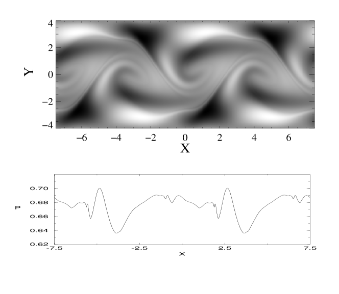
Abbildung 1: Phytoplankton smooth pattern in the closed flow, with an horizontal transect taken along $y=0.8$

*

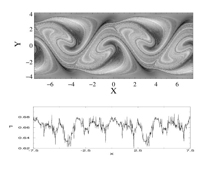
Abbildung 2: Phytoplankton filamental pattern in the closed flow, with a transect along $y=0.8$

5 Open flows

Contrarily to closed flows, open flows are characterized by unbounded trajectories of fluid particles. Typical fluid particles enter and, after some time, leave the region of the nutrient source ($C_{0}({\bf r})>0$). Thus, most fluid elements have only spent the most recent part of their trajectories inside the active region, with the rest of their evolution spent in regions with no spatial dependence of the nutrient input. For this part of the trajectory the gradient $\nabla f_{j}$ in Eq. (6) vanishes, implying that there would not be divergence of the gradients in the long-time limit.

It is well known from the study of chaotic advection in open flows (Péntek et al., 1995), that while most of the particles spend only a finite amount of time in selected bounded regions of the flow, typically these regions contain also bounded orbits in which some of the particles can stay forever. Although the chaotic set formed by the bounded orbits is a fractal set of measure zero, particles visiting the vicinity of the stable manifold of this set can still spend arbitrarily long time in the selected bounded region. This leads to the formation of characteristic fractal patterns in the advection dynamics even in the case of passive particles, as it was shown in numerical studies (Jung et al., 1993) and laboratory experiments of open flows (Sommerer et al., 1996).

For the particles that have spent infinitely long time in the source region, their chemical/biological evolution is equivalent to the one in a closed flow with the possibility of diverging gradients. The only difference is that now the values of $\lambda_{F}$ and $\lambda_{C}$ are those corresponding to the chaotic set of bounded orbits that never leave the biologically active region. The smooth-filamental transition observed in the previous Section for the closed flow will occur here only on this fractal set, which will always be surrounded by a smooth distribution. This results in a strongly intermittent character of the filamental field. Figure 3 shows a phytoplankton pattern for parameter values $\alpha=0.025,\delta=2.0$ and $A=0.2$, and a transect crossing it, in the open-flow case. The inhomogeneity in the filamental structure is obvious, with singularities in a set recognized as the unstable manifold of the chaotic set formed by bounded orbits in the source region. Smooth structures are also obtained when $\lambda_{F}+\lambda_{C}<0$. The proper description of the resulting structures should use the concept of multifractality, that is, inhomogeneous distribution of fractal properties. In fact, even in the closed flow case, at finite times the flow Lyapunov exponent $\lambda_{F}$ would have space-dependent finite-time corrections, that will need to be taken into account in a proper generalization of (6). A quantitative description of these multifractal filamental structures will be presented elsewhere (Neufeld et al., 1999b).

*

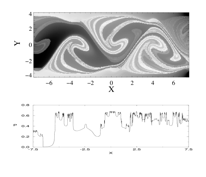
Abbildung 3: Phytoplankton filamental pattern in the open flow, with a transect along $y=0.8$.

6 Conclusions

The spatial patterns formed by interacting populations under the influence of chaotic flows have been studied. In particular, we have considered a coupled model of ‘nutrient’, phytoplankton and zooplankton concentrations advected by two (open and closed) jet-like flows. General results have been reported for arbitrary chaotic flows, stressing the existence of a smooth-filamental transition depending on the relative strength of the maximum Lyapunov exponent of the flow and the one corresponding to the planktonic dynamical system. Patterns obtained for open and closed chaotic flows are different because of the transient or permanent character of the biological activity. Comparison of the structures for the different fields (capacity, phytoplankton and zooplankton), and quantitative description of their multifractal properties will be presented elsewhere (Neufeld et al., 1999b).

The models considered here are extreme simplifications of real biological and geophysical situations. We expect however that the main qualitative features found here, namely the possibility of finding smooth or filamental patterns depending on stirring and relaxation rates, and the increased inhomogeneities in open flows, to be present in more realistic chemical or biological transport situations.