Numerical accuracy of Bogomolny’s semiclassical quantization scheme in quantum billiards

Abstract

We use the semiclassical quantization scheme of Bogomolny to calculate eigenvalues of the Limaçon quantum billiard corresponding to a conformal map of the circle billiard. We use the entire billiard boundary as the chosen surface of section (SOS) and use a finite approximation for the transfer operator in coordinate space. Computation of the eigenvalues of this matrix combined with a quantization condition, determines a set of semiclassical eigenvalues which are compared with those obtained by solving the Schrödinger equation. The classical dynamics of this billiard system undergoes a smooth transition from integrable (circle) to completely chaotic motion, thus providing a test of Bogomolny’s semiclassical method in coordinate space in terms of the morphology of the wavefunction. We analyze the results for billiards which exhibit both soft and hard chaos.

I Introduction

This paper presents a numerical investigation of Bogomolny’s semiclassical scheme for solving the quantum problem of a non-integrable billiard system. We deal with a single particle in a zero field environment making specular collisions with a closed and singly-connected boundary. The analogous quantum problem refers to the solution of the Helmholtz equation in a closed region B,

$$\Delta_{\vec{r}}\psi(\vec{r})+k^{2}\psi(\vec{r})=0$$ (1)

with Dirichlet boundary condition, $\psi(\vec{r})|_{\partial B}=0$ and $\hbar=1$, $2m=1$. Such a system is called a quantum billiard.

During the past twenty years a tremendous effort has been devoted to the study of quantum systems whose classical counterpart is chaotic. A detailed analysis of the results comprises the statistical properties of the energy spectrum and the geometric structure or morphology of the eigenfunctions and their statistics. Some recent reviews with many references to the progress made can be found in Gutzwiller’s book [1], Giannoni et al. [2] and Casati and Chirikov [3]. At the heart of these studies lies the issue of quantum chaos or the influence of classical chaos on the solutions of Eq. (1). On the one hand, past research has considered the statistics of the energy-level spectrum and has demonstrated the existence of universal classes for particular classical regimes. Integrable dynamics lead to uncorrelated energy levels (Poisson spectrum) and completely chaotic systems lead to Wigner-Dyson statistics of one of the standard ensembles of random matrices. On the other hand the notion of scars has played an important role in the study of eigenfunction structure [4, 5, 6, 7, 8, 9, 10].

As for the methods to solve the quantum problem, many have been proposed and the most successful will be quickly mentioned. Most textbooks deal with integrable systems since an analytic solution for the energy exists and can be easily written down. Unfortunately, they do not even mention generic non-integrable chaotic classical systems for which the quantum problem can only be solved numerically. Of all the methods, two have stood out to be particularly successful; they are the plane wave decomposition method (PWDM) invented by Heller[4, 11] and improved by Li et al.[8, 9, 12], and the boundary integral method (BIM) [13, 14, 15].

Other methods also deserve mention. Firstly we consider the conformal map diagonalization technique, which was first used by Robnik to calculate the eigenvalues of the Limaçon billiard [16]. This method makes use of a conformal map which transforms the boundary to an integrable geometry but adds additional terms to the Hamiltonian. This method was later invoked by Berry and Robnik[17], Prosen and Robnik [18] and Bohigas et al.[19]. In addition, the scattering quantization method introduced by Smilansky and co-workers [20] provides an alternative approach for solving the eigenvalue problem. Prosen [21] has extended this scattering quantization method to an exact quantization on the surface of section. In his method, the exact unitary quantum Poincaré mapping is constructed quite generally from the scattering operators of the related scattering problem whose semi-classical approximation gives exactly Bogomolny’s transfer operator which shall be studied exclusively in this paper. As for the method of calculating high-lying eigenstates, we would like to mention the method introduced by Vergini and Saraceno[22]. This method overcomes the disadvantage of missing levels via the PWDM and in the BIM, and can directly give all eigenvalues in a narrow energy range by solving a generalized eigenvalue problem. However, it is still not clear whether this method applies to a billiard having nonconvex boundary.

The above methods attempt to find solutions of the Schrödinger equation by an exact albeit numerical method and as a result a small error must be expected. Another approach, not exact, refers to quantization in the semiclassical limit, $\hbar\to 0$, or quantization of high lying eigenvalues. The study of quantum chaos and the extraction of eigenvalues via semiclassical methods began with the quantization of integrable systems or EBK theory. In the past forty years, though, much effort has been spent to extend the semiclassical approach to quantum systems whose classical counterpart is not integrable. Naturally, this study is intimately tied to the study of quantum chaos.

The first semiclassical approximations for classically chaotic systems are all based on the Gutzwiller trace formula (GTF) [1]. In this theory, the density of state ($\rho(E)=\sum_{i}\delta(E-E_{i})$) is expressed as a sum of two terms, the first being the usual Weyl formula or Thomas-Fermi density of states and the second being a long range surface correction term. In 2-D one writes:

$$\rho(E)\approx\bar{\rho}(E)+\Im m\frac{i}{\pi\hbar}\sum_{p}\sum_{r=1}^{\infty}\frac{T_{p}(E)}{\sqrt{|det(M^{r}_{p}(E)-I)|}}\exp{\left[(\frac{i}{\hbar}S_{p}(E)-i\frac{\pi}{2}\mu_{p})r\right]}$$ (2)

where the second term on the right hand side contains information pertaining to primitive periodic orbits and their repetitions, labeled by $p$. This includes the action $S_{p}$, the trace of the monodromy matrix $M^{r}_{p}$, a phase factor, $\mu_{p}$ and the geometrical period $T_{p}(E)=\frac{\partial S_{p}}{\partial E}$. While formally applicable for systems whose classical counterparts are either chaotic, integrable or a mixture of the two, the GTF (in its form written above) has been shown to fail, or at best proved difficult to implement for two independent reasons. One problem deals with mixed systems where the main contribution from bifurcating periodic orbits is divergent, $TrM_{p}\to\pm 2$, and has motivated a reevaluation of each orbit’s contribution close to the bifurcation. The other deals with the divergence of the sum due to an exponential proliferation of classical orbits (e.g. an exponential increase in the number of long-range periodic orbits with energy). In recent years, there have been many works devoted to overcome these two shortcomings of the GTF. On the one hand, the cycle expansion method [24] and an energy-smoothed version of the GTF [25] have been invented to provide a numerically efficient and convergent method to evaluate periodic-orbit expressions. On the other hand, many works have been down to the addition of higher terms of $\hbar$[26].

More recently another approach to the semiclassical quantization problem was presented by Bogomolny [27]. Bogomolny’s method makes use of a finite representation of a quantum Poincaré map in the semiclassical limit and leads to the calculation of a matrix whose eigenvalues allow one to determine an approximation to the true energy eigenvalues. It is founded on the BIM for determining wavefunctions inside a billiard system and its theoretical motivation came from two facts

• one, for generic billiard problems in any kind of external field, there does not exist an explicit closed form solution for the Green function;

• two, for general boundary condition involving $\psi$ and its derivatives one cannot reduce the solution of Eq. (1) to an integral equation which can be easily solved numerically as in typical problems where the BIM is useful.

Bogomolny worked around this by employing the standard semiclassical formula for the Green function in the energy representation and working in a boundary integral-like setting. He introduces by this way, a semiclassical transfer operator $T(E)$ and a quantization condition for an eigenvalue ${\bf det}(I-T(E))=0$.

Some past applications of Bogomolny’s method, include the following examples. It has been successfully applied to the rectangular billiard [29], and to billiards with circular symmetry [30, 31, 32]. All of these systems are integrable. For systems exhibiting hard chaos, we can mention applications to the geodesic flow on surfaces of constant negative curvature [33] and to the wedge billiard [34]. An interesting study [35] has also been carried out by applying Bogomolny’s transfer operator to a smooth nonscalable potential, the Nelson potential, at two fixed energies which correspond one to motion that is mostly integrable and the other mostly chaotic. However, to date an exhaustive test of the method for various classical regimes has not been done or at least not to very high energies. Goodings et al. [34] explore the first 30 eigenvalues for angles of the wedge billiard corresponding to soft chaos.

In this paper we report the results of Bogomolny’s semiclassical quantization scheme in a closed billiard whose boundary is derived from the quadratic conformal map of the unit circle [36], namely the Limaçon billiard. The mapping is controlled by a single parameter $\lambda$, with $\lambda=0$ corresponding to the circle billiard:

$$x = \cos(\theta)+\lambda\cos(2\theta)$$ (3)

$$y = \sin(\theta)+\lambda\sin(2\theta).$$ (4)

For all $\lambda,\;0\leq\lambda<1/4$ the boundary is analytic but non-convex for $\lambda>1/4$. The classical dynamics of this system has been extensively investigated[36], and shown to undergo a smooth transition from integrable motion, $\lambda=0$ to a soft chaos, KAM regime, $0<\lambda\leq 1/4$. At the convex-concave transition point, $\lambda=1/4$, the motion is very nearly ergodic [36]. While Hayli et al. [37] have shown that some very small stable islands still exist in the phase space, it can be supposed that above a $\lambda\approx 0.28$ these stable islands also disappear and the dynamics be that of hard chaos with mixing and positive K-entropy. A particular case is $\lambda=1/2$, for which the billiard boundary has one non-analytic point and it has been rigorously shown [38], that the motion exhibits hard chaos. For $\lambda=0.15$ the chaotic regions cover $64.6\%$ of the phase space and for $\lambda=0.2$ they cover more than $90\%$ [18].

To understand, at least, from a qualitative point of view, how Bogomolny’s semiclassical method might work in the Limaçon billiard we may consider three independent factors: (1) the success of the BIM without any semiclassical approximation; (2) the effects that a transition through a mixed regime will have on the morphology of each eigenstate; (3) the propensity of Bogomolny’s method for describing the energy of any particular kind of eigenstate based on the classification scheme, regular, mixed, and chaotic. The latter classification was first proposed by Percival [39] and used as the essential ingredients for the energy level statistics in mixed systems, namely the Berry-Robnik surmise [40]. Moreover, a detailed classification of states as being either regular or chaotic in the deep semiclassical limit has been performed with great success for the system studied here [41, 42] and also for much higher energy levels in another system[21]. However it is clear that this may not be possible at lower energies, the first 200 states, where the effective $\hbar$ occupies a phase space area $\propto 1/\sqrt{E}$ and is too large for sufficient resolution of projected states on a Poincare surface of section, (see Sec. 3). In this paper we will consider values of $\lambda$ corresponding to soft chaos, $\lambda=0.1,0.15$ and to harder chaos (or nearly hard chaos), $\lambda=0.2,0.23,0.245,0.25$. At $\lambda=0.15$ we also study the method in the deep semiclassical limit where a classification of states is possible.

As was stated above, the function, $det(I-T(E))$, equals zero as $E$ equals an energy eigenvalue. Most importantly, though, a formal relation between this determinant and the GTF has been demonstrated [27]

$$\ln\left({\bf det}(I-T^{osc}(E))\right)=\sum_{p}\frac{T_{p}}{\hbar\sqrt{|det(M_{p}-I)|}}\exp{\left(\frac{i}{\hbar}S_{p}-i\frac{\pi}{2}\mu_{p}\right)}$$

so that formally the zeros of the Bogomolny Transfer Operator $I-T(E)$ must be close to the positions of the poles of the GTF (the zeros of the former are separated from the poles of the latter by one stationary phase integral [27]). While strictly formal, this relation does beg a comparison between the two methods in the purely hard chaos regime and some very good results have been obtained using many thousands of unstable periodic orbits in strongly chaotic billiard systems [25]. But again, these results were obtained using methods that are most appropriate to systems exhibiting hard chaos and as such are not readily applicable to the system at hand.

II The transfer operator in coordinate space

We will deal with a closed billiard system with the Dirichlet boundary condition, in which the transfer operator of Bogomolny acts as a quantum Poincaré map [21]. We have mentioned that Bogomolny’s method is founded on the BIM. This interpretation however is not necessary. We may also derive Bogomolny’s quantization condition by starting with the general theory of quantum Poincaré maps (QPM). In this theory, one must initially define a certain surface of section (SOS), P, a set of coordinates $s$ on ${\it P}$ and a domain, ${\it L}$, for the QPM: in other words a set of ${\it L_{2}}$ functions in ${\it P}$.

Prosen [21] considers a certain non-unitary, compact QPM constructed from the product of two scattering transfer operators and shows that its semiclassical limit reduces to the transfer operator of Bogomolny. In general a QPM acts on $\psi_{1}\in{\it L}$ to give a $\psi_{2}\in{\it L}$. In the coordinates representation on ${\it P}$ this is given by,

$$\psi_{2}(s^{\prime})=\int_{SOS}dsT(s,s^{\prime},E)\psi_{1}(s)$$ (5)

A viable quantization condition (i.e. one that corresponds to the Schrödinger equation of the full system) can be obtained by requiring that for some energy, $E^{*}$, there exists some $\psi$ in L that is left unchanged after one Poincaré mapping [21]. This means that the QPM has at least one unit eigenvalue at $E^{*}$.

For generic problems one can construct a special scattering Hamiltonian in the SOS and from this an exact non-unitary compact QPM as in [20, 21]. On the other hand, to study the problem semiclassically one replaces the same QPM with its semiclassical limit which is Bogomolny’s transfer operator, $T^{osc}$ (from now on we denote the transfer operator of Bogomolny by $T^{osc}$ to distinguish it from any other QPM). Using Eq. (5), this leads to the familiar semiclassical quantization condition [27],

$${\bf det}(I-T^{osc}(E))=0$$ (6)

where $T^{osc}$ is constructed from classical trajectories passing from the SOS back to itself after one application of the QPM. The paper [21] also indicates how to treat higher order semiclassical errors for the energy (please also see [14, 26] and references therein).

In solving the equation (6) we must first express the transfer operator in a finite dimensional basis and the roots are then computed numerically. A particularly convenient choice for the SOS is the billiard boundary with a basis formed from a discretization of the boundary in either momentum or coordinate space. We have chosen the coordinate space representation and a discretization of the boundary into $N$ cells of length $\Delta_{m}(m=1,...,N)$. Let $s$ be the coordinate that measures distance along the boundary, and let $s=s_{n}$, $s^{\prime}=s_{m}$ be two points in two different cells. The semiclassical description for calculating the matrix element, $T^{osc}_{n\;m}$, is to sum over all possible classical trajectories which cross the SOS at $s_{n}$ and $s_{m}$ after one application of the Poincaré map,

$$T^{osc}(E)=\left\{\begin{array}[]{ll}\frac{-1}{(2i\pi\hbar)^{1/2}}|\frac{\partial^{2}S(s_{n},s_{m};E)}{\partial s\partial s^{\prime}}|^{1/2}\exp{\left[\frac{i}{\hbar}S(s_{n},s_{m};E)-i\frac{\pi}{2}\nu\right]}\sqrt{\delta_{n}\delta_{m}}&n\neq m\\ 1.0&n=m.\end{array}\right.$$ (7)

By using the entire boundary we have the numerical simplification that each cell is connected by one unique trajectory whose action $S(s_{n},s_{m};E)$ at energy $E$ is the length of the chord passing between these points multiplied by the factor $\sqrt{E}$. For the Dirichlet boundary condition and a convex geometry we put the phase index $\nu$ equal to 2 for all matrix elements. For the Dirichlet boundary condition and a non-convex geometry one can include ghost trajectories [27] that go outside the billiard to connect cells. Finally the prefactor in Eq. (7) contains the mixed second derivative of the action, $|\partial^{2}S/\partial s\partial s^{\prime}|^{1/2}$. The latter can be conveniently related to the linear Poincaré map for going from the boundary back to itself.

Bogomolny also writes down a prescription for the dimension of the transfer matrix which says that in passing from an operator to a finite representation one should give the $T$ matrix a dimension no smaller than the number given by:

$$dim(T)\geq{\it A}(E)/(2\pi\hbar)={\cal L}\sqrt{E}/\pi,$$ (8)

where ${\it A}$ is the classically allowed area, ${\cal L}$ is the billiard perimeter and $\hbar=1$. One could study the curve $f(E)={\bf det}(I-T^{osc}(E))$ but we prefer to examine individual eigenvalues of the $T$ matrix. In practice we do not exactly satisfy the quantization condition, only in the limit of an infinite transfer matrix can the unitarity condition of Bogomolny’s transfer operator be recovered and an eigenvalue of the matrix be exactly one. In this case we are obtaining an exact solution to Eq. (6).

Finally we note that the dimension of the $T^{osc}$ matrix is also equal to the number of cells on the SOS. Assuming that all cells have the same size we then define a parameter $b$, [14, 15], which represents the number of cells that make up one de Broglie wavelength, that is $b=2\pi dim(T)/(\sqrt{E}{\cal L})$. Or by using Eq. (8) this corresponds to $b$ being no smaller than two $2$ (at least $2$ cells per wavelength). Of course we should and must use a higher dimension and our calculations were performed with matrices exceeding the number in the Weyl formula for a one freedom by a factor of 10-20. In the very deep semiclassical limit, we were not able to go beyond $b\approx 5$ due to the limitation of computation facilities.

III Numerical calculation of eigenenergies

The boundary of the Limaçon billiard is given by Eq. (4). For $\lambda=0$ the eigenenergies are the zeros of the Bessel functions. Let us denote the $nth$ zero of the $mth$ order Bessel function by $\chi^{i}_{j}$. The quantum energies are given by the square of this for $\hbar=1$ and $m=0.5$. For $\lambda>0$ each zero $\chi^{i}_{j}(j>0)$ splits into an eigenstate of odd/even parity with respect to reflection on the x-axis. The $j=0$ order zeros, on the other hand, are associated with even states, so they do not satisfy the Dirichlet boundary condition on the x-axis.

In choosing an appropriate coordinate space basis, we have several choices:

• By choosing the entire billiard boundary as a basis and putting $\nu=2$ in Eq. (7) for all matrix elements we quantize implicitly all states which satisfy the Dirichlet condition for these values of $(x,y)$. Then since both odd and even states satisfy this condition, without any reference to the latter being zero also on the x-axis, we will obtain a spectrum for both symmetry classes.

• By choosing the upper boundary and x-axis as a basis and choosing $\nu=2$ for all matrix elements in Eq. (7) we will obtain a quantization for only odd states.

• By choosing a basis consisting of only half the boundary and constructing an appropriate symmetry desired Green function by placing a hard (resp. soft) wall on the x-axis we obtain a quantization condition for odd (resp. even) eigenvalues. In this case, however, we must include one or two trajectories going between each cell.

When the boundary is non-convex, $\lambda>0.25$, one must be careful in how to connect cells. In (i), certain pairs of cells cannot be connected. We then have the choice of putting that matrix element to zero or including the so-called ghost orbit [27]. In the latter case, however, not all matrix elements will have the same factor $\nu$. Noting that the matrix must be symmetric leads to the rule that the number $\nu$ is either zero or two depending on whether the trajectory crosses the SOS an even or odd number of times. For the purely convex case, $\lambda\leq 0.25$, all trajectoris cross the SOS only once after one Poincaré map and $\nu=2$. In (iii) we must decide which cells have one or two orbits connecting them; obviously if only a ghost orbit can connect two cells, there is only one trajectory, otherwise there are two trajectories. In order to compute only odd states, we can put a hard wall along the x-axis and consider a basis consisting of the x-axis and the upper boundary as in (ii). In (ii) one must consider only one trajectory connecting two cells. However, the odd state eigenvalues computed this way were found to be a factor of 10 worse than using choice (i) .

For $\lambda<0.25$ we find absolutely no contradiction with using (i) and all results presented in figures are based on this choice. Naturally we choose $\Delta_{i}=\Delta={\cal L}/dim(T)$ for all cells and from Eq. (4) we calculate the billiard’s area and perimeter. The latter, ${\cal L}$, is given by $4(1+2\lambda)E(8\lambda/(1+2\lambda))$ where $E(k)$ is the complete elliptic integral of the second kind. The half boundary perimeter plus the x-axis then has length, ${\cal L}_{1/2}=\frac{\cal L}{2}+2$. As for the billiard area ${\cal A}$, it is $\pi(1+2\lambda^{2})$. We then construct a formula for the number of odd and even states below some energy $E$, from the usual semiclassical formulae [18],

$$N_{odd}(E) = \frac{\cal A}{8\pi}E-\frac{{\cal L}_{1/2}}{4\pi}\sqrt{E}+\frac{5}{24}$$ (9)

$$N_{even}(E) = \frac{\cal A}{8\pi}E-\frac{{\cal L}-{\cal L}_{1/2}}{4\pi}\sqrt{E}-\frac{1}{24}.$$ (10)

Our quantum results were obtained from the conformal map diagonalization technique [18], and hereafter it is these values which are cited as the reference set of eigenvalues. These reference eigenvalues are calculated by using a very large Hamiltonian matrix (i.e. $dim=10000$) with the result that the lowest 1000 eigenvalues have an accuracy no worse than $10^{-10}$ of the mean level spacing. The numerical calculations for the transfer matrix and its roots were performed on a Compaq Alpha 2100. Often it was difficult to assign individual states to a semiclassical root at $\lambda=0.15$ and $\lambda=0.1$ where the level repulsion and the $y$ reflection symmetry were often not sufficiently broken. Moreover since our implementation of Bogomolny’s method is never more precise than $0.5$ percent of the mean level spacing it was an arbitrary choice in assigning to a pair of semiclassical roots an even and odd eigenvalue pair in the quantum spectrum separated by less than $0.1\%$ of the mean level spacing. Typically if two semiclassical eigenvalues are very close to two quantum eigenvalues, we assign one of the semiclassical eigenvalues to the quantum eigenvalue closest to it and the other semiclassical eigenvalue to the remaining quantum eigenvalue.

We show results for energies in the interval $E=(5,800)$ which includes approximately the first two hundred states ($\approx$ one hundred odd and one hundred even states) for the $\lambda$’s listed in the introduction. We also report results for an energy interval in the deep semiclassical limit for $\lambda=0.15$. We report all data in units of the mean level spacing such that if $E_{sc}$ is the semiclassically predicted eigenvalue and $E_{ex}$ is the quantum result, then the error we consider is

$$\alpha(E)=\log_{10}(|\Delta E|),\qquad\Delta E=N(E_{sc})-N(E_{ex})$$ (11)

In both Fig. (1) and Fig. (2) we plot $\alpha(E)$ as a function of $N(E_{ex})$.

In order to maintain consistently good precision the parameter $b$ must be kept constant over an entire energy range. On the other hand we consider a constant matrix dimension and span an appreciable energy range. So in the data of Fig (1) and Fig. (2) we use a matrix of size $350$ for all $\lambda$ in the energy interval $(5,800)$ and in this range $b$ decreases from $150$ to $10$, a considerable change. The error fluctuates between $-1.8$ and $-2.5$, with the mean $\approx-2.1$ (which means that the error is about one percent of the mean level spacing) but does not change appreciably even with the large change in $b$. Again we emphasize that the reference eigenvalues come from the matrix diagonalization technique. A rough mean obtained by using the BIM without any semiclassical approximation has been shown to be of order $10^{-4}$ or $0.01\%$ of the mean level spacing [15]. The semiclassical result obtained here is a factor of $100$ times less precise than the BIM if one uses $B\geq 10$. If one decreases $b$ to below ten, a deviation in accuracy does result and if one uses $b$ less than $3$, about $25\%$ of states in the spectrum are missed.

We present our results for $\lambda\geq 0.2$ in Fig (1). The results are equally good for both the softer chaos cases, $\lambda<0.2$ and shown in Fig. (2). From these figures and additional results performed at $\lambda=0.125,0.175,0.19$, it seems clear that there is no reason to believe that the Bogomolny method is better in one classical regime than in another. In Fig. (1) and Fig. (2) we see no deviation from a characteristic mean for any particular state, indicating that the method is unaffected by the classification of the wavefunction as being regular, chaotic or mixed. This is indeed unlike the result expected from the GTF; this semiclassical quantization tool would be invariably tedious to implement in the mixed regime. In the hard chaos regime, $\lambda=0.5$, and using a few short periodic orbits, the method has been shown to yield an accuracy of $8\%-10\%$ of the mean level spacing [44].

It must be pointed out that the slight increase of the semiclassical error with increasing sequence number in Fig. (1) and (2) is not due to the semiclassical method, instead it results from the decrease of $b$. Because in our numerical calculation, the dimension of matrix $dim(T)$ is fixed at 350 as aforementioned, thus $b\sim 1/\sqrt{N}$, where $N$ is the sequence number.

To verify the method for soft chaos at high energy, we explore a small energy range starting with the $10,603$rd even state with $dim(T)=1000$, and thus $b\approx 3.2$. The corresponding energy range, $E=(81435,81600)$ includes $24$ odd and 24 even states. At these energies a classification of each eigenstate in terms of a regular, chaotic or mixed description has been obtained but again our calculations confirm that Bogomolny’s scheme is independent of the eigenstate’s classification. We illustrate the $24$ even wavefunctions in coordinate space in Fig. (3) and as a smoothed Wigner function, see in Fig. (4). Their corresponding exact eigenenergy, the eigenenergy obtained by Bogomolmny’s scheme and their classification as being chaotic, regular, or mixed are presented in Table I. Compared with the average error at lower energy, one finds that the error is also slightly increased. Again, this is due to the decrease of $b$. This conclusion is different from that one obtained by Prosen and Robnik[18] for circular billiard with the torus quantization. There they found that the semiclassical quantization error increases with increasing energy.

The classification of eigenstates is based on the comparison of smoothed projective Wigner function and that of the classical as used in our previous work[41, 42]. The Wigner function (of an eigenstate $\psi(u,v)$) defined in the full phase space $(u,v,p_{x},p_{y})$ is

$$W({\bf q},{\bf p})=\frac{1}{(2\pi)^{2}}\int\;d{\bf X}^{2}\;\exp{(-i{\bf p}{\bf X})}\psi({\bf q}-\frac{\bf X}{2})\;\psi^{\dagger}({\bf q}+\frac{\bf X}{2})$$ (12)

Here $\psi$ is a function of two variables ${\bf q}=(x,y)$ and ${\bf p}=(p_{x},p_{y})$. We have also put $\hbar=1$. In order to compare the quantum Wigner functions with the classical Poincaré map we first choose a SOS (not the boundary) and define a projection of $W({\bf q},{\bf p})$ onto the SOS. The objective is to cast the Wigner function into a $2$-dim space of one coordinate and its conjugate momentum. We take the SOS to be the line $y=0$ and project the Wigner function of even states onto the $x-$axis,

$$\rho_{SOS}(x,p_{x},y=0)=\int\;dp_{y}\;W(x,y=0,p_{x},p_{y}),$$ (13)

which nicely reduces the number of integrations by one and is equal to

$$\rho_{SOS}(x,p_{x})=\frac{1}{2\pi}\;\int\;da\;\exp{(iap_{x})}\psi(x+\frac{a}{2},0)\psi^{\dagger}(x-\frac{a}{2},0).$$ (14)

As is well known that the Wigner function and its projections are not positive definite and indeed one typically finds small and inconvenient but nevertheless physical oscillations around zero which seriously obscure the main structural features. Therefore in order to compare the classical and quantal phase space structure we have smoothed the projection Eq. (14) by using a normalized Gaussian kernel with a suitably adapted dispersion, [45, 46].

In Fig. (3) we show the wavefunctions (in coordinate space) corresponding to $24$ eigenstates of even parity beginning with the $10,603$rd state. The reference eigenenergy was obtained by diagonalization of a $32000\times 32000$ matrix. In Fig. (4) we plot the smoothed object $\rho_{SOS}$ in Eq. (14). The lowest contour shown is at the level of $0.15$ of the maximal value and the step size upwards is $0.15$ of the maximum.

From a comparison of Fig. (4) and the classical phase space on the $y=0$ SOS in Fig. (5) we can classify the wavefunction as being either regular, chaotic or mixed. In Table I we note the classification and the precision of Bogomolny’s scheme. Again we hope that this small energy range, but nevertheless representative, can help to justify our conclusion that Bogomolny’s scheme is independent of the morphology of the eigenstate.

To examine the effect of increasing $b$ in the deep semiclassical limit, we consider the states 10610 (mixed), 10611 (chaotic) and 10612 (regular). The matrix dimension $dim(T^{osc})$ is increased from 700, 830 to 1000 which corresponds to the boundary node density $b$ is approximately changed from 2.45, 2.91 to 3.44, respectively. The results are shown in Table II. The enhancement of the accuracy is clearly shown in each of these three eigenstates of different classes.

As a further example, finally we consider the first hundred eigenstates of the Bunimovich stadium billiard with odd-odd parity. The dimensions are the following: the semicircle ends have radius $R=1$ and the half length of the straight segment $a$ is fixed at one. We consider both the quarter stadium with Dirichlet boundary conditions on all four walls and the entire boundary which will give all four symmetry classes. The classical dynamics of this system has been shown to be ergodic [43]. The quantum reference eigenvalues were computed by using the PWDM and are accurate to $10^{-4}$ of the mean level spacing[15]. A comparison of the semiclassical result and the reference eigenvalues, seen to be comparable with those obtained for the Limaçon billiard, are shown in Fig. (6).

IV Conclusion and discussions

We have studied the semiclassical quantization scheme of Bogomolny for two quantum billiard systems, one of which is classically ergodic for all physical parameters, the stadium billiard, and the other makes a smooth transition from integrability to hard chaos as a parameter $\lambda$ is changed.

We have studied the latter billiard for several values of $\lambda$ corresponding to both soft and hard chaos. We do not observe a dependence of the numerical accuracy of the method on the classification of the wavefunction as being either regular, chaotic or mixed. Furthermore with respect to a reference set of eigenvalues, the accuracy of the semiclassical method is on average about $1$ percent of the mean level spacing. Here we use the eigenvalues obtained by the matrix diagonalization technique as the reference set.

In the Bunimovich stadium billiard we obtain results for the first 100 states of odd-odd parity. We find that the method obtains results that are very much comparable with those for the Limaçon billiard.

As some further applications of this work we may consider the calculation of semiclassical eigenvalues in systems where ghost trajectories should be included in the calculation of the transfer matrix. Examples would include any billiard with a non-convex boundary (trajectories passing outside of the billiard) or billiards such as the Sinai and annulus billiard.

We could also consider an application of Bogomolny’s method in polygonal billiard systems with one angle a rational multiple of $\pi$, a so-called pseudo-integrable billiard [48, 49] where the wavefunction shows multifractality[50].

V Acknowlegements

We would like to thank Dr. Niall D. Whelan and Dr. Pei-Qing Tong for interesting discussions, and Dr. Toma$\check{z}$ Prosen for providing some of the reference eigenvalues of the Limaçon billiard. We are also very grateful to the anonymous referees for very useful comments and suggestions. This work was supported in part by the grants from the Hong Kong Research Grants Council (RGC) and the Hong Kong Baptist University Faculty Research Grants (FRG).

Table I. The classification of the 24 consecutive high-lying even states of the Limaçon billiard at $\lambda=0.15$. By comparing the smoothed function $\rho_{SOS}$ with the classical phase portrait (fig 5), we can distinguish the states as chaotic (C), regular (R) and mixed (M). The semiclassical eigenenergy obtained by Bogolmony’s scheme is given and compared with the reference quantum eigenenergies. The error is measured in the unit of the mean level spacing. For all these states we used a $1000$ dimensional array ($b\approx 3.51$) except for the $10,614,10,622$th and $10,623$th states. Here we had to use a larger matrix of dimension $1200$, ($b\approx 4.22$), since by using smaller $b$, these two levels are always missed. $N$ Classification $E_{ex}$ $E_{sc}$ $|\Delta E|$ 10603 c $81,361.69$ $81,361.88$ 2.4e-2 10604 c $81,369.91$ $81,370.10$ 2.4e-2 10605 c $81,372.41$ $81,372.51$ 1.3e-2 10606 c $81,377.38$ $81,377.52$ 1.8e-2 10607 c $81,382.99$ $81,382.77$ 2.8e-2 10608 c $81,398.52$ $81,398.39$ 1.6e-2 10609 c $81,408.35$ $81,408.50$ 1.9e-2 10610 m $81,435.34$ $81,435.57$ 2.9e-2 10611 c $81,441.86$ $81,442.05$ 2.4e-2 10612 r $81,451.87$ $81,452.47$ 7.5e-2 10613 r $81,455.08$ $81,455.35$ 3.4e-2 10614 c $81,458.73$ $81,459.03$ 3.8e-2 10615 r $81,462.10$ $81,462.28$ 2.3e-2 10616 m $81,472.86$ $81,472.97$ 1.4e-2 10617 c $81,501.51$ $81,501.76$ 3.1e-2 10618 c $81,504.34$ $81,504.65$ 3.9e-2 10619 r $81,507.96$ $81,508.23$ 3.9e-2 10620 c $81,511.94$ $81,512.05$ 1.4e-2 10621 c $81,512.74$ $81,512.95$ 2.6e-2 10622 c $81,534.52$ $81,535.00$ 6.0e-2 10623 r $81,536.83$ $81,537.03$ 2.5e-2 10624 c $81,538.91$ $81,539.09$ 2.3e-2 10625 r $81,543.85$ $81,544.07$ 2.8e-2 10626 c $81,558.03$ $81,888.24$ 2.6e-2

Table II. The dependence of the eigenenergies with the boundary nodes density $b$ for three different classes of eigenstates, regular, mixed and chaotic. The matrix dimension $dim(T^{osc})$ is increased from 700, 830 to 999. The boundary nodes density $b$ is approximately changed from 2.45, 2.91 to 3.44, respectively. The enhancement of the accuracy is demonstrated in each of these three eigenstates of different classes.

$N$	Classification	$E_{ex}$	$E_{sc}(b=2.45)$	$E_{sc}(b=2.91)$	$E_{sc}(b=3.44)$
10610	m	$81,435.34$	$81,435.68$	$81,435.62$	$81,435.58$
10611	c	$81,441.86$	$81,442.15$	$81,442.10$	$81,442.07$
10612	r	$81,451.87$	$81,452.52$	$81,452.50$	$81,452.47$

FIG. 1.: Results of Bogomolny’s transfer operator method for the hard chaos cases for both even (a,c,e) and odd (b,d,f) eigenstates. We draw $\alpha(E)=\log_{10}(|N(E_{sc})-N(E_{ex})|)$ versus $N(E_{ex})$. The top figures (a and b) are for $\lambda=0.2$, the middle figures (c and d) are for $\lambda=0.23$ and the bottom (e and f) are for $\lambda=0.245$. All results are with dim(T)=350. The lines are drawn for guiding the eye.

FIG. 2.: The same as Fig. (1) but for for $\lambda=0.1$ (a and b) and $\lambda=0.15$ (c and d). Again a and c are for even states, b and d for odd states. All results are for dim(T)=350. The lines are drawn for guiding the eye.

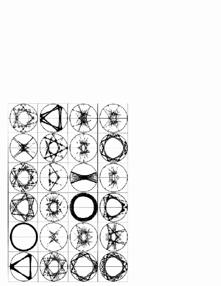
FIG. 3.: The gallery of wavefunctions in coordinate space for 24 consecutive eigenstates starting from the $10,603$rd state. The order is left-right and top-down.

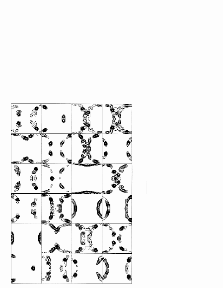
FIG. 4.: Smoothed object $\rho_{SOS}$ of the wavefunctions in Fig. (3). Again the order is left-right and top-down. The abscissa is from $-1+\lambda$ to $1+\lambda$, and the vertical axis from $-\sqrt{E}$ to $\sqrt{E}$. So the minimum quantum cell is about the size $4/\sqrt{E}$.

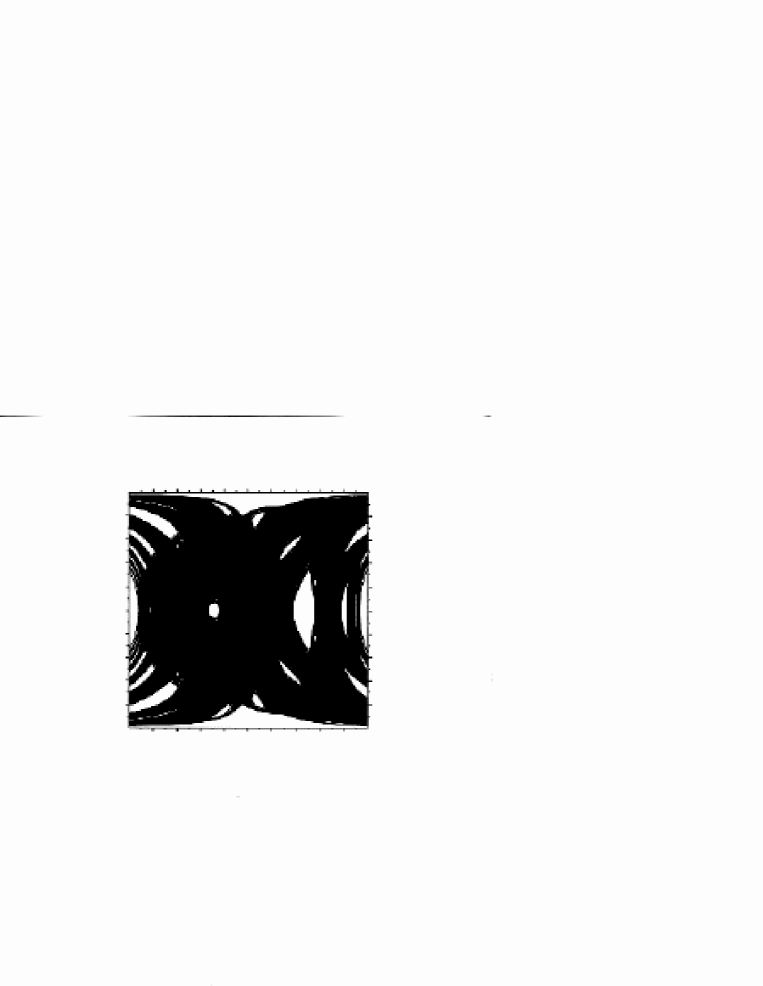
FIG. 5.: Portraits of the classical phase space on the $y=0$ for $\lambda=0.15$.

FIG. 6.: Results of Bogomolny’s transfer operator method for the odd-odd parity eigenstates in the stadium billiard. The top figure (a) refers to data using the quarter stadium and the lower figure (b) to the data using the whole stadium and extracting only those energies close to the reference eigenvalues. The lines are drawn for guiding the eye.

REFERENCES

- [1] M. C. Gutzwiller, Chaos in Classical and Quantum Mechanics, (New York: Springer 1990).
- [2] Chaos and Quantum Systems (Proc.NATO ASI Les Houches Summer School), ed. M-J Giannoni, A. Voros and J. Zinn-Justin (ed. Amsterdam: Elseivier), pg. 87.
- [3] G. Casati and B. V. Chirikov, Quantum Chaos, (Cambridge University Press, Cambdridge 1995).
- [4] E. J. Heller, Phys. Rev. Lett. 53, 1515 (1984).
- [5] E. B. Bogomolny, Physica D31 , 169 (1988).
- [6] M. V. Berry, Proc. R. Soc. A 423, 219 (1989).
- [7] O. Agam and S. Fishman, J. Phys. A 26, 2113 (1994); Phys. Rev. Lett. 73, 806(1994)
- [8] B. Li, Phys. Rev. E 55, 5376 (1997).
- [9] B. Li and B. Hu, J. Phys. A 31, 483 (1998).
- [10] L. Kaplan and E. J. Heller, Ann. Phys. (NY) 264, 171 (1998).
- [11] E. J. Heller, in Ref.[2], p. 548.
- [12] B. Li and M. Robnik, J. Phys. A 27, 5509 (1994).
- [13] M. V. Berry and M. Wilkinson, Proc. R. Soc. London A 392, 15 (1984).
- [14] P. A. Boasman, Nonlinearity 7, 5509 (1994).
- [15] B. Li, M. Robnik, and B. Hu, Phys. Rev. E. 57, 4095 (1998).
- [16] M. Robnik, J. Phys. A 17, 1049 (1984).
- [17] M. V. Berry and M. Robnik, J. Phys. A 19, 649 (1986).
- [18] T. Prosen and M. Robnik, J. Phys. A 26, 2371 (1993); ibid. 27, 8059 (1994).
- [19] O. Bohigas, D.Boosé, R. Egydio de Carvalho, and V. Marvulle, Nucl. Phys. A 560, 197 (1993).
- [20] E. Doron and U. Smilansky, Nonlinearity, 5, 1055 (1992); H. Schanz and U. Smilansky, Chaos, Fractals and Solitons 5, 1289 (1995).
- [21] T. Prosen, J. Phys. A, 27, L709 (1994); 28, L349, 4133 (1995); Physica D91, 244 (1996).
- [22] E. Vergini and M. Saraceno, Phys. Rev. E 52, 2204 (1995).
- [23] M. V. Berry and J. P. Keating, Proc. R. Soc. London A437, 151 (1992).
- [24] P. Cvitanović, Phys. Rev. Lett., 61, 2729 (1988); R. Artuso, E. Aurell, and P. Cvitanović, Nonlinearity 3, 325, 361 (1990).
- [25] R. Aurich, C. Matthies, M. Sieber, and F. Steiner, Phys. Rev. Lett. 68, 1629 (1992).
- [26] A M O de Almeida and J H Hannay, J. Phys. A, 20, 5873 (1987); P. Gaspard and D. Alonso, Phys. Rev. A 47, R3468 (1993); G. Vattay and P. E. Rosenqvist, Phys. Rev. Lett. 76, 335 (1996); G. Vattay, ibid. 76, 1059 (1996); H. Schomerus and M. Sieber, J. Phys. A, 30, 4537 (1997).
- [27] E. B. Bogomolny, Nonlinearity 5, 805 (1992).
- [28] P. Cvitanović and G. Vattay, Phys. Rev. Lett. 71, 4138 (1993); P. Cvitanović et al., Chaos 3 (4), 619 (1993); B. Georgeot and R. E. Prange, Phys. Rev. Lett. 74, 2851, 4110 (1995).
- [29] B. Lauritzen, Chaos 2, 409 (1992).
- [30] P. Tong and D. Goodings, J. Phys. A 29, 4065 (1997).
- [31] N. C. Snaith and D. A. Goodings, Phys. Rev. E 55, 5212 (1997).
- [32] D. A. Goodings and N. D. Whelan J. Phys. A 31, 7521(1998).
- [33] E. B. Bogomolny and M. Caroli, Physica D67, 88 (1993).
- [34] T. Szeredi, J. Levebvre and D. A. Goodings, Nonlinearity 7, 1463 (1994); Phys. Rev. Lett. 71, 2891 (1993).
- [35] M. R. Haggerty, Phys. Rev. E 52, 389 (1995).
- [36] M. Robnik, J. Phys. A 16, 3971 (1983).
- [37] A. Hayli, T. Dumont, J. Moulin-ollagier, and J. M. Strelcyn, J. Phys. A 20, 3237 (1987).
- [38] R. Markarian, Nonlinearity 6, 819 (1993).
- [39] I. C. Percival, J. Phys. B 6, L229 (1973).
- [40] M. V. Berry and M. Robnik, J. Phys. A 17, 2413 (1984).
- [41] B. Li and M. Robnik, J. Phys. A 28, 2799 (1995); B. Li and M. Robnik, chaos-dyn/9501022.
- [42] B. Li and M. Robnik, J. Phys. A 28, 4843 (1995).
- [43] L. A. Bunimovich, Funct. Anal. Appl. 8, 254(1974); Commun. Math. Phys. 65, 295(1979).
- [44] H. Bruus and N. D. Whelan, Nonlinearity 9, 1023 (1996) .
- [45] K. Takahashi, Prog. Theor. Phys. Suppl. 98, 109 (1989).
- [46] P. Leboeuf and M. Saraceno, J. Phys. A 23, 1745 (1990).
- [47] M. V. Berry, J. Phys. A 10, 2083 (1977).
- [48] P. J. Richens and M. V. Berry, Physica D 2, 495 (1981).
- [49] E. B. Bogomolny, U. Gerland and C. Schmit, Phys. Rev. E 59, R1315 (1999).
- [50] E. B. Bogomolny, Private communication.