The accurate and comprehensive model of thin fluid flows with inertia on curved substrates
Abstract
Consider the 3D flow of a viscous Newtonian fluid upon a curved 2D substrate when the fluid film is thin as occurs in many draining, coating and biological flows. We derive a comprehensive model of the dynamics of the film, the model being expressed in terms of the film thickness and the average lateral velocity . Based upon centre manifold theory, we are assured that the model accurately includes the effects of the curvature of substrate, gravitational body force, fluid inertia and dissipation. The model may be used to resolve wave-like phenomena in the dynamics of viscous fluid flows over arbitrarily curved substrates such as cylinders, tubes and spheres. We briefly illustrate its use in simulating drop formation on cylindrical fibres, wave transitions, Faraday waves, viscous hydraulic jumps, and flow vortices in a compound channel. These models are the most complete models for thin film flow of a Newtonian fluid; many other thin film models can be obtained by different truncations of the dynamical equations given herein.
1 Introduction
Mathematical models and numerical simulations for the flow of a thin film of fluid have important applications in industrial and natural processes [37, 35, 38, 39, 7, 12, 23, 10]. The dynamics of a thin fluid film spreading or retracting from the surface of a supporting liquid or solid substrate has long been active areas of research because of its impact on many technological fields, for example, coating flows [37]: applications of coating flows range from a single decorative layer on packaging, to multiple layer coatings on photographic film; coated products include adhesive tape, surgical dressings, magnetic and optical recording media, lithographic plates paper and fabrics. A wide variety of thin fluid film models have been reviewed in detail by Oron et al. [24]. In this Introduction, we summarise some of the results on mathematical models for three dimensional thin fluid film flows on a solid curved substrate and relate these to the new model derived herein.
In a three dimensional and very slow flow, a “lubrication” model for the evolution of the thickness of a film on a general curved substrate was shown by Roy et al. [36] to be
| (1) |
where is proportional to the amount of fluid locally “above” a small patch of the substrate; is the mean curvature of the free surface of the film due to both substrate and fluid thickness variations (); is the curvature tensor of the substrate; , and are the principal curvatures and the mean curvature of the substrate respectively (positive curvature is concave); is a Weber number characterising the strength of surface tension; and the differential operator is defined in a coordinate system on the curved substrate. Based upon a systematic analysis of the continuity and Navier-Stokes equations for a Newtonian fluid, this model accounts for any general curvature of the substrate and that of the surface of the film. Decré and Baret [10] found good agreement between a linearised version of lubrication models such as (1) and experiments of flow over various shaped depressions in the substrate.
In many applications the lubrication model (1) of slow flow of a thin fluid film has limited usefulness; instead a model expressed in terms of both the fluid layer thickness and an overall lateral velocity or momentum flux is needed to resolve faster wave-like dynamics in falling films [7, p110], wave transitions [8], higher Reynolds number flows [27, Eqn.(19)], in rising film flow and a slot coater [17, Eqn.(37)], and in general flows [14, 34]. Roberts [34] derived such a model for two dimensional flow, approximately
| (2) | |||||
| (3) |
where is a Reynolds number of the flow, is the lateral velocity averaged over the fluid thickness, and is the lateral component of gravity. Here we greatly extend the model (2–3) by deriving in §5 the approximate model for the flow of a three dimensional thin liquid layer of an incompressible, Newtonian fluid over an arbitrary solid, stationary and curved substrate, such as the flow about a cylinder shown in Figures 1 and 2.
 |
 |
 |
 |
 |
 |
 |
 |
The derived accurate model (52–53) for the film thickness and a weighted average lateral velocity , see (43), is to low order and analogous to (2–3)111The approximate equality in the conservation of mass equation (4) becomes exact equality when replaces on the left-hand side. The higher order analysis leading to (52) does this automatically.
| (4) | |||||
| (5) |
where is the component of gravity tangential to the substrate. The conservation of fluid equation (4) is the natural generalisation of equation (2) to three dimensional flow. The momentum equation (5) similarly generalises (3) to three dimensional flow through a nontrivial effect of curvature upon drag. The important feature of this model, as in (2–3), is the incorporation of the dynamics of the inertia of the fluid, represented here by the leading order term , which enables the model to resolve wave-like behaviour. In contrast, the lubrication model of thin films (1) only encompasses a much more restricted range of dynamics. We base the derivation of model (4–5) upon a centre manifold approach established in §4. The approach is founded on viscosity damping all the lateral shear modes of the thin fluid film except the shear mode of slowest decay. Then all the physical interactions between spatial varying quantities, substrate curvature, surface tension and gravitational forcing are systematically incorporated into the modelling because the centre manifold is made up of the slowly evolving solutions of the Navier-Stokes and continuity equations; for example, all these physical effects take part in the particular simulation shown in Figures 1 and 2. For example, the coefficient in the models such as (3,5) is not : the coefficient of these terms would be in modelling based upon the heuristic of cross sectional averaging; but is correct because it must be of the viscous decay rate in order to match the leading coefficient in the lubrication model (1). In this approach the model is based upon actual solutions of the Navier-Stokes equations and so gets all coefficients correct to a controlable order of accuracy.
Before we undertake the construction we introduce in §2 an orthogonal curvilinear coordinate system fitted to the substrate. The analysis then starts from the incompressible Navier-Stokes equations and boundary conditions recorded in §3 for this special coordinate system. Thus we derive the model for a completely general curving substrate.
The derived model (52–53) reduces to a model for three dimensional fluid flow on flat substrates upon setting the principle curvatures and equal to zero. For example, the low order model (5) becomes simply
| (6) |
The higher order accurate version of this model, recorded in §6.1 as (59–61), extends to three dimensional fluid flows the models for two-dimensional fluids on flat substrates that were derived in [34, 14]. In §6.1 we report on the linearised dynamics, where both and are small. One result is that
| (7) |
where is a measure of the mean vorticity normal to the substrate in the flow of the film. Thus mean normal vorticity just dissipates due to drag and diffusion. However, letting , which measures the mean divergence of the flow of the film and hence indicates whether the film is thinning or thickening, we find
| (8) | |||||
| (9) |
where . Observe that this divergence diffuses with a larger coefficient, namely , than that of pure molecular diffusion; this effect is analogous to the enhanced Trouton viscosity of deforming viscous sheets [28, p143, e.g.]. The enhanced viscous dissipation is due to interactions with the shear flow similar to those giving rise to enhanced dispersion of a passive tracer in pipes [21, e.g.]. From (9) see that the divergence of the film’s velocity is simply driven by gravity and surface tension acting on variations of the film’s thickness and is dissipated by substrate drag and the enhanced lateral diffusion. Nonlinearities and substrate curvature modify this simple picture of the dynamics.
Circular cylinders are a specific substrate of wide interest. For example, Jensen [15] studied the effects of surface tension on a thin liquid layer lining the interior of a cylindrical tube and derived a corresponding evolution equation. Whereas Atherton & Homsy [2], Kalliadasis & Chang [16] and Kliakhandler et al. [18] considered coating films flow down vertical fibres and gave nonlinear lubrication models. Thus in §6.2 we also record the accurate model for flow both inside and outside a cylinder as used in the simulations for Figures 1 and 2. Axisymmetric flows are often of interest in coating flows. Using as the axial coordinate, to low order a model for axisymmetric film flow along a cylinder of radius is
| (10) | |||
| (11) |
where the upper/lower sign corresponds to flow on the outside/inside surfaces of the cylinder. Observe that the curvature of the substrate: modifies the expression of conservation of mass; drives a beading effect through ; and modifies the drag terms. These are just some special cases of those recorded in §6.
The centre manifold approach we use to derive low-dimensional dynamical models such as (4–5) has the advantage that its simple geometric picture leads to a complete low-dimensional model [21, e.g.]. Algebraic techniques have been developed for the derivation of a low-dimensional model [33], the correct modelling of initial conditions [9, 30, 40] and boundary conditions [31]. However, we limit our attention to deriving the basic differential equations of the dynamical flow. Other aspects of modelling remain for further study. But further, at the end of §5 we investigate high order refinements of the basic linearised surface tension driven dynamics of (7–9) and determine that the model (52–53) derived here requires that spatial gradients are significantly less than the limit , for example, see (57). This quantitative indication of the extent of the model’s spatial resolution is better than that for lubrication models such as (1) which require the surface slope to be significantly less than instead. Such quantitative estimates of the range of applicability are found through the systematic nature of the centre manifold approach to modelling.
2 The orthogonal curvilinear coordinate system
In this section, we describe the general differential geometry necessary to consider flows in general non-Cartesian geometries. First, we introduce the geometry on the substrate, then extend it out into space and establish the orthogonal curvilinear coordinate system used to describe the fluid flow.
Let denote the solid substrate. When has no umbilical point, that is, there is no point on at which the two principal curvatures coincide, then there are exactly two mutually orthogonal principal directions in the tangent plane at every point in [13, Theorem 10-3]. Let and be the unit vectors in these principal directions, and the unit normal to the substrate to the side of the fluid so that , and form a right-handed curvilinear orthonormal set of unit vectors. Such a coordinate system is called a Darboux frame [13]. Let and be two parameters such that the unit tangent vector of a parameter curve constant is , the unit tangent vector of a parameter curve =constant is , and let measure the normal distance from the substrate. Then on the substrate, points ,
| (12) |
with substrate scale factor
| (13) |
Further, we deduce how the normal varies along the substrate:
| (14) |
Note that the unit vectors are independent of . At any point in the fluid, written as
the scale factors of the spatial coordinate system are, since positive curvature corresponds to a concave coordinate curve,
The spatial derivatives of the curvilinear unit vectors are [3, p598]
where is the complementary index of and denotes .
A fundamental quantity for the problem is the free-surface mean curvature which is involved in the effects of surface tension through the energy stored in the free-surface. As derived by Roy et al. [36, eqn(37)], the mean curvature of the free-surface
where are the metric coefficients evaluated on the free surface (indicated by the tilde), and where
,
is proportional to the free-surface area above a patch of the substrate.
In the analysis we assume the film of fluid is thin. Conversely, viewing this on the scale of its thickness, the viscous fluid is of large horizontal extent on a slowly curving substrate. Thus we treat as small the spatial derivatives of the fluid flow and the curvatures of the substrate; Decré & Baret [10, p162] report experiments showing that apparently rapid changes in the substrate may be treated as slow variations in the mathematical model. Then an approximation to the curvature of the free surface is
| (15) |
where the Laplacian is evaluated in the substrate coordinate system as
| (16) |
For later use, also observe that on the free-surface the unit tangent vectors and unit normal vector are
| (17) |
| (18) |
We describe the dynamics of the fluid using these formula in a coordinate system determined by the substrate upon which the film flows.
3 Equations of motion and boundary conditions
Having developed the intrinsic geometry of general three dimensional surfaces, we proceed to record the Navier-Stokes equations and boundary conditions for a Newtonian fluid in this curvilinear coordinate system.
Consider the Navier-Stokes equations for an incompressible fluid flow moving with velocity field and with pressure field . The flow dynamics are driven by pressure gradients along the substrate which are caused by both surface tension forces, coefficient , the forces varying due to variations of the curvature of the free surface of the fluid, and a gravitational acceleration, , of magnitude in the direction of the unit vector . Then the continuity and Navier-Stokes equations are
| (19) |
| (20) |
We adopt a non-dimensionalisation based upon the characteristic thickness of the film , and some characteristic velocity : for a specific example, in a regime where surface tension drives a flow against viscous drag the characteristic velocity is and the Weber number . Reverting to the general case, the reference length is , the reference time , and the reference pressure . Then the non-dimensional fluid equations are
| (21) |
| (22) |
where is a Reynolds number characterising the importance of the inertial terms compared to viscous dissipation, and is a gravity number analogously measuring the importance of the gravitational body force compared to viscous dissipation; the gravity number for Froude number so that when we choose the reference velocity to be the shallow water wave speed then and the gravity number .
In the curvilinear coordinate system defined in §2 the non-dimensional continuity and Navier-Stokes equations for the velocity field are as follows (adapted from [3, p599]):
| (23) | |||
| (24) | |||
where is the vorticity of the fluid given by the curl
and where
These partial differential equations are solved with the following boundary conditions.
-
1.
The fluid does not slip along the stationary substrate, that is
(25) -
2.
The fluid satisfies the free surface kinematic boundary condition
(26) -
3.
The normal surface stress at the free surface is caused by surface tension, in non-dimensional form
(27) where is the deviatoric stress tensor on free surface, is the fluid pressure at the surface relative to the assumed zero pressure of the negligible medium above the fluid, and is the unit normal to the free surface.
-
4.
The free surface has zero tangential stress
(28) where is any tangent vector to the free surface. We use the two linearly independent tangent vectors in (17) to ensure the boundary condition is satisfied for all tangent vectors.
In this curvilinear coordinate system the components of the nondimensional deviatoric stress tensor are [3, p599]
| (29) | |||||
4 The centre manifold analysis of the dynamics
We adapt the governing fluid equations (23–24) and the four boundary conditions (25–28) to a form suitable for the application of centre manifold theory and techniques to generate a low-dimensional dynamical model with firm theoretical support.
Three mathematical tricks place the equations within the centre manifold framework; these tricks fit the parameter regime of viscous flow varying relatively slowly over the substrate.
-
1.
First we introduce the small parameter to characterise both the slow gradients along the substrate, , and the small curvatures of the substrate (as curvatures are the partial derivatives of unit normal with respect to ). either may be viewed at face value as a mathematical artifice or may be viewed as being equivalent to the multiple-scale assumption of variations occurring only on a large lateral length scale (large compared to the thickness of the fluid). The two viewpoints provide exactly the same results. In either case, let the lateral variations scale with the parameter :
where denotes quantities which have been scaled by .
-
2.
Second, the presumed small gravitational forcing is treated as a perturbing “nonlinear” effect by introducing the parameter such that the gravity number .
-
3.
Third, as introduced by Roberts [34], we also modify the tangential stress condition (28) on free surface, using a parameter : at the lateral shear mode of slowest decay actually becomes a marginally stable mode; whereas at the modification vanishes to restore the physical stress-free boundary condition (28). The modification to (34) is necessary to create the necessary three modes of the centre manifold model. Subsequently, evaluating at removes the modification to obtain a model for the physically correct dynamics.
Now rewrite the governing fluid equations according to the above tricks. For convenience, we drop the “” superscript on all re-scaled variables hereafter. Equations (23–24) become
| (31) | |||||
where the scale factors are , and the components of the vorticity are
The boundary conditions (25–28) become
| (32) |
| (33) |
| (34) |
| (35) |
where
and the unit tangent vectors and unit normal vector are
The asymptotic expressions for the deviatoric stress on the free surface are
| (36) | |||||
and the mean curvature of the free surface , expanded in powers of , is
where is the same as that in (16) and .
The tangential stress boundary condition (34) has been modified by the introduction of the artificial parameter . The physically correct boundary condition is recovered when . But when the boundary condition (34) linearises to
which gives two neutral horizontal shear modes, . The above equations have generalised the physical equations by introducing the extra parameters , and . Then by adjoining the trivial equations
| (37) |
we obtain a new dynamical system in the variables , , , , and . The original system will be recovered by setting , and . However, the two systems are quite different from the view of centre manifold theory. The theory now treats all terms that are multiplied by the three introduced parameters as nonlinear perturbing effects on the system. So the dynamics we describe will be suitable only when there are slow lateral variations in of the curvatures of the substrate, of , and , small , and a relatively weak gravitational forcing on the system, small . In §5 we argue that evaluating at is sound, and towards the end of §5 we give evidence that lateral variations are slow enough if their logarithmic derivative is less than . We now proceed to use centre manifold techniques to develop a model of the dynamics.
A linear picture of the dynamics is fundamental to the application of centre manifold techniques to derive a low-dimensional model. The linear part of system (31–31), that is omitting all terms multiplied by a small parameter , or , is
| (38) | |||||
| (39) |
with the boundary conditions (32–35) linearised to
| (40) | |||||
Note that there are no curvature nor lateral variations in the above linear equations, such variations are not included in the leading order approximation to the physical system. The linear dynamical system has three types of solutions: first, a motionless film of constant thickness , ; second, the family of lateral shear modes where
| (41) |
and third, the trivial , and being independently constant. Thus, the six modes corresponding to zero eigenvalues, the so-called critical modes, are the four modes with , , and arbitrarily constant, and the two modes with (obtained in the limit ). All other modes correspond to negative eigenvalues given by (41)—they are damped by viscosity. Consequently the centre manifold model which we create has six modes: three corresponding to critical physical modes; and three corresponding to trivial parameter modes.
Centre manifold techniques are justifiably applied to infinite dimensional dynamical systems whose linearisation has only non-positive eigenvalues and such that the nonlinear perturbation terms in the system are smooth and bounded, see Gallay [11]. The perturbation terms in system (31–31), involving spatial derivatives, are strictly speaking unbounded so the rigorous theory does not apply. Nonetheless, by restricting attention to slowly varying solutions only, the derivatives remain bounded and the resulting model is expected to be accurate [29]. With this proviso, a low-dimensional model of the system may be derived using centre manifold theory.
Denote the physical fields by . Centre manifold theory guarantees that there exist functions and of the critical modes where the critical modes evolve in time, that is
| (42) |
where there is implicit dependence upon the parameters , which are treated as small constants, and where are depth-averaged lateral velocities defined precisely as
| (43) |
This definition ensures that the fluid flux over a point on the substrate is simply . We proceed to find functions and such that as described by (42) are actual solutions of the physical equations (31–31) satisfying boundary conditions (32–35). We calculate and by an iteration using computer algebra [33], see Appendix A. In outline, suppose that an approximation and has been found, and let and denote corrections we seek to improve and . Substituting
into (31–31) and its boundary conditions then rearranging, dropping products of corrections, and using the linear approximation wherever factors multiply corrections (see [33] for more details), we obtain a system of linear equations for the corrections. The resulting system of equations is in the homological form
| (44) |
where is the linear operator on the left hand side of system (38–40), is a matrix, and is the residual of the governing equations (31–31) and boundary conditions (32–35) using the reigning approximations and . The procedure for solving the homological equation (44) is as follows: first, choose such that is in the range of ; second, solve making the solution satisfy the boundary conditions (32–35) and the definitions (43). Then regard and as the new approximation and respectively. Repeat the iteration until satisfied with the approximation. The ultimate purpose is to make the residual become zero to the required order of error, then the Approximation Theorem [6] in centre manifold theory assures us that the low-dimensional model has the same order of error. The computer algebra program listed in Appendix A performs the computations.
5 The high order model of film flow
The computer algebra program listed in Appendix A gives the physical fields of slowly varyingthin film fluid flow, and also describes the evolution thereon as a set of coupled partial differential equations for the evolution of the film thickness and the averaged lateral velocities .
Computing to low order in the small parameters, it gives the following fields in terms of the parameters and a scaled normal coordinate :
| (45) | |||||
| (46) | |||||
| (47) | |||||
where is the component of gravity in the direction normal to the substrate. The error terms in these expressions involve , and then is used to denote terms for which either is bounded as , or is bounded as . The corresponding evolution to this order of accuracy is
| (48) | |||||
| (49) | |||||
Throughout is the curvature tensor which in the special coordinate system chosen to fit the substrate takes the diagonal form
| (50) |
Although derived in the special coordinate system, the above and later results are all written in a coordinate free form. The differential operators that appear are those of the substrate. In the special orthogonal coordinate system they involve the substrate scale factors as in the Laplacian (16).
To recover the original model, we need to set so that (34) reverts to the physically correct boundary condition. In the above asymptotic expansions every coefficient is a series in , and the ratios of the coefficients of to in all such series appear to be greater than about for from further calculation. That is, the radii of convergence of the various series’ in are greater than about . Table 1 shows the coefficients of the series of some terms in a higher order version of the low-dimensional model (49). Evidently the convergence of at least these series’ is very good—we may expect five decimal place accuracy from the shown terms and similar for the other coefficients. A similar argument on the convergence of such series is reported in [34, 32].
Hence we justifiably substitute into the series of every coefficient to obtain the physical model. Here we generally calculate every coefficient in the evolution from the terms in the series up to and including those of order . We also now set to recover the unscaled model of the original dynamics. With higher order corrections in the low-dimensional model (49) then becomes the model (5) discussed briefly in the Introduction.
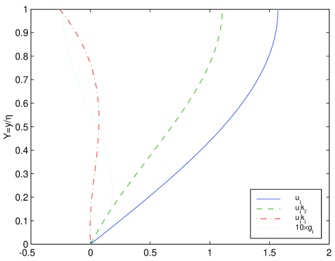
The low order expressions (45–47), when , give approximations to the physical state of the fluid flow corresponding to a given , and . Higher order expressions for the normal structure of the lateral velocity are plotted in Figure 3. The solid curve shows the fundamental structure of the lateral velocity in the normal direction; qualitatively it is dominantly parabolic, but it differs in detail. It is indistinguishable from the trigonometric expected from the correct linear problem [32], and thus is slightly faster at the free surface than the parabolic profile with the same flux. The dashed curve shows that in order to maintain the flux the flow along a trough, , has to be proportionally faster. The dot-dashed curve shows that flow curving upwards, around an internal corner, is slower at the free surface and conversely faster for flow around an external corner; part of this effect could be attributed to solid body rotation being the dissipation free mode for turning a corner. Lastly, the dotted curve, exaggerated by a factor of ten, shows the very small adjustment made to the profile when the flow is driven by gravity or lateral pressure gradients—observe the velocity at the free-surface will decrease slightly so that when lateral forces exactly balance the drag on the substrate the profile will be then the familiar parabolic Pouiseille flow. These show how just some of the physical processes affect the details of the physical fields and thus indirectly influence the evolution.
The shear stress on the substrate is of interest:
| (51) | |||||
The first term is just the viscous drag on a flat substrate. The next is the enhanced stress transmitted to the substrate when the fluid is driven by a body force or pressure gradients, equivalently. The third and last term accounts for the effects of curvature on the velocity field affecting the velocity profile near the bed.
Higher order model.
With computer algebra we readily compute a more accurate, more comprehensive higher order model. Atherton & Homsy [1] and Lange [19] have similarly considered high order models of thin film flows obtained via computer algebra but only in the lubrication approximation. Computing to the next order in spatial gradients , velocity field , and gravitational forcing , the model is written as follows:222Some of the constants that appear here are tentatively identified: , , and perhaps .
| (52) | |||||
| (53) | |||||
where the differential operators are those of the substrate coordinate system, noting in particular that [3, p599]
Observe that fluid is conserved by (52). In the above model (53) for the average velocity field we identify the apparent physical source of the terms in the various lines by the cryptic words to the left of the lines. Generally the viscous drag on the bed, surface tension forces and gravitational forcing show some subtle effects of the curvature of the substrate. In faster flows of higher Reynolds number, the most usually modelled part of the advection terms, the self-advection term , has the definite coefficient . But note that some of the self-advection is also encompassed within the term. This modelling settles, see for example [27, Eqn.(19)] or [26, Eqn.(23)], the correct theoretical value for this and other coefficients. The lateral damping via viscosity seems most natural to express in a mixed form involving both the general grad-div operator and the curl-curl operator (recall the vector identity ). The involvement of fractional powers of the film thickness within the scope of these operators is a convenient way to reduce the number of terms within the equation; as yet we have not discerned any interesting physical significance to this arrangement. You may truncate the above model in a variety of consistent ways depending upon the parameter regimes of the application you are considering.
Lubrication models
such as (1) may be derived from (52–53). Obtain simple low order accurate models simply by balancing the drag terms, dominantly , against the driving forces expressed by the surface tension and gravity terms. This then expresses the average velocity field as a function of the film thickness . This is substituted into the conservation of fluid equation (52) to form a lubrication model. Higher order, more sophisticated models are formed by then taking into account the consequent time dependence of the weaker previously neglected terms in (53). Any resultant lubrication model is correct because rational mathematical modelling is transitive: a coarser model of a model of some dynamics is the same as the coarser model derived directly.
Slower flow
occurs when in a specific application the velocity field is predominantly driven by surface tension acting because of curvature gradients, whence . The lateral velocities are significantly damped by viscous drag on the substrate. In this case truncate (53) to
| (54) | |||||
That is, you may adjust the dynamical model (53) to suit a particular application by choosing an appropriate consistent truncation.
Order one gradients are encompassed
by the model (53). ‘Long wave’ models such as (53) and (54) are based upon the assumption that the lateral spatial gradients are small. We here quantify what a ‘small gradient’ means in this context following similar arguments for the Taylor model of shear dispersion [20, 42]. We modify a simpler version of the computer algebra derivation of Appendix A to find the centre manifold model of the linear dynamics about a stationary constant thickness fluid with surface tension but no gravity: and where333The coefficients in the linear model (56) come from evaluating at an expansion with errors . The coefficients used here should be accurate as discussed earlier and demonstrated in Table 1.
| (55) | |||||
| (56) | |||||
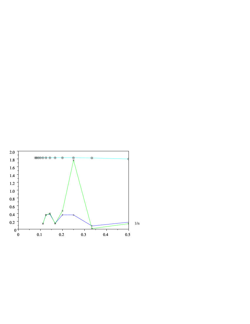
Evidently the linear dynamics are a formal expansion in . This expansion will converge when the lateral gradients are not too steep. Suppose locally a solution has spatial structure approximated by an exponential variation, say , then the above expansions become power series expansion in . The Domb-Sykes plot [20] of the ratio of successive coefficients in Figure 4 suggests that the power series converges for less than something roughly in the range to . The constant sign of the coefficients in (56) indicates the convergence limiting singularity occurs for real steep gradients. But the strong period 3 oscillations in the Domb-Sykes plot of the ratio indicates a complex conjugate pair of singularities occur at an angle of to the real axis at nearly the same ‘distance’. The generalisation of the Domb-Sykes plot to cater for multiple comparable limiting singularities [42] indicates that the three singularities are at a distance about ; that is, for any quantity , the magnitude of the logarithmic derivative of the lateral structure
| (57) |
for the model to converge. For example, apply this limit to the surface thickness, , to deduce that the steepness of the fluid variations , and that accurate approximation is achieved for steepnesses significantly less than this rough limit. Hence, steepnesses up to about one should be reasonably well represented by those low order terms appearing in the model (53).
For interest, we also investigated the analogous but poorer spatial resolution of the lubrication model (1) of thin film flow [36, e.g.]. The analogous high order but linear model is
| (58) | |||||
Continuing this expansion to errors see in its Domb-Sykes plot in Figure 4 that this power series converges only for much less rapid variations than the model (53). For example, the fluid thickness steepness , and so should be less than about a third, say, in order for the usual first term in the lubrication model to be reasonable. Thus expect the model (53) developed here to resolve spatial structure roughly three times as fine as a lubrication model.
6 The model on various specific substrates
The model (52–53) is quite sophisticated. It is not obvious how it will appear in any particular geometry. Thus in this section we record the model for four common substrate shapes: flat, cylindrical, channel and spherical. The models are given in terms of elementary derivatives rather than vector operators for easier use in specific problems.
6.1 Flow on a flat substrate resolves a radial hydraulic jump
The simplest example is the flow on a flat substrate. We: show 1D wave transitions; simulate Faraday waves; explore divergence and vorticity in the linearised dynamics; and lastly demonstrate that modelling the inertia enables us to resolve hydraulic jumps in a radial flow.
On a flat substrate use a Cartesian coordinate system and let the mean lateral velocity have components and respectively (note that in this subsection is a tangential coordinate, not a normal coordinate). The substrate has scale factors , and curvatures . The model (52–53) becomes, where is the direction cosine of gravity normal to the substrate into the fluid layer and where subscripts on denote partial derivatives,
| (59) | |||||
| (60) | |||||
| (61) | |||||
Observe that the substrate drag, gravitational and surface tension terms are quite straightforward. However, the self-advection terms exhibit subtle interactions between the components of the velocity fields due to the specific shape of the velocity profiles. Further subtleties occur in the viscous terms which not only show explicitly a differential lateral dispersion of momentum, but also a complex interaction with variations in the free surface shape.
Wave transitions:
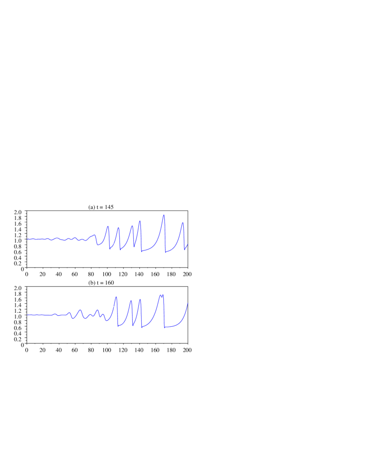
this model resolves 1D wave transitions such as those reported by Chang, Demekhin and Saprikin [8]. Their parabolicised Navier-Stokes equation (1) corresponds to our non-dimensional Navier-Stokes equation (22) with and our Reynolds number for Chang et al’s . See the corresponding simulations of our model (59–60) restricted to 2D flow (as in [32]) and forced by white noise at the inlet, although the forcing here is a little larger than that of Chang et al. [8]: the evolution and merger of the solitary pulses are qualitatively the same as that simulated by Chang et al. The only noticeable difference is that the retained dissipation in our modelling almost entirely removes the surface tension waves in front of the solitary pulses.
 |
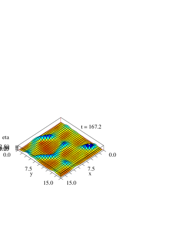 |
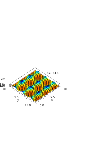
Faraday waves
Vigorous vertical vibration of a layer of fluid on a flat plate leads to a rich repertoire of spatio-temporal dynamics [22, 25, e.g.], such as those shown in Figure 6. We choose the reference velocity to be the shallow water wave speed then the non-dimensional parameters . Achieve the vertical vibration simply by modulating the normal gravity in (60–61) by, for example, the factor . This frequency is roughly twice that of waves with wavelength and see in Figure 6 that these waves are generated by a Mathieu-like instability. But involved nonlinear interactions lead to complex evolution of the spatial pattern of waves.
Vorticity and divergence
We explore some more of the dynamics described by the model (59–61). Consider the linearised dynamics of small variations on a film of nearly constant thickness: where and the lateral velocity are small. The linearised versions of (59–61) are:
where (the name is chosen because its value is coincidentally close to ).
-
•
First take of the second from of the third to deduce equation (7) governing the mean normal vorticity . Observe that linearly it is decoupled from the other components of the fluid dynamics: the mean normal vorticity simply decays by drag on the substrate and by lateral diffusion.
-
•
Conversely, the first of the linearised equations together with the divergence of the second two equations decouple from the mean normal vorticity to give (8–9) for the film thickness and the mean flow divergence as discussed briefly in the Introduction. A little analysis shows that in the absence of gravity () this model predicts damped waves for lateral wavenumbers
Numerical solutions of the physical eigenvalue problem agree closely with this for even though the critical wavenumber is as large as . Recall that the limit (57) on logarithmic derivatives in this model implies the wavenumber must be less than ; here the critical on a fluid of depth near is comfortably within the limit. Waves cannot be captured by the single mode of a lubrication model such as (1).
-
•
Lastly, in this linear approximation, lateral components of gravity just induce a mean flow in the direction of the lateral component.
Substrate curvature and the nonlinear effects of advection and large-scale variations in the thickness modify this description of the basic dynamics of the fluid film.
Radial flow with axisymmetry:
turn on a tap producing a steady stream into a basin with a flat bottom: you will see the flow spreads out in a thin layer, then at some radial distance it undergoes a hydraulic jump to a thicker layer spreading more slowly [41, e.g.]. A model with inertia is essential for modelling such a hydraulic jump. Here use polar coordinates , whence the substrate has zero curvature , but scale factors and . Then describe axisymmetric dynamics by neglecting angular flow and variations while retaining the radial velocity :
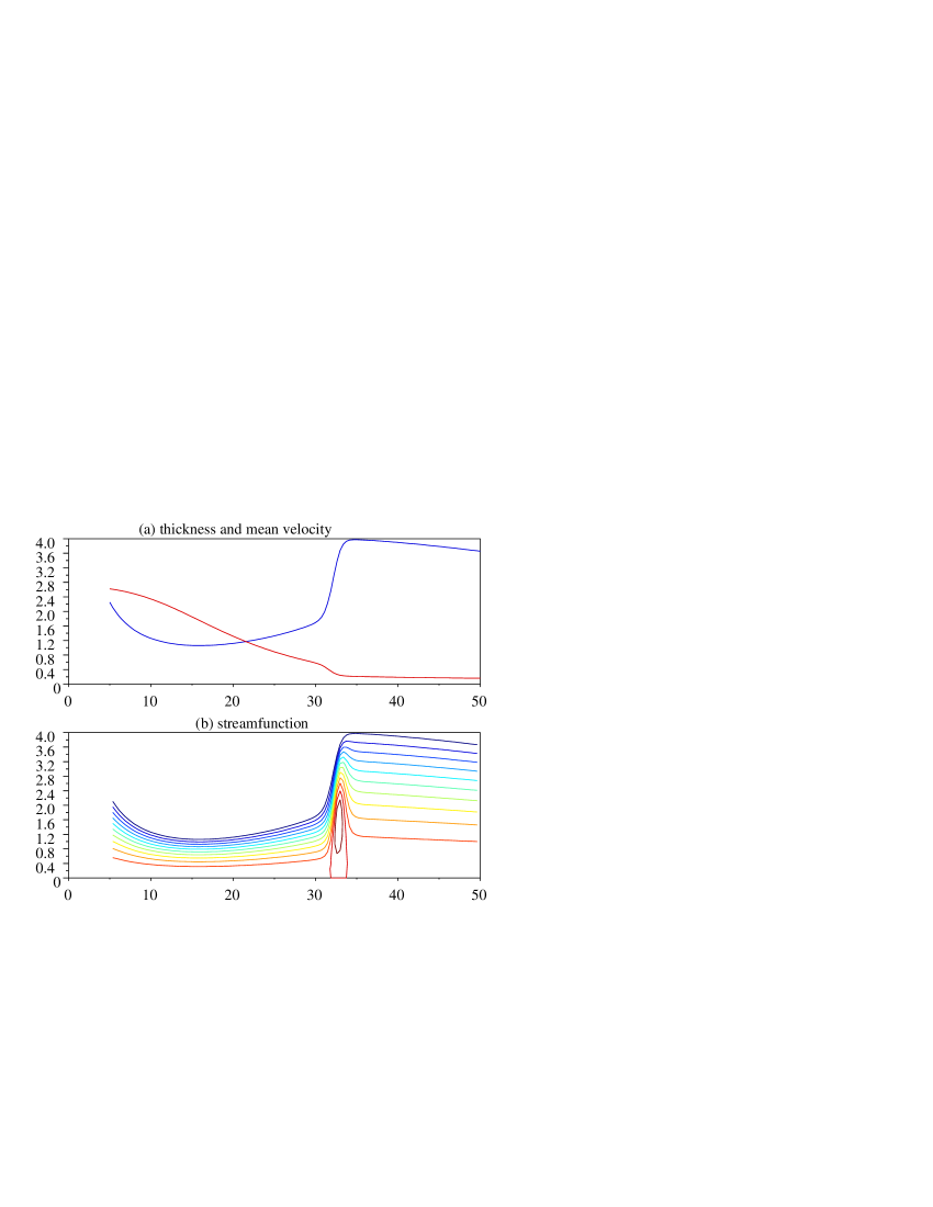
The above equations may be integrated in time to see evolving dynamics in a radial flow. Here we focus only upon steady solutions obtained by fixing an inlet condition of flow leaving the faucet with prescribed thickness and velocity; in Figure 7 the flow has and at radius , and exiting the domain with some prescribed mean velocity at large distance, at in Figure 7. Newton iteration then finds the solutions for fluid thickness and mean velocity shown in Figure 7(a). See the flow spreads out in a thin () fast flow before undergoing a hydraulic jump at distance to a thick () slow flow. The streamlines in in Figure 7(b), obtained from the velocity fields (46–47), show the presence of a recirculation under the jump as also seen in the experiments cited by Watanabe, Putkaradze and Bohr [41]. Our model expressed in depth averaged quantities resolves such nontrivial internal flow structures.
The steady flow in Figure 7 is near the limit of applicability of the model. Although the free surface looks steep in the figure, the slope is everywhere less than which, although less than the limit (57) identified earlier, is about as large as one could reasonably use. For interest, other lateral derivatives have the following ranges: , and . We also find the hydraulic jump with recirculation in less extreme flows than the one shown in Figure 7. However, we have not yet found any flows with an extra eddy at the surface of the hydraulic jump as reported for experiments with larger jumps [41, §2.1].
6.2 Flow outside a cylinder resolves evolving beads
Thin film flow on the outside or the inside of circular cylinders or tubes are important in a number of biological and engineering applications. For example, Jensen [15] studied the effects of surface tension on a thin liquid layer lining the interior of a cylindrical and curving tube and derived a corresponding evolution equation in the lubrication approximation. Our model (52–53) could be used to extend his modelling to flows with inertia. Similarly, Atherton & Homsy [2], Kalliadasis & Chang [16] and Kliakhandler et al. [18] considered coating flow down vertical fibres and similarly derived nonlinear lubrication models. Here we record the model (52–53) as it appears in full for flows both inside and outside a circular cylinder. The specific model for a circular tube which is bent and twisted is left for later work.
Use a coordinate system with the axial coordinate and the angular coordinate; denote the averaged axial and angular velocities by with components by and , respectively. The substrate has scale factors and where is the radius of the cylinder, and curvatures and where the upper/lower sign is for flow outside/inside of the cylinder. Then the model on a cylinder is, where here ,
| (62) | |||||
| (63) | |||||
| (64) | |||||
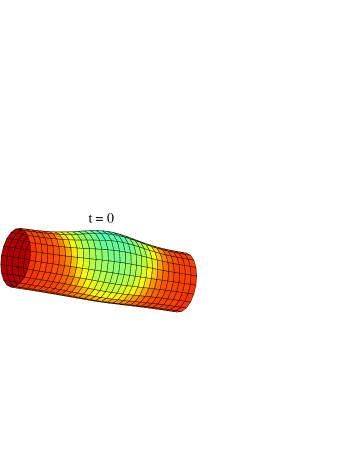
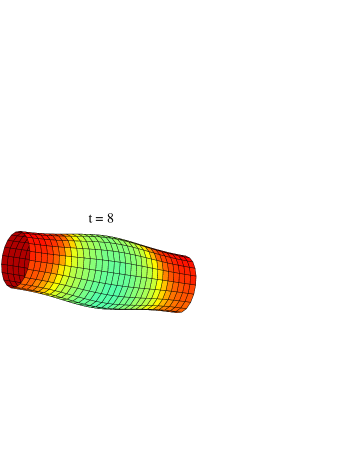
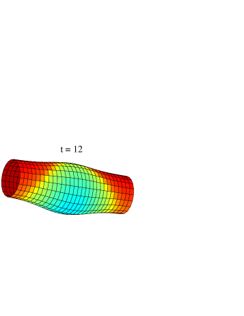
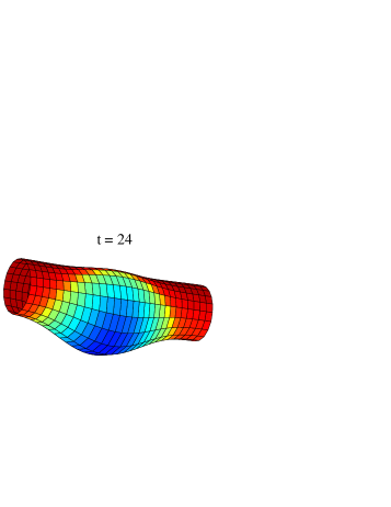
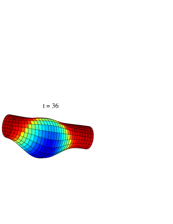
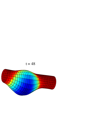
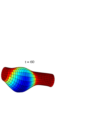
For a nontrivial example, see the beading of fluid on a thin fibre in Figures 1 and 2: gravity first rather quickly moves a lump of fluid to below the horizontal cylinder of the fibre; thereafter, surface tension more slowly gathers more fluid into the beading fluid which beads both below and above the fibre; gravity causes the fluid bead to stabilise off the centre of the fibre (curiously, there is more in the bead above the fibre than in the original lump); and finally the bead slides along the fibre as it is angled downwards a little. The three time scales in this evolution, the fast gravity forced flow, the slower surface tension driven flow, and the even longer term sliding, are captured in this model.
Simply obtain axisymmetric flows by setting to zero any derivatives with respect to , and also setting as non-zero values would break the symmetry. The equation for then just describes the decay of angular flow around the cylinder so also set . Thus the axisymmetric model is
| (65) | |||||
| (66) | |||||
recall that the upper/lower sign is for flow outside/inside of the cylinder. As in lubrication models [36, p254], see that surface tension on the cylinder acts through the term in (66) or (63) rather like a radially outwards body force such as the term in (63).
6.3 Flow about a small channel grows vortices
Consider the flow on a substrate with a small channel aligned downhill. We compare this viscous flow with the high Reynolds number experiments of Bousmar [5, 4] who modelled turbulent flow over flood plains and channels in a flume with water of variable depth but of the order of 5 cm deep.
First create the coordinate system. Bousmar’s channel and flood plain had constant shape along the stream, the depth only varied across the stream. Thus here let be the along stream coordinate, be the horizontal distance across the stream on the substrate,444There is no good reason for using the variable name for distance horizontally across the stream, only that it is next to the letter in the alphabet. In this subsection the variable is not used to indicate any sort of radius. and measure distance normal to the substrate. The curved substrate is located a distance from the -plane in a normal direction, see the example in the middle curve of Figure 8(a). Using, for this subsection, , and as the vertical and two horizontal unit vectors, the unit vectors, scale factors and curvature of the substrate coordinate system are555Useful relationships are: , , and .
This expression for the curvature is well known. Note: the normal coordinate is not the vertical coordinate, and so a flat fluid surface located at, say, the location of the reference -plane is represented by the varying . Similarly nontrivial, as the channel slopes down at an angle radians to the horizontal and not sideways tilted, the gravitational forcing is in the direction
| (67) |
This coordinate system suits any flow where the substrate is almost arbitrarily curved in only one direction, not just flow along a channel.666The model (68–70) reduces to that for the flow outside/inside a cylinder, (62–64), when and the substrate scale factors are set to and (only the direction of gravity (67) is incorrect). This algebraic connection occurs despite the cylinder not being strictly encompassed by a depth below any reference plane. Indeed the beading flow on a cylinder shown in Figures 1 and 2 was actually obtained using code for the model (68–70) of this subsection.
Second, computer algebra gives the model on this substrate as, where here ,
| (68) | |||||
| (69) | |||||
| (70) | |||||
| (a) | 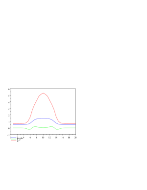 |
|---|---|
| (b) | 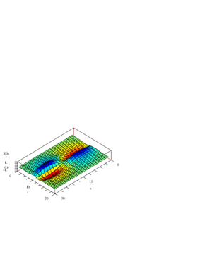 |
Lastly, as expected, simulations show that fast flow develops in the deeper channel and slow flow on the shallow regions, see Figure 8(a). However, the shear in the mean downstream velocity, Figure 8(a), is unstable to relatively weak horizontal vortices that grow in the shear and travel downstream, see them in the mean lateral velocity shown in Figure 8(b);777The vortices apparent in Figure 8(b) fill the computational domain and thus may be an artifice of the domain size. However, otherwise identical simulations on twice the channel length show twice as many vortices, whereas simulations in a domain half as long again show a rich modulation among vortices of roughly the shown length. We deduce that the displayed vortices are not solely an artifice of the computational domain. analogous notable vortices were observed by Bousmar [5, 4] in their turbulent flows. As also noted by Bousmar, see that the vortices here similarly extend into the shallows, albeit weakly.
The simulation reported here has a change in depth of the substrate sufficiently big so that the nonlinear nature of the derived model is certainly essential: Decré & Baret [10, p155] comment that nonlinear theories are needed in viscous flow if the change in substrate profile is bigger than half the shallow fluid depth; here the factor is about three, that is, six times the linear limit identified by Decré & Baret.
6.4 Flow on the outside of a sphere
For flow on the outside of a sphere we use a coordinate system with the co-latitude coordinate, the azimuthal (longitude) coordinate, and co-latitude and azimuthal velocity components and respectively. The substrate has scale factors and where is the radius of the sphere, and curvatures . Note: on a sphere every point is an umbilical point; nonetheless, the earlier analysis is valid in this conventional spherical coordinate system. Then the model on a sphere is, where here ,
| (71) | |||||
| (72) | |||||
| (73) | |||||
These models look horribly complicated but recall that depending upon the application, simpler truncations are often appropriate; two such examples are (5) and (54). These models have the assurance of centre manifold theory that all physical effects are included to the controlable specified accuracy.
7 Conclusion
We systematically analysed the Navier-Stokes equations for the flow of a thin layer of a Newtonian fluid over an arbitrarily curved substrate. The resulting general model (52–53) resolves the dynamical effects and interactions of inertia, surface tension, and a gravitational body force as well as the substrate curvature. We presented evidence towards the end of §5 that this model applies to flows where the lateral gradients of the fluid thickness are somewhat less than , see the more precise limit (57), and (in §4) where the time scales of the flow are reasonably longer than the decay of the second lateral shear mode, that is, longer than . The centre manifold paradigm for dynamical modelling is based upon actual solutions of the governing Navier-Stokes equations, parametrised in terms of cross-layer averages. Further the paradigm implicitly arranges the interaction terms between various physical processes to support flexible truncation of the model as appropriate for different parameter regimes; thus the relatively complex model (52–53) may be justifiably simplified as needed by your application.
To illustrate a range of applications we briefly reported some simulations of: wave transitions on a sloping substrate, Faraday waves on a vibrating flat plate, and a viscous hydraulic jump in radial flow, see §6.1; the formation and sliding of beads on a cylindrical fibre with surface tension and gravity, see §6.2; and the generation of vortices in the shear flow between a channel and surrounding shallows, see §6.3. These simulations demonstrate the resolution of the complex interactions between the varied physical processes encompassed by the model.
Acknowledgment:
we thank the Australian Research Council for a grant to help support this work.
Appendix A Computer algebra derives the model
The reduce888At the time of writing, information about
reduce was available from Anthony C. Hearn, RAND, Santa
Monica, CA 90407-2138, USA. mailto:reduce@rand.org
program which performs the derivation of centre manifold model is
listed below. A little explanation is usefully given first. Observe
that program variables are typeset in teletype font.
-
•
The physical coordinate system within the program is with scale factors , velocity field and pressure . Scale factors of the substrate are and , whereas those evaluated on the free surface are and .
-
•
Expressions are written in terms of a stretched coordinate system , , , so that the free surface of the fluid film is simply . In the program we use . Then spatio-temporal derivatives transform by the chain rule
as coded.
-
•
The amplitudes of the model are with
h(m,n)denoting the spatial derivative and similarly foruu(m,n)andww(m,n). The evolution of these quantities is given by
The correctness of the results of this program depend only upon the correct coding of the physical equations. The algebraic machinations are repeated until the residual of the fluid differential equations and boundary conditions are zero to the requisite order.
Comment Constructs slowly-varying lubrication model of thin
film 3D fluid flows on arbitrarily curved 2D substrates.
Allows for large changes in film thickness.  Incorporates
surface tension, gravity, inertia, slip.  The coordinate
system is (x,z,y), velocity (u,w,v), scale factors
(h1,h2,1).
Last updated 16 Sept 2003;
% improve printing appearance
on div; off allfac; on revpri;
factor d,h,uu,ww,re,gravity,betag,gr,we,k1,k2,sk;
% use operator h(m,n) to denote df(h,x,m,z,n)
operator h;
depend h,xs,zs,ts;
let { df(h(~m,~n),xs) => h(m+1,n)
     ,df(h(~m,~n),zs) => h(m,n+1)
     ,df(h(~m,~n),xs,zs) => h(m+1,n+1)
     ,df(h(~m,~n),ts) => df(gh,xs,m,zs,n) };
% principal curvatures of the substrate
operator k1;
depend k1,xs,zs;
let { df(k1(~m,~n),xs) => k1(m+1,n)
     ,df(k1(~m,~n),zs) => k1(m,n+1) };
operator k2;
depend k2,xs,zs;
let { df(k2(~m,~n),xs) => k2(m+1,n)
     ,df(k2(~m,~n),zs) => k2(m,n+1) };
operator uu; operator ww;
depend uu,xs,zs,ts;
depend ww,xs,zs,ts;
let { df(uu(~m,~n),xs) => uu(m+1,n)
     ,df(ww(~m,~n),xs) => ww(m+1,n)
     ,df(uu(~m,~n),zs) => uu(m,n+1)
     ,df(ww(~m,~n),zs) => ww(m,n+1)
     ,df(uu(~m,~n),ts) => df(gu,xs,m,zs,n)
     ,df(ww(~m,~n),ts) => df(gw,xs,m,zs,n) };
% use stretched coords: ys=y/h(x,z,t), xs=x, zs=z, ts=t
depend xs,x,y,z,t;
depend zs,x,y,z,t;
depend ys,x,y,z,t;
depend ts,x,y,z,t;
let { df(~a,x) => df(a,xs)-ys*h(1,0)/h(0,0)*df(a,ys)
    , df(~a,z) => df(a,zs)-ys*h(0,1)/h(0,0)*df(a,ys)
    , df(~a,t) => df(a,ts)-ys*gh/h(0,0)*df(a,ys)
    , df(~a,y) => df(a,ys)/h(0,0)
    };
% some abbreviations with appropriate scalings
kx:=d*k1(0,0)$ kz:=d*k2(0,0)$
eta:=h(0,0)$ etax:=d*h(1,0)$ etaz:=d*h(0,1)$
% scale factors of coord system: substrate, fluid & surface
depend m1,xs,zs;
depend m2,xs,zs;
h1:=m1*(1-kx*eta*ys)$
h2:=m2*(1-kz*eta*ys)$
hh1:=sub(ys=1,h1)$
hh2:=sub(ys=1,h2)$
% gravitational body force
depend g1,xs,zs;
depend g2,xs,zs;
depend gy,xs,zs;
let { df(g1,xs) => -rh2*df(h1,z)*g2+m1*k1(0,0)*gy
    , df(g1,zs) => rh1*df(h2,x)*g2
    , df(g2,zs) => -rh1*df(h2,x)*g1+m2*k2(0,0)*gy
    , df(g2,xs) => rh2*df(h1,z)*g1
    , df(gy,xs) => -m1*k1(0,0)*g1
    , df(gy,zs) => -m2*k2(0,0)*g2
    };
% computes mean across fluid layer
operator mean; linear mean;
let{ mean(ys^~n,ys)=> 1/(n+1)
    ,mean(ys,ys)=>1/2
    ,mean(1,ys)=>1 };
% solves -df(p,ys)=rhs s.t. sub(ys=1,p)=0
operator psolv; linear psolv;
let {psolv(ys^~n,ys) => (1-ys^(n+1))/(n+1)
    ,psolv(ys,ys) => (1-ys^2)/2
    ,psolv(1,ys) => (1-ys) };
% solves df(u,ys,2)=rhs s.t. sub(ys=0,u)=0 & mean(u)=0
% and df(v,ys,2)=rhs s.t. sub(ys=0,u)=0 & mean(v)=0
operator usolv; linear usolv;
let {usolv(ys^~n,ys) => (ys^(n+2)-2*ys/(n+3))/(n+2)/(n+1)
    ,usolv(ys,ys) => (ys^3-2*ys/4)/3/2
    ,usolv(1,ys) => (ys^2-2*ys/3)/2 };
% may derive model in special geometries if activated
if 0 then % flat substrate in Cartesian
let { k1(~p,~q)=>0, m1=>1
    , k2(~p,~q)=>0, m2=>1 }
else if 0 then % cylindrical substrate of radius rad
% x1 axial distance & x2 is angle around
% sk=+1 is flow outside cyl, sk=-1 is flow inside cyl
let { k1(~p,~q)=>0 , m1=>1
    , k2(0,0)=>-sk/rad , sk^2=>1
    , k2(~p,~q)=>0 when p+q>0 , m2=>rad }
else if 1 then begin % substrate depth(zs) below reference
% s=x1 longitudinal distance & r=x2 is cross stream location
% dd=df(depth,x2), m2=\sqrt{1+dd^2}, k2=-dd'/m2^3
depend dd,zs;
let { k1(~p,~q)=>0, m1=>1
    , k2(~p,~q)=>0 when p>0
    , df(m2,xs)=>0, df(m2,zs)=>-dd*m2^2*k2(0,0)
    , df(dd,zs)=>-m2^3*k2(0,0)
    , dd^2=>m2^2-1 } end
else if 0 then % flat substrate in polar coords
% x1 radial distance & x2 is angle around
let { k1(~p,~q)=>0 , m1=>1
    , k2(~p,~q)=>0 , m2=>xs }
else if 0 then % outside spherical coords x1=colat x2=long
let { k1(0,0)=>-1/rad
    , k1(~p,~q)=>0 when p+q>0 , m1=>rad
    , k2(0,0)=>-1/rad
    , k2(~p,~q)=>0 when p+q>0 , m2=>rad*sin(xs) } ;
% centre subspace and null evolution
u:=d*2*ys*uu(0,0); w:=d*2*ys*ww(0,0); v:=0; p:=0;
gh:=0; gu:=0; gw:=0;
% and linear approx to various reciprocals
% rh1, rh2 are the approx of 1/h1, 1/h2
rh1:=1/m1$ rh2:=1/m2$ rhh1:=rh1$ rhh2:=rh2$
% Use d to count number of uu, ww and derivatives of x & z
% Throw away this order or higher in uu, ww, d/dx & d/dz
let {d^4=>0, gam^8=>0};
gravity:=d^2*gr; % gravity is the coefficient/order of gravity terms
% Iterate until converges
it:=0$
repeat begin
   write it:=it+1;
   % approximate mean curvature of the surface
   curv:=sub(ys=1,kx+kz +d*rh1*rh2*(df(h2*rh1*etax,x)
             +df(h1*rh2*etaz,z)) +(kx^2+kz^2)*eta);
   % free-surface deviatoric stress (Batchelor, p600)
   txx:=sub(ys=1,2*d*(rhh1*df(u,x)+rhh1*rhh2*df(h1,z)*w
                 +rhh1*v*df(h1,y)));
   txz:=sub(ys=1,d*(rhh2*df(u,z)+rhh1*df(w,x)
                 -rhh1*rhh2*(df(h1,z)*u+df(h2,x)*w)));
   txy:=sub(ys=1,hh1*df(rh1*u,y)+rhh1*d*df(v,x));
   tzz:=sub(ys=1,2*d*(rhh2*df(w,z)+rhh1*rhh2*df(h2,x)*u
                 +rhh2*v*df(h2,y)));
   tzy:=sub(ys=1,hh2*df(rh2*w,y)+rhh2*d*df(v,z));
   tyy:=sub(ys=1,2*df(v,y));
   % omega=curl(q) => del^2q=-curl(omega) (Batchelor p599)
   o1:=rh2*(d*df(v,z)-df(h2*w,y));
   o2:=rh1*(df(h1*u,y)-d*df(v,x));
   oy:=rh1*rh2*(d*df(h2*w,x)-d*df(h1*u,z));
   % vertical momentum & normal surface stress
   begin scalar veq,ns;
   veq:=re*( df(v,t)+d*u*rh1*df(v,x)+v*df(v,y)
            +d*w*rh2*df(v,z)+d*m1*k1(0,0)*rh1*u^2
        +d*m2*k2(0,0)*rh2*w^2 )
        +df(p,y)-gravity*gy+rh1*rh2*d*(df(h2*o2,x)-df(h1*o1,z));
   ns:=(hh2^2*etax^2*txx+2*hh1*hh2*etax*etaz*txz
       -2*hh1*hh2^2*etax*txy -2*hh1^2*hh2*etaz*tzy
       +hh1^2*etaz^2*tzz+hh1^2*hh2^2*tyy)
       -sub(ys=1,p)*((hh2*etax)^2+(hh1*etaz)^2+(hh1*hh2)^2)
       -we*curv*((hh2*etax)^2+(hh1*etaz)^2+(hh1*hh2)^2);
   ok:=if (veq=0)and(ns=0) then 1 else 0;
   pd:=eta*psolv(veq,ys)+ns*(rhh1*rhh2)^2;
   p:=p+pd;
   end;
   % x1-momentum & tangential stress on FS
   begin scalar ueq,ts1,gud,ubed;
   ueq:=re*( df(u,t)+d*u*rh1*df(u,x)+v*df(u,y)
            +d*w*rh2*df(u,z)+d*w*rh1*rh2*(u*df(h1,z)
        -w*df(h2,x))-d*m1*k1(0,0)*rh1*v*u )
        +rh1*d*df(p,x)-gravity*g1+rh2*(d*df(oy,z)-df(h2*o2,y));
   ts1:=((hh1^2*hh2-hh2*etax^2)*txy
         +hh1*hh2*etax*(tyy-txx)-hh1^2*etaz*txz
         -hh1*etax*etaz*tzy )*rhh1^2*rhh2
         -(1-gam)*sub(ys=1,u)/eta;
   ubed:=sub(ys=0,-u);
   ok:=if ok and(ueq=0)and(ts1=0)and(ubed=0) then 1 else 0;
   gud:=(-mean(ueq*ys,ys)-ts1/eta)*3/2;
   gu:=gu+gud/re/d;
   u:=u+usolv(ueq+2*ys*gud,ys)*eta^2+ubed;
   end;
   % x2-momentum & tangential stress on FS
   begin scalar weq,ts2,gwd,wbed;
   weq:=re*( df(w,t)+d*u*rh1*df(w,x)+v*df(w,y)
            +d*w*rh2*df(w,z)+d*u*rh1*rh2*(w*df(h2,x)
        -u*df(h1,z))-d*m2*k2(0,0)*rh2*v*w )
        +rh2*d*df(p,z)-gravity*g2+rh1*(df(h1*o1,y)-d*df(oy,x));
   ts2:=((hh1*hh2^2-hh1*etaz^2)*tzy
       +hh1*hh2*etaz*(tyy-tzz)-hh2*etax*etaz*txy
       -hh2^2*etax*txz)*rhh1*rhh2^2
       -(1-gam)*sub(ys=1,w)/eta;
   wbed:=sub(ys=0,-w);
   ok:=if ok and(weq=0)and(ts2=0)and(wbed=0) then 1 else 0;
   gwd:=(-mean(weq*ys,ys)-ts2/eta)*3/2;
   gw:=gw+gwd/re/d;
   w:=w+usolv(weq+2*ys*gwd,ys)*eta^2+wbed;
   end;
   % continuity & bed
   begin scalar ceq;
   ceq:=-( d*df(h2*u,x)+d*df(h1*w,z)+df(h1*h2*v,y))/m1/m2;
   ok:=if ok and(ceq=0) then 1 else 0;
   v:=v+eta*int(ceq,ys);
   end;
   % uu and ww represent weighted mean velocity
   begin scalar ueq,weq;
   ueq:=uu(0,0)*d-mean(u*h2,ys)/m2;
   weq:=ww(0,0)*d-mean(w*h1,ys)/m1;
   ok:=if ok and(weq=0)and(ueq=0) then 1 else 0;
   u:=u+2*ys*ueq;
   w:=w+2*ys*weq;
   end;
   % refine approx of h1 and h2
   h1eq:=rh1*h1-1$ rh1:=rh1-h1eq/m1; rhh1:=sub(ys=1,rh1);
   h2eq:=rh2*h2-1$ rh2:=rh2-h2eq/m2; rhh2:=sub(ys=1,rh2);
   write ok:=if ok and(h1eq=0)and(h2eq=0) then 1 else 0;
   % kinematic BC on FS
   gh:=sub(ys=1,v-u*rh1*etax-w*rh2*etaz);
   showtime;
end until ok or(it>19);
if 0 then begin % get shear stress on the substrate
    txy:=sub(ys=0,hh1*df(rh1*u,y)+rhh1*d*df(v,x))$
    tzy:=sub(ys=0,hh2*df(rh2*w,y)+rhh2*d*df(v,z))$
    gam:=1;
    on rounded;
    print_precision 4;
    coeffn(txy,d,1);
    coeffn(tzy,d,1);
    coeffn(txy,d,2);
    coeffn(tzy,d,2);
    coeff(gu,d);
    coeff(gw,d);
end;
end;
References
- [1] R. W. Atherton and G. M. Homsy. Use of symbolic computation to generate evolution equations and asymptotic solutions to elliptic equations. J. Comp. Phys., 13:45–58, 1973.
- [2] R. W. Atherton and G. M. Homsy. On the derivation of evolution equations for interfacial waves. Chem. Eng. Comm., 2:57–77, 1976.
- [3] G. K. Batchelor. An introduction to fluid dynamics. Cambridge University Press, 1979.
- [4] D. Bousmar and Y. Zech. Large-scale coherent structures in compound channels. Technical report, Universitié Catholique de Louvain, 2003.
- [5] Didier Bousmar. Flow modelling in compund channels: momentum transfer between main channel and prismatic and non-prismatic floodplains. PhD thesis, Universitié Catholique de Louvain, 2002.
- [6] J. Carr. Applications of centre manifold theory, volume 35 of Applied Math. Sci. Springer-Verlag, 1981.
- [7] H. C. Chang. Wave evolution on a falling film. Annu. Rev. Fluid Mech., 26:103–136, 1994.
- [8] Hsueh-Chia Chang, Evgenya Demekhin, and Sergey S. Saprikin. Noise-driven wave transitions on a vertically falling film. J. Fluid Mech., 462:255– 283, 2002.
- [9] S. M. Cox and A. J. Roberts. Initial conditions for models of dynamical systems. Physica D, 85:126–141, 1995.
- [10] Michel M. J. Decré and Jean-Christophe Baret. Gravity-driven flows of viscous liquids over two-dimensional topographies. J. Fluid Mech., 487:147 –166, 2003.
- [11] Th. Gallay. A center-stable manifold theorem for differential equations in banach spaces. Commun. Math. Phys, 152:249–268, 1993.
- [12] J. B. Grotberg. Pulmonary flow and transport phenomena. Annu. Rev. Fluid Mech., 26:529–571, 1994.
- [13] H. W. Guggenheimer. Differential geometry. McGraw-Hill Book Company, Inc, 1963.
- [14] M. Hărăguş. Model equations for water waves in the presence of surface tension. Eur. J. Mech, 15:471–492, 1996.
- [15] O. E. Jensen. The thin liquid lining of a weakly curved cylindrical tube. J. Fluid Mech, 331:373–403, 1997.
- [16] S. Kalliadasis and H.-C. Chang. Drop formation during coating of vertical fibres. J. Fluid Mech., 261:135–168, 1994.
- [17] H. S. Kheshgi. Profile equations for film flows at moderate Reynolds numbers. AIChE Journal, 35:1719–1727, 1989.
- [18] I. L. Kliakhandler, S. H. Davis, and S. G. Bankoff. Viscous beads on vertical fibre. J. Fluid Mech., 429:381–390, 2001.
- [19] U. Lange, K. Nandakumar, and H. Raszillier. Symbolic computation as a tool for high-order long-wave stability analysis of thin film flows with coupled transport processes. J. Comput. Phys., 150:1–16, 1999.
- [20] G. N. Mercer and A. J. Roberts. A centre manifold description of contaminant dispersion in channels with varying flow properties. SIAM J. Appl. Math., 50:1547–1565, 1990.
- [21] G. N. Mercer and A. J. Roberts. A complete model of shear dispersion in pipes. Jap. J. Indust. Appl. Math., 11:499–521, 1994.
- [22] J. Miles and D. Henderson. Parametrically forced surface waves. Annu. Rev. Fluid Mech., 20:143–165, 1990.
- [23] J. A. Moriarty, L. W. Schwartz, and E. O. Tuck. Unsteady spreading of thin liquid films with small surface tension. Phys. Fluids A, 3(5):733–742, 1991.
- [24] A. Oron, S. H. Davis, and S. G. Bankoff. Long-scale evolution of thin liquid films. Rev. Mod. Phys., 69:931–980, 1997.
- [25] Marc Perlin and William W. Schultz. Capillary effects on surface waves. Annu. Rev. Fluid Mech., 32:241–274, 2000.
- [26] T. Prokopiou, M. J. Mccready, and H. C. Chang. Wave transitions on horizontal gas sheared liquid films. Technical report, Preprint, 1991.
- [27] Th. Prokopiou, M. Cheng, and H. C. Chang. Long waves on inclined films at high Reynolds number. J. Fluid Mech., 222:665–691, 1991.
- [28] N. M. Ribe. Bending and stretching of thin viscous sheets. J. Fluid Mech., 433:135–160, 2001.
- [29] A. J. Roberts. The application of centre manifold theory to the evolution of systems which vary slowly in space. J. Austral. Math. Soc. B, 29:480–500, 1988.
- [30] A. J. Roberts. The utility of an invariant manifold description of the evolution of a dynamical system. SIAM J. Math. Anal., 20:1447–1458, 1989.
- [31] A. J. Roberts. A sub-centre manifold description of the evolution and interaction of nonlinear dispersive waves. In L. Debnath, editor, Nonlinear waves, chapter 9, pages 127–156. World Sci, 1992.
- [32] A. J. Roberts. Low-dimensional models of thin film fluid dynamics. Phys. Letts. A, 212:63–72, 1996.
- [33] A. J. Roberts. Low-dimensional modelling of dynamics via computer algebra. Computer Phys. Comm., 100:215–230, 1997.
- [34] A. J. Roberts. An accurate model of thin 2d fluid flows with inertia on curved surfaces. In P. A. Tyvand, editor, Free-surface flows with viscosity, volume 16 of Advances in Fluid Mechanics Series, chapter 3, pages 69–88. Comput Mech Pub, 1998.
- [35] G. J. Roskes. Three-dimensional long waves on a liquid film. Phys. Fluids, 13:1440–1445, 1969.
- [36] R. Valery Roy, A. J. Roberts, and M. E. Simpson. A lubrication model of coating flows over a curved substrate in space. J. Fluid Mech., 454:235–261, 2002.
- [37] K. J. Ruschak. Coating flows. Annu. Rev. Fluid Mech., 17:65–89, 1985.
- [38] L. W. Schwartz and D. E. Weidner. Modeling of coating flows on curved surfaces. J. Engrg Maths, 29:91–103, 1995.
- [39] L. W. Schwartz, D. E. Weidner, and R. R. Eley. An analysis of the effect of surfactant on the levelling behaviour of a thin coating layer. Langmuir, 11:3690–3693, 1995.
- [40] S. A. Suslov and A. J. Roberts. Proper initial conditions for the lubrication model of thin film fluid flow. Technical report, [http://arXiv.org/abs/chao-dyn/9804018], 1998.
- [41] Shinya Watanabe, Vachtang Putkaradze, and Tomas Bohr. Integral methods for shallow free-surface flows with separation. J. Fluid Mech., 480:233–265, 2003.
- [42] S. D. Watt and A. J. Roberts. The accurate dynamic modelling of contaminant dispersion in channels. SIAM J. Appl Math, 55(4):1016–1038, 1995.