Efficient algorithm for detecting unstable periodic orbits in chaotic systems

Abstract

We present an efficient method for fast, complete, and accurate detection of unstable periodic orbits in chaotic systems. Our method consists of a new iterative scheme and an effective technique for selecting initial points. The iterative scheme is based on the semi-implicit Euler method, which has both fast and global convergence, and only a small number of initial points is sufficient to detect all unstable periodic orbits of a given period. The power of our method is illustrated by numerical examples of both two- and four-dimensional maps.

It has now been a widely accepted notion that unstable periodic orbits (UPOs) constitute the most fundamental building blocks of a chaotic system [1]. Theoretically, the infinite number of UPOs embedded in a chaotic invariant set provides a skeleton of the set, and many dynamical invariants of physical interest, such as the natural measure, the spectra of Lyapunov exponents and fractal dimensions, as well as other statistical averages of physical measurements, can be computed from the infinite set of UPOs in a fundamental way [2]. In Hamiltonian systems, the quantum mechanical density of states in the semiclassical regime can be expressed explicitly in terms of UPOs of the corresponding classical dynamics [3]. The knowledge of UPOs is also of significant experimental interest because they provide a way to characterize and understand the chaotic dynamics of the underlying system [4]. All these call for efficient techniques for detecting UPOs in chaotic systems.

Systematic detection of a complete set of UPOs of high periods embedded in a chaotic set even in situations where the system’s equations are known is, however, an extremely difficult problem. A fundamental reason is that the number of UPOs grows exponentially as the period increases at a rate given by the topological entropy of the chaotic set. The basic requirements for a good detection algorithm are, therefore, fast convergence and the ability to yield complete set of UPOs [5].

Recently, a general algorithm for detecting UPOs in chaotic systems was proposed by Schmelcher and Diakonos (SD) [6] who, for the first time, computed UPOs of high periods for systems such as the Ikeda-Hammel-Jones-Moloney map [7]. The success of the SD method relies on a globally convergent iterative scheme: convergence to UPOs can be achieved, in principle, from any initial point. However, as we will discuss shortly, this method is not very efficient from the standpoint of convergence, neither does it provide a satisfactory test for the completeness of the detected UPOs. As a matter of fact, for the Ikeda-Hammel-Jones-Moloney map, only UPOs of periods up to 13 were reported in Ref. [6], and one of the UPOs of period 10 was not detected.

The aim of this Letter is to present an efficient method for detecting UPOs in general chaotic systems. Our new iterative scheme is based on the semi-implicit Euler method [8] and has the following favorable properties: near an orbit point it exhibits a fast convergence similar to that of the traditional Newton-Raphson (NR) method, while away from the orbit points it is similar to the SD method and, therefore, is globally convergent. Another key ingredient of our method is that we select initial points based on the observation that using orbit points of UPOs of other periods to initialize the search for UPOs of a given period is much more effective than using randomly selected points in the phase space or in the attractor. We find, in most cases, it is sufficient to use only orbit points of period $p-1$ in order to detect all UPOs of period $p$. With such a strategy, we are able to compute UPOs for, say, the Ikeda-Hammel-Jones-Moloney map, of periods up to 22 for a total of over $10^{6}$ orbit points using roughly the same amount of computation required by the SD method to compute all UPOs of periods up to 13 that have less than 6000 orbit points [9]. Due to its efficiency, our method allows us to compute UPOs in higher-dimensional systems, which we illustrate using a four-dimensional chaotic map.

We begin by describing the NR and the SD methods. Consider an $N$-dimensional chaotic map: ${\bf x}_{n+1}={\bf f}({\bf x}_{n})$. The orbit points of period $p$ can be detected as zeros of the following function:

$${\bf g}({\bf x})={\bf f}^{(p)}({\bf x})-{\bf x}\>,$$ (1)

where ${\bf f}^{(p)}({\bf x})$ is the $p$-times iterated map of ${\bf f}({\bf x})$. The process of finding zeros of ${\bf g}({\bf x})$ usually begins with the choice of initial point ${\bf x}_{0}$ followed by the computation of successive corrections: ${\bf x}_{\mathrm{n}ew}={\bf x}_{\mathrm{o}ld}+\delta{\bf x}$, which converge to the desired solution. In the NR method, the corrections are calculated from a set of $N$ linear equations:

$$-{\bf J}({\bf x})\delta{\bf x}={\bf g}({\bf x})\>,$$ (2)

where ${\bf J}({\bf x})=\partial{\bf g}/\partial{\bf x}$ is the Jacobian matrix. The NR method has excellent convergence properties, approximately doubling the number of significant digits upon every iteration, provided that the initial point is within the linear neighborhood of the solution. While it is relatively easy to find suitable initial points for very small periods (using, for example, uniform grid, iterations of the map, or random number generator), the method becomes impractical for UPOs of high periods because the volume of the basin from which ${\bf x}_{0}$ can be chosen decreases exponentially as the period increases. On the other hand, in the SD method, the corrections are determined as follows:

$$\delta{\bf x}=\lambda{\bf C}{\bf g}({\bf x})\>,$$ (3)

where $\lambda$ is a small positive number and ${\bf C}$ is an $N\times N$ matrix with elements $C_{ij}\in\{0,\pm 1\}$ such that each row or column contains only one element that is different from zero. With an appropriate choice of ${\bf C}$ and a sufficiently small value of $\lambda$ the above procedure can find any periodic point of a chaotic system. The main advantage of the SD method is that the basin of attraction of each UPO extends far beyond its linear neighborhood, so most initial points converge to a UPO. In fact, the basins of attraction of individual orbit points completely fill a region in the phase space, and any initial point in this region converges to an orbit point.

Schmelcher and Diakonos tested their method by computing the UPOs for the Hénon map and other simple maps, for which the UPOs are known from methods specific to these maps [5]. They also applied the method to the Ikeda-Hammel-Jones-Moloney map, for which no special technique for computing UPOs was previously available. The method appears to be particularly useful when detecting for each period the least unstable periodic orbits [10]. However, if the goal is to determine complete sets of UPOs of increasingly higher periods, the SD method becomes inefficient due to the following two reasons: (i) the convergence rate of Eq. (3) is much slower than that of the NR method, so it takes significantly more steps to reach the desired accuracy [11]; and (ii) even though the SD scheme is globally convergent, the basins of attraction of individual UPOs are interwoven in a complicated manner, so it is extremely difficult to determine which initial point converges to a particular UPO. Because of this difficulty, the SD method cannot guarantee the detection of all UPOs of a given period.

To overcome the problem of slow convergence, while retaining the global convergence property, we propose the following iteration scheme:

$$[{\bf 1}\beta g({\bf x})-{\bf C}{\bf J}({\bf x})]\delta{\bf x}={\bf C}{\bf g}({\bf x})\>,$$ (4)

where $g({\bf x})\equiv||{\bf g}({\bf x})||\geq 0$ is the length of the vector, $\beta>0$ is an adjustable parameter, and ${\bf C}$ is the same

FIG. 1.: Shown with thick lines are the basins of convergence of (a) the Newton-Raphson (NR) method, (b) the Schmelcher-Diakonos (SD) method with $0<\lambda<0.3568$ and ${\bf C}=1$, and (c) our method with $\beta=4.0$ and ${\bf C}=1$ to the zeros of a function $\cos(x^{2})$ in the interval $(-3,3)$. Arrows indicate the direction of convergence and large dots are the zeros to which the methods converge.

matrix as in Eq (3). In the vicinity of an UPO, the function $g({\bf x})$ tends to zero and the NR method is restored. In fact, it is straightforward to verify that the above scheme retains the quadratic convergence. On the other hand, away from the solution and for sufficiently large values of $\beta$, our scheme is similar to Eq. (3) and thus almost completely preserves the global convergence property of the SD method. This similarity is easily understood, since Eq. (3) is the Euler method with step size $\lambda$ for solving the following system of ODEs:

$$\frac{{\mathrm{d}}{\bf x}}{{\mathrm{d}}s}={\bf C}{\bf g}({\bf x}).$$ (5)

On the other hand, Eq. (4) is the semi-implicit Euler method [8] with step size $h=1/\beta g({\bf x})$ for solving the same system of ODEs. Consequently, with sufficiently small step size, both methods closely follow the solutions to Eq. (5) and thus share the global convergence property.

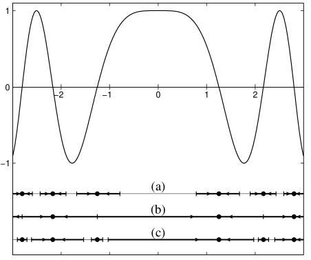
To illustrate and contrast the convergence properties of the NR, the SD, and our methods, we consider the following simple example: finding zeros of the function $g(x)=\cos(x^{2})$ in the interval $(-3,3)$. The basins of convergence for each method are shown in Fig. 1 with the thick arrows. The NR method converges to all six zeros and the basins are essentially within the linear neighborhood of each point [12]. The SD method converges to the solution $g(x_{0})=0$ if $0<\lambda<2/g^{\prime}(x_{0})$ and ${\bf C}=-{\mathrm{s}ign}(g^{\prime}(x_{0}))$. Diagram (b) in Fig. 1 shows the basin of convergence for $0<\lambda<0.3568$ and ${\bf C}=1$. Obvious is the global character of convergence to zeros with negative function derivatives, while zeros with positive derivatives serve as basin boundaries. With ${\bf C}=-1$ the convergence directions are reversed. The result of applying our iteration scheme with $\beta=4.0$ and ${\bf C}=1$ to the same function is shown in the diagram (c). We see that, as in the NR method, all zeros have basins of convergence. However, the basins of zeros with negative function derivatives cover most of the interval, while the basins of other zeros, as well as the intervals between basins, are reduced and become smaller with increasing value of $\beta$. Therefore, our scheme combines the efficiency of the NR method with the global character of the SD algorithm.

FIG. 2.: Number of detected orbits for different periods in the Ikeda-Hammel-Jones-Moloney attractor given in Eq. (6). Solid dots indicate the values of $\beta$ above which we always detect a maximum number of UPOs for each period.

Another important ingredient of our method lies in the selection of initial points: we find that the most efficient strategy for detecting UPOs of period $p$ is to use UPOs of other periods as initial points. This is understandable, since orbit points cover the attractor in a systematic manner, which reflects the foliation of the function ${\bf f}^{(p)}({\bf x})$ and its iterates. In cases of the Hénon and the Ikeda-Hammel-Jones-Moloney maps, we are able to detect all UPOs of period $p$ using only orbit points of period $p-1$, provided that period $p-1$ orbits exist. In more complicated cases of higher-dimensional maps, this simple strategy leaves a small fraction of UPOs undetected [13]. However, in all cases, we are able to find these UPOs using period $p+1$ points (first we use incomplete set of period $p$ orbits to find period $p+1$ points and then use them to complete the detection of period $p$ orbits). The main advantage of using orbit points of neighboring periods as initial points is that once we establish the strategy for smaller periods, it works in a similar manner for the detection of UPOs of large period. This allows us to claim with confidence that we detect all UPOs of increasingly longer periods for general multi-dimensional chaotic maps.

We now apply our method to detecting UPOs for the following Ikeda-Hammel-Jones-Moloney map [7]:

$$x^{\prime} = a+b(x\cos{\phi}-y\sin{\phi})\>,$$ (6)

$$y^{\prime} = b(x\sin{\phi}+y\cos{\phi})\>,$$ (7)

where $\phi=k-\eta/(1+x^{2}+y^{2})$, and the parameters are chosen such that the map has a chaotic attractor: $a=1.0$, $b=0.9$, $k=0.4$, and $\eta=6.0$. Detection of UPOs proceeds as follows: UPOs of period 1 and 2 are quickly found using several initial points on the attractor. Starting from $p=3$ we use only orbit points of period $p-1$ as initial points. We choose ${\bf C}$ from the set of five matrices $\{{\bf C}_{k}|k=1,\ldots,5\}$ provided in Ref. [6], where ${\bf C}_{1}={\bf 1}$ is the identity matrix. The iteration sequence computed from Eq. (4) is terminated when it either converges to an orbit point or leaves the chaotic attractor. The average number of iterations increases linearly with $\beta$, which is understandable since $||\delta{\bf x}||\approx 1/\beta$ for large $\beta$ and away from an orbit point. However, a small fraction of initial points produces very long sequences which neither converge to an UPO nor leave the attractor. In order to limit the amount of unproductive computation, we set the maximum number of iterations to 4-6 times $\beta$, which is sufficient for the majority of iterates to be terminated properly. The quadratic convergence of our scheme allows us to achieve, without much computational effort, accuracy limited only by the computer round-off error. Once the sequence converges to an orbit point, we check whether it belongs to a yet undetected UPO, and if so, we compute the rest of the orbit points by iterating the map and refining the solutions with a couple of NR steps [we simply set $\beta=0$ in Eq. (4) ].

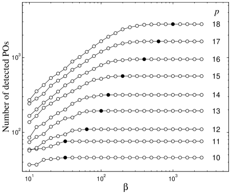
Figure 2 shows the number of detected UPOs of periods 10 through 18 using different values of $\beta$ in the range from 10 to 3000. Note that for every period there exists a value $\beta=\beta_{\mathrm{m}in}(p)$ above which we are guaranteed to find a maximum number of UPOs. This feature of our scheme strongly suggests that the detected orbits constitute a complete set of UPOs for each period. Since $\beta_{\mathrm{m}in}(p)$ is approximately proportional to ${\mathrm{e}}^{\alpha p}$, where $\alpha$ is a positive constant, we can estimate the value of $\beta$ necessary to find all UPOs of increasingly longer periods. The numbers of the UPOs for periods up to 13 agree with those of Schmelcher and Diakonos [6] except for period 10, where we have detected one additional orbit. The number of orbits of periods 14 through 22, which were not reported previously, are given in Table I.

TABLE I.: Number of distinct UPOs, $n(p)$, and the total number of orbit points or period $p$, $N(p)$, for the Ikeda attractor given by Eq. (6). Note that $N(p)$ also includes orbit points whose periods are factors of $p$.

$p$	$n(p)$	$N(p)$
14	317	4 511
15	566	8 517
16	950	15 327
17	1 646	27 983
18	2 799	50 667
19	4 884	92 797
20	8 404	168 575
21	14 700	308 777
22	25 550	562 939

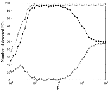
If we monitor the number of orbits detected with different matrices ${\bf C}$, we note that, for a wide range of values of $\beta$, after we use identity matrix ${\bf C}_{1}$, only a few UPOs remain undetected. For example, with $\beta=5000$ and ${\bf C}={\bf C}_{1}$ in Eq. (4), our method detects 14 699 orbits of period 21, and only one new orbit is detected with ${\bf C}={\bf C}_{2}$. To understand this feature of our method, which is common to all the maps tested, we show in Fig. 3, for the chaotic attractor in Eq. (6), the number of period 13 orbits detected with ${\bf C}_{1}$ (solid dots) and the number of additional orbits detected with ${\bf C}_{k}$, $k=2,\ldots,5$, (triangles). For $100<\beta<1000$, almost all UPOs are detected with ${\bf C}$ being the identity matrix. At larger values of $\beta$ the number of thus detected orbits decreases, but the remaining orbits are always detected with other matrices. For $\beta>10^{5}$ the numbers converge to those of the SD iteration scheme, where about half of the orbits are detected with ${\bf C}_{1}$ and the other half with ${\bf C}_{2}$ and ${\bf C}_{3}$. This behavior of our scheme follows directly from the convergence considerations of Fig. 1 and results in a greatly improved efficiency compared to either the NR or the SD methods.

Finally, we briefly describe the performance of our method for other maps. In case of the Hénon map our algorithm works extremely well and, for the standard parameter values of $(a,b)=(1.4,0.3)$, detects all UPOs up to period 29 with $\beta<500$, ${\bf C}={\bf C}_{1}$ and ${\bf C}_{2}$, and using for initialization only orbit points of period $p-1$. We have also applied our algorithm to detecting UPOs in the following four-dimensional map: Two coupled Ikeda maps with coupling in the form: $\phi_{(1,2)}=k-\eta/(1+x_{(1,2)}^{2}+y_{(1,2)}^{2})+2\pi\varepsilon(x_{(2,1)}-x_{(1,2)})$, and the parameters are chosen such that the system has two positive Lyapunov exponents. We estimate the topological entropy in this system to be $h_{\mathrm{T}}\approx 1.6$, and thus the number of orbits grows extremely fast with increasing orbit length. We have detected complete sets of UPOs up to period 7 with $\beta<1000$. We have found that the reliability of the algorithm was not affected by the increased dimensionality of the system. Even though the number of possible matrices ${\bf C}$ in four dimensions is 384, only a dozen of them are needed to detect all UPOs. The necessary set of matrices ${\bf C}$ can be selected empirically when detecting short UPOs and then used in the detection of longer orbits.

FIG. 3.: Detection of UPOs of period 13 in the Ikeda-Hammel-Jones-Moloney attractor. The number of orbits detected with ${\bf C}_{1}$ is shown with solid dots, while triangles represent the number of additional orbits detected with ${\bf C}_{k}$, $k=2,\ldots,5$. The total number of detected orbits is shown with open circles.

In conclusion, we have proposed an efficient algorithm for the detection of UPOs in chaotic systems and have successfully detected large number of UPOs in several two- and higher-dimensional maps. Our method allows for a verification of the completeness of the detected orbits and high accuracy limited only by the round-off error.

This work was supported by AFOSR under Grant No. F49620-98-1-0400 and by NSF under Grant No. PHY-9722156.

REFERENCES

- [1] D. Auerbach, P. Cvitanović, J.-P. Eckmann, G. H. Gunaratne, and I. Procaccia, Phys. Rev. Lett. 58, 2387 (1987); G. H. Gunaratne and I. Procaccia, Phys. Rev. Lett. 59, 1377 (1987); D. Auerbach, B. O’Shaughnessy, and I. Procaccia, Phys. Rev. A 37, 2234 (1988); P. Cvitanović and B. Eckhardt, Phys. Rev. Lett. 63, 823 (1989); D. Auerbach, Phys. Rev. A 41, 6692 (1990); P. Cvitanović, Focus Issue on Periodic Orbit Theory, Chaos 2, 1992.
- [2] C. Grebogi, E. Ott, and J. A. Yorke, Phys. Rev. A 37, 1711 (1988); Y.-C. Lai, Y. Nagai, and C. Grebogi, Phys. Rev. Lett. 79, 649 (1997).
- [3] M. C. Gutzwiller, Chaos in Classical and Quantum Mechanics (Springer, New York, 1990).
- [4] D. P. Lathrop and E. J. Kostelich, Phys. Rev. A 40, 4028 (1989); D. Pierson and F. Moss, Phys. Rev. Lett. 75, 2124 (1995); D. Christini and J. J. Collins, Phys. Rev. Lett. 75, 2782 (1995); X. Pei, and F. Moss, Nature (London) 379, 619 (1996); B. Hunt and E. Ott, Phys. Rev. Lett. 76, 2254 (1996); P. So, E. Ott, S. J. Schiff, D. T. Kaplan, T. Sauer, and C. Grebogi, Phys. Rev. Lett. 76, 4705 (1996); P. So, E. Ott, T. Sauer, B. J. Gluckman, C. Grebogi, and S. J. Schiff, Phys. Rev. E 55, 5398 (1997).
- [5] Particular methods exist for specific systems or in special cases, such as the method by Biham and Wenzel [O. Biham and W. Wenzel, Phys. Rev. Lett. 63, 819 (1989)] for the Hénon map for which a Hamiltonian-like function can be found with extrema located at the orbit points of UPOs, and the method by Hansen [K. Hansen, Phys. Rev. E 52, 2388 (1995)] which is applicable to two-dimensional maps if the symbolic dynamics of the map is known and well ordered.
- [6] P. Schmelcher and F. K. Diakonos, Phys. Rev. Lett. 78, 4733 (1997); Phys. Rev. E 57, 2739 (1998).
- [7] K. Ikeda, Opt. Commun. 30, 257 (1979); S. M. Hammel, C. K. R. T. Jones, and J. Moloney, J. Opt. Soc. Am. B 2, 552 (1985).
- [8] W. H. Press, S. A. Teukolsky, W. T. Vetterling, and B. P. Flannery, Numerical Recipes in Fortran, 2nd ed. (Cambridge University Press, Cambridge, 1992).
- [9] It is practically impossible to use the SD method to detect complete sets of UPOs for periods above 20 because the amount of computation required grows exponentially at a much higher rate than that of our method.
- [10] F. K. Diakonos, P. Schmelcher, and O. Biham, Phys. Rev. Lett. 81, 4349 (1998).
- [11] Indeed, close to a zero point, the corrections from Eq. (3) are proportional to the deviation (linear convergence), while corrections determined from the NR method yield an error that is proportional to the square of the deviation (quadratic convergence).
- [12] Even though the Newton-Raphson method generally has a fractal basin structure, we show only intervals adjacent to the solution, as they are the most reliable source of starting points.
- [13] For relatively short orbits we verify the completeness of the detected sets by initializing our iteration scheme on a fine grid of initial points.