Noise-amplitude dependence of the invariant density for noisy, fully chaotic one-dimensional maps

Abstract

We present some analytic, non-perturbative results for the invariant density $\rho(x)$ for noisy one-dimensional maps at fully developed chaos. Under periodic boundary conditions, the Fourier expansion method is used to show precisely how noise makes $\rho(x)$ absolutely continuous and smoothens it out. Simple solvable models are used to illustrate the explicit dependence of $\rho(x)$ on the amplitude $\eta$ of the noise distribution, all the way from the case of zero noise ($\eta\rightarrow 0$) to the completely noise-dominated limit ($\eta=1$).

PACS Nos.   05.45.+b, 05.40.+j

1 INTRODUCTION

One-dimensional (1D) maps exhibiting chaotic behaviour have been used as effective models to describe a wide variety of physical processes ranging from irregular behaviour in electronic circuits and chemical reactions to turbulence [1,2]. In particular, probabilistic or statistical approaches (involving, for instance, invariant measures on attractors) enable us to by-pass the limitations imposed by extreme sensitivity to initial conditions, and compute various quantities of interest in terms of statistical averages [3-5]. A considerable body of mathematically rigorous results on 1D discrete-time dynamics is also available [6,7]. As random noise is inevitably present in physical systems, much effort has been put in to understand the effects of noise upon different aspects of chaotic dynamics, including invariant densities and related quantities [5, 8-17]. As much (but not all) of this work is based on numerical analysis or simulation, analytical results are of importance - especially so if they are non-perturbative in nature, i.e., if they are valid for arbitrarily large noise amplitudes.

In this paper, we re-visit 1D maps in the regime of fully-developed chaos, in the presence of uncorrelated noise [18,19]. With the addition of noise, the evolution equation becomes a stochastic difference equation, thereby making the system effectively infinite-dimensional. Imposing periodic boundary conditions, the Fourier transform method [10,11] is used to establish some non-perturbative results for the invariant density $\rho(x)$. In Sec. 2, we show how the addition of noise of arbitrarily small amplitude can make $\rho(x)$ absolutely continuous in the interval. In Sec. 3, we consider a noise density that has a single non-trivial Fourier mode, and show that $\rho(x)$ is also locked in at the same mode, but with a phase shift. In Sec. 4 we examine the dependence of $\rho(x)$ on the amplitude of the noise density, varying the latter over the full range from zero (the noise-free limit) to unity (the completely noise-dominated limit). We conclude with a few remarks on the effect of noise on the Lyapunov exponent.

2 CONTINUITY OF THE INVARIANT DENSITY

We consider 1D endomorphisms $x_{n+1}=f(x_{n})\,,\;n=0,1,\cdots\,,\;x_{n}\in[-1,1]\,\equiv\,\mbox{I}$, exhibiting fully developed chaos with invariant density $\rho^{(0)}(x)$. In the presence of additive noise,

$$x_{n+1} = f(x_{n})\,+\,\xi_{n+1}$$ (1)

where $\langle\xi_{n}\rangle\,=\,0,\;\langle\xi_{n}\,\xi_{n^{\prime}}\rangle\,=\,\langle\xi^{2}\rangle\,\delta_{nn^{\prime}}$. We use periodic boundary conditions, so that the normalized noise distribution $g(\xi)$ is also a periodic function with fundamental interval I. The invariant density $\rho(x)$ for the noisy map (1) satisfies the perturbed Frobenius - Perron equation [5]

$$\rho(x) = \int_{\mbox{I}}\;dy\,g(x-f(y))\,\rho(y)\;.$$ (2)

The Fourier expansions of $\rho$ and $g$ are

$$\rho(x)=\frac{1}{2}\,\sum_{n=-\infty}^{\infty}\,\tilde{\rho}_{n}\,\exp(i\pi nx)\;,\;g(\xi)=\frac{1}{2}\,\sum_{n=-\infty}^{\infty}\,\tilde{g}_{n}\,\exp(i\pi n\xi)\,,$$ (3)

where

$$\tilde{\rho}_{n}\,=\,\int_{\mbox{I}}\;dx\,\rho(x)\,\exp(-i\pi nx)\;,\;\tilde{g}_{n}\,=\,\int_{\mbox{I}}\;d\xi\,g(\xi)\,\exp(-i\pi n\xi)\,.$$ (4)

On substituting Eqs. (3) and Eqs. (4) and using the normalization of $\rho$ and $g$ ($\Rightarrow\;\tilde{\rho}_{0}\,=\,1,\;\tilde{g}_{0}\,=\,1$), Eq. (2) becomes equivalent to the following (infinite-dimensional) inhomogeneous matrix equation [10,11] for $\tilde{\rho}_{n}\,,\;n\neq 0\,$:

$$\tilde{\rho}_{n} = \tilde{g}_{n}\,S_{n0}\,+\,{\sum_{m}}^{\prime}\,\tilde{g}_{n}\,S_{nm}\,\tilde{\rho}_{m}$$ (5)

where ${\sum}^{\prime}$ stands for a summation over all non-zero integers. The elements of the matrix $S$ are given by

$$S_{nm} = \frac{1}{2}\,\int_{\mbox{I}}\;dy\,\exp[i\pi(my-nf(y))]\,.$$ (6)

Iteration of Eq. (5) provides a fast-converging means of numerical solution, once the $\tilde{g}_{n}$ are specified from the noise distribution concerned. The unperturbed (or noise-free) case is recovered on replacing $g(\xi)$ by $\delta(\xi)$, i.e., by setting $\tilde{g}_{n}\,=\,1$ for all $n$.

It turns out that exact solutions for the invariant density $\rho(x)$ can be obtained from Eq. (5) in several important cases by exploiting the symmetries, if any, that the matrix $S$ may happen to possess [17]. For instance, if $S_{n0}\,=\,0$ for all $n\,\neq\,0$, both $\rho^{(0)}(x)$ and $\rho(x)$ reduce to the constant density 1/2. Again, suppose the noise density $g(\xi)$ is symmetric about its mean value zero (a reasonable assumption), so that $\tilde{g}_{n}\,=\,\tilde{g}_{-n}$. Then, if $S_{nm}$ is even [respectively, odd] in the index $m$, while $S_{n0}$ is odd [respectively, even] in the index $n$, only the leading term in the iterative solution of Eq. (5) survives. This leads to the exact solution

$$\rho(x) = \frac{1}{2}\,\sum_{n=-\infty}^{\infty}\,\tilde{g}_{n}\,S_{n0}\exp(-i\pi nx)\,.$$ (7)

Puting in the definitions of $\tilde{g}_{n}$ and $S_{n0}$, Eq. (7) can be re-written in the form

$$\rho(x) = \frac{1}{2}\,\int_{\mbox{I}}\;dy\,g(x-f(y))\,.$$ (8)

We shall use these results in Sec. 4 to study analytically the dependence of the invariant density on the amplitude of the noise distribution.

Here, we wish to point out a simple way of understanding precisely how the addition of noise leads, in general, to a smoother invariant density [20,21]. Consider the noise-free case: The Fourier coefficients of $\rho^{(0)}(x)$ are given by

$$\tilde{\rho}_{n}^{(0)}=S_{n0}\,+\,{\sum_{m}}^{\prime}S_{nm}\,\tilde{\rho}_{m}^{(0)}=S_{n0}\,+\,{\sum_{m}}^{\prime}S_{nm}\,S_{m0}\,+\,{\sum_{m}}^{\prime}\,{\sum_{l}}^{\prime}S_{nm}\,S_{ml}\,S_{l0}\,+\,\cdots$$ (9)

The asymptotic (large $n$) behaviour of $\tilde{\rho}_{n}^{(0)}$ is thus controlled by $S_{nm}$. If $\tilde{\rho}_{n}^{(0)}\sim\,n^{-1}$, then $\rho^{(0)}(x)$ has finite discontinuities in I – including, possibly, the end points $\pm 1$, as we have used periodic boundary conditions. Now consider what happens when noise is added. If $g(\xi)$ is continuous, then $\tilde{g}_{n}\sim n^{-2}$. Even if $g(\xi)$ has finite jumps in I (including, possibly, at the end points $\pm 1$), its aymptotic behaviour is at least $O(n^{-1})$ [22]. It follows at once from Eq. (5) that the asymptotic behaviour of $\tilde{\rho}_{n}$ is improved to $\tilde{\rho}_{n}\,=\,O(n^{-1-\alpha})$ where $\alpha>0$. Consequently, $\sum\,\tilde{\rho}_{n}\,\exp(i\pi nx)$ converges absolutely in I, and $\rho(x)$ becomes continuous everywhere, including the end points. (That is, $\rho(-1)\,=\,\rho(1).$) Explicit illustrations will be given subsequently.

3 EXACT SOLUTION FOR ‘SINGLE - MODE’
NOISE DENSITY

We show now that an interesting form of “mode-locking” occurs if the noise density has a single wavelength, i.e., Fourier component. The corresponding noise density is given by the one-parameter family of functions

$$g(\xi) = \frac{1}{2}\,[1\,+\,(-1)^{r-1}\,\cos\pi r\xi]\,,$$ (10)

where $r$ is an integer. Correspondingly,

$$\tilde{g}_{n} = \delta_{n,0}\,+\,\frac{1}{2}\,(-1)^{r-1}(\delta_{n,r}\,+\,\delta_{n,-r})\,.$$ (11)

Hence the only nonvanishing Fourier coefficients $\tilde{\rho}_{n}\;(n\neq 0)$ are $\tilde{\rho}_{r}$ and $\tilde{\rho}_{-r}\,=\,{\tilde{\rho}_{r}}^{*}$. Using the relation $S_{-n,-m}\,=\,S_{n,m}^{*}$, we find from Eq. (5) the solution

$$\tilde{\rho}_{r} = \frac{2(-1)^{r-1}\,S_{r0}\,-\,S_{r0}\,S_{rr}^{*}\,+\,S_{r0}^{*}\,S_{-rr}^{*}}{4-4(-1)^{r-1}\mbox{Re}\,S_{rr}\,+\,|S_{rr}|^{2}\,-\,|S_{-rr}|^{2}}\,.$$ (12)

Writing $\tilde{\rho}_{r}\,=\,|\tilde{\rho}_{r}|\,\exp(i\phi)$, this leads to the result

$$\rho(x) = \frac{1}{2}\,+\,|\tilde{\rho}_{r}|\,\cos(\pi rx+\phi)\,.$$ (13)

The invariant density is therefore ‘locked in’ at the same wavelength as the noise density, with a phase shift. The amplitude and phase shift $\phi$ depend on the map $f$ through the matrix elements of $S$ that appear in Eq. (12). It is evident that the situation corresponds to completely noise-dominated dynamics. This is brought out explicitly in the example considered in the next section.

4 DEPENDENCE OF $\rho(x)$ ON THE NOISE AMPLITUDE

We want to study the explicit dependence of the invariant density on the amplitude of the noise density in a non-perturbative manner. For this purpose, we consider illustrative cases in which an exact solution for $\rho(x)$ is possible owing to symmetries present in $S_{nm}$, as indicated in Sec. 2. The noise density is taken to have a compact support $[-\eta,\eta]$ (i.e., an amplitude $\eta$). A convenient form for the normalized density $g(\xi)$ that enables us to scan the entire range of $\eta$ from 0 to 1 is

$$g(\xi)\,=\,\left\{\begin{array}[]{cc}(2\eta)^{-1}\,(1\,+\,\cos\frac{\pi\xi}{\eta})\,,&|\xi|\,<\,\eta\\ 0,&\eta\,<|\xi|\,\leq 1\end{array}\right.$$ (14)

where $0\,<\,\eta\,<\,1$. Figure 1 depicts $g(\xi)$ for $\eta\,=\,0.2$. In the limit $\eta\rightarrow\,0$, we have $g(\xi)\rightarrow\,\delta(\xi)$, or noise-free dynamics. When $\eta\rightarrow\,1$, we have the fully noise dominated case considered in the preceding section. The Fourier coefficients of $g(\xi)$ are given by

$$\tilde{g}_{n} = \frac{\sin\,(n\pi\eta)}{n\pi\eta}\,\left[1\,-\,\frac{n^{2}\,\eta^{2}}{n^{2}\,\eta^{2}\,-\,1}\right]\,.$$ (15)

To bring out all the effects of noise on $\rho(x)$ which we want to demonstrate, let us first consider the square-root cusp map (see Fig. 2)

$$x_{n+1}=f(x_{n})=1\,-\,2\,|x_{n}|^{1/2}\;\;,\;\;x_{n}\in\mbox{I}\;.$$ (16)

It is well known that this map provides a prototypical model of intermittent chaos, arising from the marginal stability of the fixed point at the left boundary, $x\,=\,-1$. However, unlike many other models of intermittency that share the latter feature, the map (16) has the non-singular invariant density [23]

$$\rho^{(0)}(x) = \frac{1\,-\,x}{2}\;\;.$$ (17)

As $f(x)$ is symmetric, we have $S_{nm}\,=\,S_{n,-m}$. Further,

$$S_{n0}\,=\,\frac{1}{2}\,\int_{\mbox{I}}\,dy\,\exp(2\pi in\sqrt{y})\,=\,\frac{(-1)^{n}}{(i\pi n)}\,=\,-S_{-n,0}\,.$$ (18)

Hence, as pointed out in Sec. 2, the exact solution for $\rho(x)$ is given by Eq. (7). We get

$$\rho(x) = \frac{1}{2}\,+\,\sum_{n=1}^{\infty}\frac{(-1)^{n}}{n\pi}\,\tilde{g}_{n}\,\sin(n\pi x)\,.$$ (19)

Putting in the expression for $\tilde{g}_{n}$ from Eq. (15) and carrying out the summations involved, we finally obtain the closed-form expression

$$\rho(x)\,=\,\left\{\begin{array}[]{lc}\frac{1}{2}\,+\,\frac{1}{2\eta}\,(1-\eta)\,(1+x)\,+\,\frac{1}{2\pi}\,\sin\,\frac{\pi(1+x)}{\eta}\,,&-1\leq x\leq-1+\eta\\ \frac{1-x}{2}\,,&-1+\eta\leq x\leq 1-\eta\\ \frac{1}{2}\,-\,\frac{1}{2\eta}\,(1-\eta)\,(1-x)\,+\,\frac{1}{2\pi}\,\sin\,\frac{\pi(x-1)}{\eta}\,,&1-\eta\leq x\leq 1\,.\end{array}\right.$$ (20)

Figure 3 shows $\rho(x)$ in the cases $\eta\,=\,0.1,\,0.2$ and 0.7 respectively. (Throughout this paper, relatively large values of $\eta$ have been chosen for clarity of illustration, and also to emphasize the non-perturbative nature of the results.) The following points are noteworthy:
(i) Both $\rho^{(0)}(x)$ and $\rho(x)$ are antisymmetric about the mean value 1/2. However, $\rho^{(0)}(-1)$ = 1 while $\rho^{(0)}(1)=0$. But $\rho(x)$ is continuous everywhere, including the end points $\pm 1\;(\rho(\pm 1)$ = 1/2), in accordance with the general result established in Sec. 2. This feature persists for arbitrarily small values of $\eta$. It is known that it is rather difficult in numerical simulations to obtain the exact result $\rho^{(0)}(x)=(1-x)/2$: a ‘boundary layer’ persists, especially near $x=-1$, in which the invariant density builds up to a value close to unity, instead of straightaway starting at that value for $x=-1$ and then decreasing linearly as $x$ increases. Our result on the continuity of $\rho(x)$ accounts for this phenomenon: noise, albeit in the form of round-off errors, is inevitably present in simulations. (ii) In the opposite, noise-dominated limit $\eta\rightarrow 1$, we find

$$\rho(x) = \frac{1}{2}\,-\,\frac{\sin\,(\pi x)}{2\pi}\;,$$ (21)

again in accord with the results of Sec. 3, in the special case $r=1,\,|\tilde{\rho}_{r}|\,=\,1/(2\pi)\,,\,\phi\,=\,\pi/2$.

Next, let us consider a simple case in which $\rho^{(0)}(x)$ has a finite jump in the interior of the interval, in order to see how the noise smoothens it out. A convenient illustration is provided by the piecewise linear map (see Fig. 4)

$$x_{n+1}\,=\,f(x_{n})\,=\,\left\{\begin{array}[]{lc}1\,-\,5|x|\,,&|x|\,\leq\frac{1}{5}\\ \frac{(1\,-\,5|x|)}{4}\,,&\frac{1}{5}\,\leq\,|x|\,\leq 1\,\,.\end{array}\right.$$ (22)

The unperturbed invariant density is the piecewise constant function

$$\rho^{(0)}(x)\,=\,\left\{\begin{array}[]{cc}\frac{4}{5}\,,&-1\leq\,x\,<0\\ \frac{1}{5}\,,&0<x\,\leq 1\end{array}\right.$$ (23)

with a jump at $x=0$. In this case, too, $S_{nm}\,=\,S_{n,-m}$, and

$$S_{n0}\,=\,-S_{-n0}\,=\,\frac{3i}{5n\pi}[1\,-\,(-1)^{n}]\,\,.$$ (24)

When noise (distributed as in Eq. (14) is added, $\rho(x)$ is found to be the following piecewise analytic function, for $\eta\,<1/2$:

$$\rho(x)\,=\,\left\{\begin{array}[]{lc}\frac{1}{2}\,+\,\frac{3}{10\eta}(1+x)\,+\,\frac{3}{10\pi}\,\sin\,\frac{\pi(1+x)}{\eta}\,,&-1\leq x\leq-1+\eta\\ \frac{4}{5}\,,&-1+\eta\leq x\leq-\eta\\ \frac{1}{2}\,-\,\frac{3x}{10\eta}\,-\,\frac{3}{10\pi}\,\sin\,\frac{\pi x}{\eta}\,,&|x|\leq\eta\\ \frac{1}{5}\,,&\eta\leq x\leq 1-\eta\\ \frac{1}{2}\,-\,\frac{3}{10\eta}(1-x)\,-\,\frac{3}{10\pi}\,\sin\,\frac{\pi(1-x)}{\eta}\,,&1-\eta\leq x\leq 1\,.\\ \end{array}\right.$$ (25)

$\rho(x)$ remains piecewise analytic for $\eta>1/2$, as well. As before, we illustrate in Fig. 5 the trends in the variation of $\rho(x)$ using large values of $\eta$ : 0.2, 0.5 and 0.7 respectively. As expected, the discontinuities that $\rho^{(0)}(x)$ has at $x=0$ and $\pm 1$ disappear in $\rho(x)$, for arbitrarily small $\eta$. As $\eta\rightarrow 1$, $\rho(x)$ tends to $1/2\,-\,(3/5\pi)\sin(\pi x)$, corroborating our result obtained for ‘single - mode’ noise.

5 CONCLUDING REMARKS

We have shown that additive noise significantly alters the invariant density for fully chaotic 1D maps: arbitrarily small amounts of noise smoothen out the density and remove any discontinuities it may have in the absence of noise, under periodic boundary conditions. One may ask whether the Lyapunov exponent $\lambda^{(0)}$ is also altered by the addition of noise [24]. While this is so in general, there is no change in $\lambda^{(0)}$ in the examples considered in Sec. 4, for the following reason: if the map $f(x)$ is an even function of $x$, so is $\ln\,|f^{\prime}(x)|$. If, further, both $\rho^{(0)}(x)\,-\,1/2$ and $\rho(x)\,-\,1/2$ are antisymmetric in $x$, it follows that the corresponding Lyapunov exponents are equal to each other, and are given by

$$\lambda^{(0)}\,=\,\lambda\,=\,\int_{0}^{1}\,dx\,\ln|f^{\prime}(x)|\,.$$ (26)

The general conclusion is as follows: if $f(x)$ is an even function in I and so is the noise density, then $\lambda$ remains equal to $\lambda^{(0)}$ provided $S_{n0}$ is odd in the index $n$, i.e., $\int_{\mbox{I}}\,dx\,\cos\,(n\pi f(x))$ vanishes for every integer value of $n$.

Figure Captions

1. Plot of $g(\xi)$ vs $\xi$ for $\eta\,=\,0.2$

2. The square-root cusp map

3. Plot of $\rho(x)$ vs $x$ for the noisy square-root cusp map corresponding to $\eta\,=\,0.1,\,0.2$ and 0.7 respectively

4. The piecewise linear map

5. Plot of $\rho(x)$ vs $x$ for the piecewise linear map corresponding to $\eta\,=\,0.2,\,0.5$ and 0.7 respectively

Figure 1:

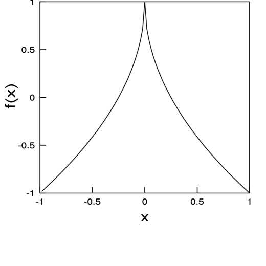
Figure 2:

Figure 3:

Figure 4:

Figure 5:

References

- [1] F. C. Moon, Chaotic Vibrations (Wiley, New York, 1987).
- [2] J. M. T. Thomson and H. B. Stewart, Nonlinear Dynamics and Chaos (Wiley, New York, 1987).
- [3] E. Ott, Chaos in Dynamical Systems (Cambridge University Press, Cambridge, 1993).
- [4] A. J. Lichtenberg and M. A. Lieberman, Regular and Chaotic Motion (Springer-Verlag, New York, 1992).
- [5] A. Lasota and M. C. Mackey, Chaos, Fractals and Noise (Springer-Verlag, New York, 1994).
- [6] W. de Melo and S. van Strien, One-Dimensional Dynamics (Springer-Verlag, New York, 1993).
- [7] A. Katok and B. Hasselblatt, Introduction to the Modern Theory of Dynamical Systems (Cambridge University Press, Cambridge, 1995).
- [8] J. P. Crutchfield, J. D. Farmer and B. A. Huberman, Phys. Rep. 92, 45 (1982).
- [9] R. Kapral, M. Schell and S. Fraser, J. Phys. Chem. 86, 2205 (1982).
- [10] S. P. Hirshman and J. C. Whitson, Phys. Fluids 25, 967 (1982).
- [11] A. B. Rechester and R. B. White, Phys. Rev. A 27, 1203 (1983).
- [12] R. Graham, Phys. Rev. A 28, 1679 (1983).
- [13] A. Lasota and M. C. Mackey, Physica D 28, 143 (1987).
- [14] E. Knobloch and J. B. Weiss, in Noise in Nonlinear Dynamical Systems, edited by F. Moss and P. V. E. McClintock (Cambridge University Press, Cambridge, 1989), Vol. 2, p. 65.
- [15] P. Talkner and P. Hänggi, in Noise in Nonlinear Dynamical Systems, edited by F. Moss and P. V. E. McClintock (Cambridge University Press, Cambridge, 1989), Vol. 2, p. 87.
- [16] G. Nicolis and V. Balakrishnan, Phys. Rev. A. 46, 3569 (1992).
- [17] V. Balakrishnan, G. Nicolis and C. Nicolis, Pramana-J. Phys. 48, 109 (1997).
- [18] If the low-dimensional dynamics arises (as it often does) as a reduced or effective description of some ‘true’ higher dimensional dynamics, the inclusion of white noise in the latter will then formally lead to colored noise in the reduced system (see , e.g., Ref. [19]). Hence it is the effects of colored rather than uncorrelated noise that we should consider. However, in practice this is ultimately a question of relative time scales in the specific problem concerned: If there is a clear separation between the characteristic time scales of the noise and the deterministic dynamics, neglecting the correlation time of the former may be quite justified.
- [19] E. Knobloch and J. E. Weiss, J. Stat. Phys. 58, 863 (1990).
- [20] For rigorous, formal results in this regard, see L. -S. Young and M. Benedicks, Ergodic Th. & Dynam. Sys. 12, 13 (1992).
- [21] This is actually quite a general phenomenon, not restricted to 1D maps. See, for example, R. F. Fox, Phys. Rev. A 42, 1946 (1990); R. F. Fox and J. Keizer, Phys. Rev. A 43, 1709 (1991); and also Ref. [16].
- [22] T. W. Korner, Fourier Analysis (Cambridge University Press, Cambridge, 1989).
- [23] P. C. Hemmer, J. Phys. A 17, L247 (1984).
- [24] L. -S. Young and F. Ledrappier, Ergodic Th. & Dynam. Sys. 11, 469 (1991).