Quantization of Multidimensional Cat Maps

¹Centro Brasileiro de Pesquisas Físicas

Rua Xavier Sigaud 150, CEP 22290-180, RJ, Rio de Janeiro, Brazil

²Comisión Nacional de Energía Atómica (CNEA),

Ave. del Libertador 8250, 1429 Buenos Aires, Argentina.

PACS:

Keywords:Dynamical Systems, Quantum maps, Quantum Chaos, ergodicity, semiclassial limit.

Abstract

In this work we study cat maps with many degrees of freedom. Classical cat maps are classified using the Cayley parametrization of symplectic matrices and the closely associated center and chord generating functions. Particular attention is dedicated to loxodromic behavior, which is a new feature of two-dimensional maps. The maps are then quantized using a recently developed Weyl representation on the torus and the general condition on the Floquet angles is derived for a particular map to be quantizable. The semiclassical approximation is exact, regardless of the dimensionality or of the nature of the fixed points.

1 Introduction

Linearization of a dynamical system near a periodic orbit is one of the most fruitful starting points for the analysis of classical motion. In its turn, the symplectic group of linear Hamiltonian systems in plane phase space is easily quantized to form the corresponding metaplectic quantum group. Essentially, the generating function for the group of canonical transformations is simply exponentiated to obtain a representation of the quantum unitary transformation.

If the chosen orbit is a point of equilibrium, the corresponding linear system belongs to the homogeneous symplectic group, characterized by a single equilibrium, usually taken as the origin. Likewise, the Poincaré map in the neighborhood of a periodic orbit is linearized into a homogeneous symplectic map with discrete time. The essential character of the motion is classified according to the eigenvalues of the symplectic matrix ${\cal M}$, that determines the evolution of phase space points $x:$

$$x^{\prime}={\cal M}x.$$ (1.1)

There may be

(a)

pairs of eigenvalues ($\lambda,\lambda^{-1});$

(b)

pairs of eigenvalues on the unit circle ($e^{i\theta},e^{-i\theta})$

(c)

quartets of general complex eigenvalues $\lambda^{\pm 1}e^{\pm i\theta}.$

On varying parameters, it is possible to obtain unit eigenvalues , or eigenvalue collisions, but the above classification is generic for a given symplectic system [1].

It is always possible to decompose such a generic linearized system into sub-systems in invariant subspaces of two dimensions, corresponding to cases (a) and (b) above, or four dimensions in case (c). Case (b) is the elliptic map, which is trivially integrable, whereas case (a) defines hyperbolic motion. This is also very simple in the linear limit, but can become a source of chaotic mixing as nonlinear perturbations are added. Alternatively, this effect is achieved by wrapping the plane space itself into a torus.

The resulting symplectomorphism of the torus is known colloquially as a cat map, characterized by a symplectic matrix with integer elements. A hyperbolic cat map is structurally stable, i.e. the orbit structure is invariant with respect to small nonlinear perturbations as a consequence of Anosov’s theorem [1]. The same is true of a four dimensional loxodromic cat map with general complex eigenvalues in case (c). These structurally invariant systems are known as Anosov systems, they are ergodic and mixing.

It follows that four dimensions is the lower bound in which we can study loxodromic periodic orbits [1], characterized by stable and unstable manifolds where the orbits spiral inwards and outwards respectively, and their effect on the quantum energy spectrum. This is the reason for their absence in all previous studies of the quantization of cat maps, though Greenman [2] has recently analyzed the periodic structure of higher dimensional classical cat maps. Dimension four is also the least dimension for the analysis of the decomposition of the neighborhood of orbits into elliptic and (real) hyperbolic components.

In some cases this decomposition is only local, because the canonical transformation that achieves it is not itself a cat map. Then the quantum quasienergy spectrum will not be decomposed into the corresponding lower dimensional spectra. In any case, all cat maps derived from each other as a result of similarity transformations involving other cat maps are equivalent: they have the same (classical and quantum) eigenvalues and the same number of fixed points. ( Note that, on the torus, a homogeneous linear map may have multiple fixed points.)

For this reason, we discuss in the next section the integer subgroup of symplectic transformations, nicknamed the feline group. For higher dimensions than two, we encounter the problem of a priori identification of a cat map. An alternative approach involves generating functions, of which there are several choices. However there is a great advantage to using generating functions that are invariant with respect to feline transformations.

In section 3 we analyze the dynamics of classical cat maps and classify four-dimensional cat maps, providing examples of various types. These examples are then quantized in section 4. They share a simplifying property that permits us to discuss the periodicity of the propagator and the exactness of the Gutzwiller trace formula, without analyzing the subtleties of general cat map quantization. This is the subject of section 5, where we determine the set of Floquet angles that allow the quantization of a given map; and study the feline invariance of the quantization.

2 Feline-invariant generating functions

A point in the even-dimensional phase space with $L$ degrees of freedom on a $2L$-torus has coordinates separated into $L$ momenta and $L$ positions, so that $x=\left(\begin{array}[]{c}p\\ q\end{array}\right)=\left(\begin{array}[]{c}p_{1},\cdots,p_{L}\\ q_{1},\cdots,q_{L}\end{array}\right)$. All the $2L$ coordinates are periodic with periods $\Delta q_{i}$ and $\Delta p_{i}$. For simplicity we will treat the case where we can choose units so that $\Delta q_{i}$ and $\Delta p_{i}$ are all equal to 1. The range of values of $x$ is then the unit $2L$-hypercube denoted from now on by $\Box.$

Let us consider then a linear automorphism on the $2L$-torus generated by the $2L\times 2L$ matrix ${\cal M}$, that takes a point $x_{-}=\left(\begin{array}[]{c}p_{-}\\ q_{-}\end{array}\right)$ to a point $x_{+}=\left(\begin{array}[]{c}p_{+}\\ q_{+}\end{array}\right):$

$$x_{+}={\cal M}x_{-}\quad\mbox{mod(1)}.$$ (2.1)

In other words, there exists an integer $2L$-dimensional vector ${\bf m}=\left(\begin{array}[]{l}m_{p}\\ m_{q}\end{array}\right),$ such that

$$x_{+}={\cal M}x_{-}-{\bf m.}$$ (2.2)

The components of ${\bf m}$ denote the winding numbers made by the point $x_{-}$ around the respective irreducible circuit on the $2L$-torus after the application of the map ${\cal M}.$ The torus will be divided into regions labeled by their respective vector ${\bf m}$. For the map to be conservative, the ${\cal M}$ matrix must be symplectic, that is

$${\cal M}^{t}{\mathfrak{J}}{\cal M}={\mathfrak{J},}$$ (2.3)

where ${\cal M}^{t}$ is the transpose of ${\cal M}$ and

$${\mathfrak{J}}=\left[\begin{array}[]{c|c}0&-1\\ \hline\cr 1&0\end{array}\right].$$ (2.4)

The matrix ${\cal M}$ must have integer coefficients for the $2L$-torus to be mapped onto itself.

For one degree of freedom ( $L=1$ ) these systems are known as Arnold’s cat maps [1]. If $|tr({\cal M})|>2$ the map has two distinct real eigenvectors, so it is ergodic, mixing and purely hyperbolic. For the case $|tr({\cal M})|<2$ there are no real eigenvectors, the map is then elliptic. For $|tr({\cal M})|=2$ there is only one real eigenvector and so the map is parabolic. For more degrees of freedom richer structure may appear, as will be discussed.

The set of matrices ${\cal M}$ satisfying (2.3) form the symplectic group, so that the matrix ${\cal M}^{\prime},$ obtained from ${\cal M}$ by the similarity transformation

$${\cal N}^{-1}{\cal M}{\cal N}={\cal M}^{\prime}$$ (2.5)

is also symplectic if the matrix ${\cal N}$ is itself symplectic and shares the same eigenvalues as ${\cal M}$. Indeed, we may consider the symplectic transformation corresponding to ${\cal M}^{\prime}$ as the same as ${\cal M}$, but viewed in an alternative symplectic coordinate system.

Consider now a product of cat maps; this must be symplectic and all the matrix elements will be integers. Since the inverse of a cat map is also a symplectic integer transformation and the unit matrix likewise, the set of cat maps is a subgroup of the symplectic group, appropriately nicknamed the feline group. Again, we may consider similarity transformations of the form (2.5) among cat maps ${\cal M}$ and ${\cal N}$ as defining essentially maps viewed by alternative symplectic coordinates on the torus.

The importance of defining equivalence classes of similar cat maps increases with the dimension of the torus. It is easy to define integer matrices and the a posteriori condition (2.3) merely restricts the value of the determinant to unity when $L=1.$ However, for $L=2$, the symplectic property already implies ten independent conditions to be satisfied by the sixteen integer matrix elements. An alternative procedure, that we adopt here, is to define the transformation implicitly by means of a generating function, thus guaranteeing (2.3). The disadvantage is now that we need to ensure that the resulting matrix ${\cal M}$ has integer entries, leading to additional restrictions on the allowed generating functions (see below ) . Nevertheless, this approach has proved very fruitful, because the quantization relies heavily on the generating function, and not on the transformation matrix itself.

The generating function in position representation for the one degree of freedom case is [3]

$$S(q_{-},q_{+},{\bf m})=\frac{1}{2{\cal M}_{21}}\left[{\cal M}_{22}q_{-}^{2}-2q_{-}(q_{+}+m_{q})+{\cal M}_{11}(q_{+}+m_{q})^{2}-2{\cal M}_{21}m_{p}q_{+}\right].$$ (2.6)

This function generates the dynamics through

$$p_{+} = \frac{\partial S(q_{-},q_{+},{\bf m})}{\partial q_{+}}$$ (2.7)

$$p_{-} = -\frac{\partial S(q_{-},q_{+},{\bf m})}{\partial q_{-}}.$$ (2.8)

Thus the quadratic part of the generating function is common to the entire torus, whereas the linear part depends on the winding vector ${\bf m}$ that changes discontinuously on the boundary of each subregion of the torus.

The weakness of the position generating function is that it transforms in a complicated way under feline similarity transformations. Only in the special case of a point transformation, that does not mix momenta with positions, will the generating function remain invariant. In contrast, the center and chord generating functions, are known to be symplectically invariant [4]. Adapted to the torus, we shall show that they can also be chosen to be invariant under feline transformations.

The starting point is to define the center point $x$ and the chord $\xi$ such that

$$x_{\pm}=x\pm\frac{1}{2}\xi,$$ (2.9)

so that the center

$$x\equiv\frac{x_{+}+x_{-}}{2}$$ (2.10)

and the chord

$$\xi\equiv x_{+}-x_{-}.$$ (2.11)

Given the initial point $x_{-}$,

$$x = \frac{1}{2}\left({\cal M}+1\right)x_{-}-\frac{{\bf m}}{2}$$ (2.12)

$$\xi = \left({\cal M}-1\right)x_{-}-{\bf m.}$$ (2.13)

Elimination of $x_{-}$, then establishes the direct relation between centers and chords:

$$x = \frac{1}{2}\frac{\left({\cal M}+1\right)}{({\cal M}-1)}\xi+({\cal M}-1)^{-1}{\bf m}$$ (2.14)

$$\xi = 2\frac{\left({\cal M}-1\right)}{\left({\cal M}+1\right)}x-2\left({\cal M}+1\right)^{-1}{\bf m}.$$ (2.15)

Center and chord generating functions respectively denoted by $S(x,{\bf m})$ and $S(\xi,{\bf m})$ are defined in [4] so that the transformation is obtained as

$$x = {\mathfrak{J}}\frac{\partial S(\xi,{\bf m})}{\partial\xi}$$ (2.16)

$$\xi = -{\mathfrak{J}}\frac{\partial S(x,{\bf m})}{\partial x}.$$ (2.17)

In analogy to the dynamics in the plane, we may consider that use of the center representation identifies the orbit with the reflection (or inversion) through $x$, because of (2.10). Hence we shall also refer to $x$ as the reflection point. The chord representation is locally equivalent to the uniform translation of phase space by the chord (2.11). Equating (2.14) with (2.16) and (2.15) with (2.17), we obtain the quadratic generating functions

$$S(x,{\bf m}) = xBx+x(B-{\mathfrak{J})}{\bf m}+f({\bf m})$$ (2.18)

$$S(\xi,{\bf m}) = \frac{1}{4}\xi\beta\xi+\frac{1}{2}\xi(\beta+{\mathfrak{J})}{\bf m}+g({\bf m})$$ (2.19)

where $B$ and $\beta$ are symmetric matrices; they are the Cayley parametrization of ${\cal M}:$

$${\mathfrak{J}}B = \frac{\left(1-{\cal M}\right)}{\left(1+{\cal M}\right)}$$ (2.20)

$${\mathfrak{J}}\beta = \frac{\left({\cal M}+1\right)}{\left({\cal M}-1\right)}$$ (2.21)

If ${\cal M}$ has an eigenvalue equal to $1$ then the $\beta$ matrix will be singular. This corresponds to a caustic of the center generating function. Whereas if ${\cal M}$ has an eigenvalue equal to $-1$, then $B$ will be a singular matrix which corresponds to a caustic of the chord generating function [4].Some useful relations obtained from (2.20) and (2.21) are

$$(B-{\mathfrak{J}}) = -2{\mathfrak{J}}\left(1+{\cal M}\right)^{-1},$$ (2.22)

$$(\beta+{\mathfrak{J}}) = -2{\mathfrak{J}}\left({\cal M}-1\right)^{-1},$$ (2.23)

$${\mathfrak{J}}B=-\frac{1}{{\mathfrak{J}}\beta}$$ (2.24)

and

$${\cal M}=\frac{\left(1-{\mathfrak{J}}B\right)}{\left(1+{\mathfrak{J}}B\right)}=\frac{\left({\mathfrak{J}}\beta+1\right)}{\left({\mathfrak{J}}\beta-1\right)}.$$ (2.25)

The functions $f({\bf m})$ and $g({\bf m})$ are arbitrary, since they only depend on the winding number ${\bf m}$, so they do not affect the transformation (2.14) or (2.15). However, the center generating function for cat maps can also be obtained directly from the map (2.2). This is a composition of the symplectic map on the plane ${\cal M}$ , whose center generating function is $S_{1}(x)=xBx,$ with the uniform translation $T_{-{\bf m}}$ of vector $-{\bf m}$ that pulls back the final point to the unit cell $\Box.$ The generating function of such a translation is [4] $S_{2}(x)=-{\bf m\wedge}x$ , also symplectically invariant. Then, using the composition law for center generating functions [4] we obtain the generating function (2.18) with

$$f({\bf m})=\frac{1}{4}{\bf m}B{\bf m.}$$ (2.26)

As in the plane case [4] generating functions are related among themselves by Legendre transformations. Thus, $S(x,{\bf m})$ is obtained from the more familiar position generating function $S(q_{-},q_{+},{\bf m})$ as

$$S(x,{\bf m})=S(q_{-},q_{+},{\bf m})+\frac{1}{2}(p_{-}+p_{+})(q_{+}-q_{-}),$$ (2.27)

whereas the relation between the chord and center generating function is

$$S(\xi,{\bf m})=\xi\wedge x-S(x,{\bf m}).$$ (2.28)

In each case, the variable absent on the left side is eliminated by requiring the right side to be stationary with respect to it. The skew product in (2.28) ,

$$\xi\wedge\eta\ \equiv\sum_{\ell=1}^{L}\left(\xi_{p_{\ell}}\eta_{q_{\ell}}-\xi_{q_{\ell}}\eta_{p_{\ell}}\right)=({\mathfrak{J}}\xi).\eta=-\xi{\mathfrak{J}}\eta,$$ (2.29)

is the symplectic area of the parallelogram formed by any pair of vectors $\xi$ and $\eta$. Then, using (2.28), for the center function with the term (2.26), we obtain the chord generating function (2.19) with

$$g({\bf m})=\frac{1}{4}{\bf m}\beta{\bf m.}$$ (2.30)

We shall label periodic points of period $l$ as $x_{l}.$ Thus, fixed points $x_{1}$ are such that the chord $\xi=0,$ or the center $x=x_{1}=({\cal M}-1)^{-1}{\bf m,}$ which inserted in (2.28) leads to

$$S(\xi=0,{\bf m})=-S(x_{1},{\bf m}).$$ (2.31)

There follows the restriction that the terms in $S(\xi,{\bf m})$ and $S(x,{\bf m})$ that depend only on ${\bf m}$ satisfy

$$f({\bf m})+g({\bf m})=\frac{1}{4}{\bf m}(\beta+B){\bf m.}$$ (2.32)

The choice (2.26) and (2.30) obviously satisfy this criterion, but another possibility is

$$f({\bf m})=\frac{1}{4}{\bf m}(B+\widetilde{{\mathfrak{J}}}){\bf m\quad}\mbox{and}\quad g({\bf m})=\frac{1}{4}{\bf m}(\beta-\widetilde{{\mathfrak{J}}}){\bf m,}$$ (2.33)

where we define the symmetric matrix

$$\widetilde{{\mathfrak{J}}}=\left[\begin{array}[]{c|c}0&1\\ \hline\cr 1&0\end{array}\right].$$ (2.34)

Using (2.33), we match the value of the action for a fixed point previously proposed by Keating [3], for the position representation

$$S(q_{-}=q_{f},q_{+}=q_{f},{\bf m})=S(x_{1},{\bf m}).$$ (2.35)

In conclusion, the center and chord generating functions for multidimensional cat maps are

$$S(x,{\bf m}) = xBx+x(B-{\mathfrak{J})}{\bf m}+\frac{1}{4}{\bf m}(B+\widetilde{{\mathfrak{J}}}){\bf m}$$ (2.36)

$$S(\xi,{\bf m}) = \frac{1}{4}\xi\beta\xi+\frac{1}{2}\xi(\beta+{\mathfrak{J})}{\bf m}+\frac{1}{4}{\bf m}(\beta-\widetilde{{\mathfrak{J}}}){\bf m.}$$ (2.37)

The corresponding generating functions for the transformation $x_{+}={\cal M}x_{-}$ in the plane are just $S(x,0)$ and $S(\xi,0)$. It is important to note that all the reflections of the torus can be obtained with center points whose coordinates are in $[0,\frac{1}{2}].$ It would thus be possible to define such center points $x^{\prime}$ as

$$x^{\prime}\equiv\frac{x_{+}+x_{-}}{2}\qquad\mbox{mod}(\frac{1}{2}).$$ (2.38)

This choice would not lead to the explicit relation (2.12) with the winding number of the transformation, but instead

$$x^{\prime}=\frac{1}{2}\left({\cal M}+1\right)x_{-}-\frac{{\bf m}^{\prime}}{2},$$ (2.39)

where ${\bf m}^{\prime}$ has coordinates ${\bf m}_{i}^{\prime}=({\bf m}_{i}$ or ${\bf m}_{i}{\bf+1}),$ so that all the coordinates of $x^{\prime}$ would be in $[0,\frac{1}{2}].$ Hence, we allow instead the center points $x,$ defined as in (2.10), to have coordinates in the full interval $[0,1],$ keeping the explicit relation with the winding number of the transformation.

As a consequence, the chords defined as in (2.11), have coordinates lying in the extended range $[-1,1].$ Thus, center points differing by integer loops around the torus are equivalent and so are chords differing by two integer loops.

$$x \equiv x+{\bf k}$$ (2.40)

$$\xi \equiv \xi+2{\bf k.}$$ (2.41)

We find that (2.40) and (2.41) imply that, in (2.14) and (2.15) respectively, the winding number ${\bf m}\,$ is equivalent to:

$${\bf m}\equiv{\bf m}^{\prime}={\bf m}+({\cal M}-1){\bf k}$$ (2.42)

in (2.14) and

$${\bf m}\equiv{\bf m}^{\prime\prime}={\bf m}-({\cal M}+1){\bf k}.$$ (2.43)

in (2.15). This implies that replacing   ${\bf m}$ by ${\bf m}^{\prime}$ in the generating function $S(\xi,{\bf m})$ will lead to equivalent center points related by (2.40). To obtain equivalent chords related by (2.41), it is necessary to replace ${\bf m}$ by ${\bf m}^{\prime\prime}\,$in the center generating function $S(x,{\bf m})$. Performing the mentioned replacements we will obtain:

$$S(\xi,{\bf m}^{\prime}) = S(\xi,{\bf m})+\xi\wedge{\bf k-}\frac{1}{2}{\bf m}\Gamma_{1}{\bf k-}\frac{1}{4}{\bf k}\Delta_{1}{\bf k}$$ (2.44)

$$S(x,{\bf m}^{\prime\prime}) = S(x,{\bf m})-2x\wedge{\bf k-}\frac{1}{2}{\bf m}\Gamma_{2}{\bf k-}\frac{1}{4}{\bf k}\Delta_{2}{\bf k,}$$ (2.45)

where

$$\Gamma_{1} = \left[\left({\mathfrak{J}}+\widetilde{{\mathfrak{J}}}\right){\cal M}+\left(\widetilde{{\mathfrak{J}}}-{\mathfrak{J}}\right)\right]$$ (2.46)

$$\Delta_{1} = \left[\left({\cal M}^{t}\widetilde{{\mathfrak{J}}}{\cal M}+\widetilde{{\mathfrak{J}}}\right)+{\cal M}^{t}\left(\widetilde{{\mathfrak{J}}}-{\mathfrak{J}}\right)+\left({\mathfrak{J}}+\widetilde{{\mathfrak{J}}}\right){\cal M}\right]$$ (2.47)

$$\Gamma_{2} = \left[\left({\mathfrak{J}-}\widetilde{{\mathfrak{J}}}\right){\cal M}+\left({\mathfrak{J}}+\widetilde{{\mathfrak{J}}}\right)\right]$$ (2.48)

$$\Delta_{2} = \left[\left({\cal M}^{t}\widetilde{{\mathfrak{J}}}{\cal M}+\widetilde{{\mathfrak{J}}}\right)-{\cal M}^{t}\left({\mathfrak{J}}+\widetilde{{\mathfrak{J}}}\right)-\left({\mathfrak{J}}-\widetilde{{\mathfrak{J}}}\right){\cal M}\right].$$ (2.49)

In this way we can restrict ${\bf m}$ to integer component vectors that lie in one of the two fundamental parallelepipeds

$$\begin{array}[]{cc}\Diamond_{\xi}=({\cal M}-1)\Box&\qquad\mbox{for }S(\xi,{\bf m})\end{array}$$ (2.51)

$$\begin{array}[]{cc}\Diamond_{x}=({\cal M}+1)\Box&\qquad\mbox{for }S(x,{\bf m})\end{array}$$ (2.53)

where $\Box$ is the unit hypercube that denotes the $2L$-torus. Hence, the different orbits denoted by a given chord $\xi$ are given by all the integer ${\bf m}$ lying in $\Diamond_{\xi}$. The number of such orbits is independent of $\xi$, so taking $\xi=0$, we equate this to the number of fixed points $\tau_{\xi}$, i.e.

$$\tau({\cal M})=|\det({\cal M}-1)|=\frac{2^{2L}}{|\det({\mathfrak{J}}\beta-1)|}\equiv\tau_{\xi}.$$ (2.54)

The different orbits that have the point $x$ as its center are denoted by all the integers ${\bf m}$ lying now in $\Diamond_{x}.$ The number of these orbits is given by the volume of $\Diamond_{x}$ which is

$$\tau(-{\cal M})=\left|\det({\cal M}+1)\right|=\frac{2^{2L}}{|\det({\mathfrak{J}}B+1)|}\equiv\tau_{x}.$$ (2.55)

Note that the number of periodic points of period two is $\tau_{\xi}\tau_{x}.$

For the matrix ${\cal M}$ to represent a $2L$-cat map it must be symplectic, so that the map is area preserving, and ${\cal M}$ must have integer entries. Let us now translate both the conditions for the $B$ and $\beta$ matrices. The first condition implies that $B$ and $\beta$ are symmetric matrices, and any symmetric matrix is associated through (2.25) to a symplectic matrix. The second condition restricts the $B$ and $\beta$ matrices to have rational entries. Indeed, following (2.20) and(2.21) we will have

$$B = \frac{\overline{B}}{\det({\cal M}+1)}\equiv\pm\frac{\overline{B}}{\tau_{x}}$$ (2.56)

$$\beta = \frac{\overline{\beta}}{\det({\cal M}-1)}=\pm\frac{\overline{\beta}}{\tau_{\xi}}$$ (2.57)

where $\overline{B}$ and $\overline{\beta}$ are symmetric matrices with integer entries and the denominators are defined by (2.54) and (2.55). It can happen that all the coefficients of the matrix $\overline{B}$ ( or $\overline{\beta}$ ) have a common factor that is not coprime with $\tau_{x}$ (respectively $\tau_{\xi}$ ). Dividing by this common factor the fraction in (2.56) ( or in (2.57) ) is reduced to the form

$$B = \pm\frac{\overline{B}^{\prime}}{\tau_{x}^{\prime}}$$ (2.58)

$$\beta = \pm\frac{\overline{\beta}^{\prime}}{\tau_{\xi}^{\prime}}.$$ (2.59)

But not any symmetric $B$ or $\beta$ matrix with rational entries guarantees that the associated symplectic matrix will have integer elements. So we must find conditions on $B$ and $\beta$ for this to occur.

The characterization of the matrices $B$ or $\beta$ requires that the corresponding transformation on the plane maps the points of an integer lattice among themselves. We will examine the case $L=1$, as the extension for many number of degrees of freedom follows easily. There are two fundamental chords corresponding to fixed points on the torus:

$$\xi_{1}=\left(\begin{array}[]{l}1\\ 0\end{array}\right)\mbox{ \qquad and \qquad}\xi_{2}=\left(\begin{array}[]{l}0\\ 1\end{array}\right),$$ (2.60)

leading to the fixed points:

$$x_{j}=\frac{1}{2}({\mathfrak{J}}\beta+1)\xi_{j\qquad,}\mbox{ with }j=1,2.$$ (2.61)

Of course, there is also $\xi_{0}=0$, but this ”plane fixed point” makes no restriction on the torus map. For the transformation to be a cat map, all the corners of the fundamental parallelogram $\Box$ must be fixed points, so, for any integers $r$ and $s$, there are integers $m_{1}$ and $m_{2}$ such that:

$$m_{1}x_{1}+m_{2}x_{2}=\left(\begin{array}[]{l}r\\ s\end{array}\right)=\frac{1}{2}({\mathfrak{J}}\beta+1)\left(\begin{array}[]{l}{m_{1}}\\ {m_{2}}\end{array}\right).$$ (2.62)

This is true if only if $2({\mathfrak{J}}\beta+1)^{-1}$ has integer entries. This condition is general for any degrees of freedom. Similarly, we find that $2({\mathfrak{J}}\beta-1)^{-1}$ having integer entries is also a necessary and sufficient condition for the corresponding ${\cal M}^{-1}$ to define a cat map. But , if ${\cal M}$ defines a cat map, so does $-{\cal M}$ with the associated chord matrix $-B.$ Therefore, it is also a necessary and sufficient condition, for a center generating function to determine a cat map, that the associated center matrix $B$ have the property that $2({\mathfrak{J}}B\pm 1)^{-1}$ be an integer matrix. Evidently we easily find a subclass of cat maps by restricting their Cayley parametrization to $B$ (or $\beta$ ) matrices of the form (2.56) such that $det(1\pm{\mathfrak{J}}B)=\pm 1,\pm 2$, then $2(1+{\mathfrak{J}}B)^{-1}$ is an integer matrix.

Although the conditions on the symmetric matrices $B$ or $\beta\,\,$to denote a cat map are not as trivial as the ones on the symplectic matrix ${\cal M},$ it is simpler to find rational symmetric matrices that fulfill the condition on $\beta$ and $B$ than to find integer symplectic matrices. The fact that $B$ or $\beta$ are symmetric and of the form (2.56) allows us to find cat maps by sampling $\left[(L)\times(2L+1)+1\right]$ integer numbers. Otherwise, to fulfill the condition (2.3), needs a loop over $(2L)^{2}$ integer coefficients.

To conclude this section, we verify the property of feline invariance for the chord and center generating functions. First, we note that, symplectic invariance in the plane [4] implies that under a symplectic coordinate transformation $x\rightarrow x^{\prime}={\cal N}x,$ $S(x,0)=S(x^{\prime},0)$ and $S(\xi,0)=S(\xi^{\prime},0),$ with $\xi^{\prime}={\cal N}\xi.$ But it is also evident that the winding number ${\bf m}$ transforms in the same manner: ${\bf m}^{\prime}={\cal N}{\bf m.}$ As far as the $x$ dependent term in $S(x,{\bf m}),$ we thus find that the effect of the feline transformation is merely that of substituting $B\rightarrow{\cal N}^{t}B{\cal N},$ and similarly the change in $S(\xi,{\bf m})$ is obtained from $\beta\rightarrow{\cal N}^{t}\beta{\cal N}.$ The constant terms $f({\bf m})$ and $g({\bf m})$ in (2.18) and (2.19) are not invariant under a feline transformation in the form (2.33) that we have chosen to match reference [3], so that it is preferable to use (2.26) and (2.30) when dealing with equivalence classes of cat maps.

It is important to note that, unlike the symmetric matrices $B$ and $\beta$, ${\mathfrak{J}}B\rightarrow{\cal N}^{-1}{\mathfrak{J}}B{\cal N}$ and ${\mathfrak{J}}\beta\rightarrow{\cal N}^{-1}{\mathfrak{J}}\beta{\cal N}$, under a similarity transformation ${\cal M}\rightarrow{\cal N}^{-1}{\cal M}{\cal N}.$ Therefor, the eigenvalues of ${\mathfrak{J}}B$ and ${\mathfrak{J}}\beta$ are feline invariant, just as those of ${\cal M}$, and can thus be used to classify cat maps.

3 Classification of classical cat maps

The periodic orbits of cat maps have been studied in great details by Percival and Vivaldi [5] and also by Keating in [3] for one degree of freedom and their results were recently extended to an arbitrary number of degrees of freedom [2]. It is shown that a point on the unit $2L$-torus is periodic if and only if all its coordinates are rational and any grid of points with rational coordinates is invariant under the action of the map. From (2.2) we can see that the periodic points $x_{l}$ of integer period $l$ are labeled by the winding numbers ${\bf m,}$ so that

$$x_{l}=\left(\begin{array}[]{l}{p_{l}}\\ {q_{l}}\end{array}\right)=({\cal M}^{l}-1)^{-1}{\bf m=}({\mathfrak{J}}\beta^{\left(l\right)}-1)\frac{{\bf m}}{2}.$$ (3.63)

Here $\beta^{\left(l\right)}$ denotes the symmetric matrix associated to ${\cal M}^{l}$ through (2.21). To have $x_{l}$ on the unit $2L$-hypercube $\Box$, ${\bf m}$ must lie within the parallelepiped formed by the action of the matrix $({\cal M}^{l}-1)$ on $\Box.$ Hence, the number of integer points ${\bf m}$ is given by its hypervolume, so that the number of periodic points with period $l$ is

$$\tau({\cal M}^{l})=|\det({\cal M}^{l}-1)|=\frac{2^{2L}}{|\det({\mathfrak{J}}\beta^{\left(l\right)}-1)|}.$$ (3.64)

According to (3.63) the periodic points of period $l$ form a lattice in phase space with rational coordinates.

The motion of any point $x_{-}=x_{1}+\delta_{-}$ near a fixed point $x_{1}$ will be

$${\cal M}x_{-}={\cal M}(x_{1}+\delta_{-})=x_{1}+{\cal M}\delta_{-}=x_{1}+\delta_{+}=x_{+}.$$ (3.65)

To determine the character of such a motion we have to study the eigenvalues and eigenvectors of the matrix ${\cal M}$:  

$$\lambda_{\cal M}^{k}=\left|\lambda_{\cal M}^{k}\right|e^{i\theta_{k}}$$ (3.66)

The modulus $\left|\lambda_{\cal M}^{k}\right|$ indicates that the motion is stretching while the argument $e^{i\theta_{k}}$ indicates rotation around the fixed point $x_{1}.$ For a symplectic matrix ${\cal M}$, if $\lambda_{\cal M}$ is an eigenvalue of ${\cal M}$ then $\lambda_{\cal M}^{*}$, $\frac{1}{\lambda_{\cal M}}$ and $\frac{1}{\lambda_{\cal M}^{*}}$ will also be eigenvalues of ${\cal M}.$

The classification of the eigenvalues is possible in either the ${\cal M},B,$ or $\beta$ descriptions. Using (2.25) we obtain the relation with the eigenvalues of ${\mathfrak{J}}B$ and ${\mathfrak{J}}\beta$ denoted respectively as $\lambda_{{\mathfrak{J}}B}$ and $\lambda_{{\mathfrak{J}}\beta},$

$$\lambda_{\cal M}=\frac{\left(1-\lambda_{{\mathfrak{J}}B}\right)}{\left(1+\lambda_{{\mathfrak{J}}B}\right)}=\frac{\left(\lambda_{{\mathfrak{J}}\beta}+1\right)}{\left(\lambda_{{\mathfrak{J}}\beta}-1\right)}$$ (3.67)

and inversely:

$$\lambda_{{\mathfrak{J}}B} = \frac{\left(1-\lambda_{\cal M}\right)}{\left(1+\lambda_{\cal M}\right)}$$ (3.68)

$$\lambda_{{\mathfrak{J}}\beta} = \frac{\left(\lambda_{\cal M}+1\right)}{\left(\lambda_{\cal M}-1\right)}=-\frac{1}{\lambda_{{\mathfrak{J}}B}}.$$ (3.69)

In this way, if $\lambda_{{\mathfrak{J}}B}$ is an eigenvalue of ${\mathfrak{J}}B,$ then $\lambda_{{\mathfrak{J}}B}^{*}$, $-\lambda_{{\mathfrak{J}}B}$ and $-\lambda_{{\mathfrak{J}}B}^{*}$ will also be. In the same way, if $\lambda_{{\mathfrak{J}}\beta}$ is an eigenvalue of ${\mathfrak{J}}\beta,$ then $\lambda_{{\mathfrak{J}}\beta}^{*}$, $-\lambda_{{\mathfrak{J}}\beta}$ and $-\lambda_{{\mathfrak{J}}\beta}^{*}$ also are.

For cat maps with $L=2$ the matrices ${\cal M},B,$ and $\beta$ will be $4\times 4$ and we then have the following generic cases for the eigenvalues

1. Elliptic: there is a conjugate pair of $\lambda_{\cal M}$ both on the unit circle and conjugate pairs of purely imaginary $\lambda_{{\mathfrak{J}}B}$ and $\lambda_{{\mathfrak{J}}\beta}.$

2. Hyperbolic: there is a pair $(\lambda_{\cal M},\frac{1}{\lambda_{\cal M}})$ on the real axis and pairs $(\lambda_{{\mathfrak{J}}B},-\lambda_{{\mathfrak{J}}B})$ and $(\lambda_{{\mathfrak{J}}\beta},-\lambda_{{\mathfrak{J}}\beta})$ on the real axis.

3. Parabolic: there are degenerate eigenvalues $\lambda_{\cal M}=\pm 1$. Then for $\lambda_{\cal M}=1,$ $\beta$ is singular and $\lambda_{{\mathfrak{J}}B}=0$; for $\lambda_{\cal M}=-1,$ $B$ is singular and $\lambda_{{\mathfrak{J}}\beta}=0$.

4. Mixed: each pair belongs to a different one of the above categories.

5. Loxodromic: the eigenvalues of ${\cal M},B,$ or $\beta$ matrices form quartets of complex eigenvectors of the form $(\lambda_{\cal M},\frac{1}{\lambda_{\cal M}},\lambda_{\cal M}^{*},\frac{1}{\lambda_{\cal M}^{*}})\,$ for the ${\cal M}$ matrix and $(\lambda_{{\mathfrak{J}}S},-\lambda_{{\mathfrak{J}}S},\lambda_{{\mathfrak{J}}S}^{*},-\lambda_{{\mathfrak{J}}S}^{*})\,$ for $S$ being one of the symmetric matrices $B$ or $\beta.$

The first three cases arise also for one degree of freedom cat maps. The case $L=2$ is the lowest number of degrees of freedom where not only elliptic, parabolic and hyperbolic fixed points will appear, but also loxodromic ones. For more degrees of freedom no new cases will occur; there is only a greater variety of mixed cases. Nongeneric possibilities arise for any dimension for continuous families of systems [1], but we do not know if there exists any corresponding cat map.

In the general case, the motion is the composition of stretching and rotation, but if the angles of the rotation are of the form $\theta_{k}=\frac{i}{j}2\pi,$ after $j\,$ applications of the map, the matrix ${\cal M}^{j}$ has only real eigenvalues that come in pairs $\left|\lambda_{\cal M}^{k}\right|^{j}$ and $\left|\lambda_{\cal M}^{k}\right|^{-j}$. The dynamics has then an ignorable coordinate; the angles are constants of the motion for ${\cal M}^{j}.$ For one degree of freedom systems, where there are only two eigenvalues, $\lambda_{\cal M}$ and $\lambda_{\cal M}^{*},$ the condition

$$Tr\left({\cal M}\right)=\lambda_{\cal M}+\lambda_{\cal M}^{*}=\mbox{integer}$$ (3.70)

implies that in the elliptic case only angles of the form $\theta_{k}=\frac{i}{j}\pi$ with $j=2$ or $3$ are allowed. This is an example of a rational restriction on $\theta_{k}$, that is, ${\cal M}^{j}$ will be the identity map. This result is in accordance with Mañe’s theorem [6] that two-dimensional symplectomorphisms are either Anosov or they have zero entropy. Nonetheless, irrational rotation angles do exist in the loxodromic or mixed cases for $L>1$.

We now turn our attention to the classification of four-dimensional cat maps. Recalling that the characteristic polynomial for any $k\times k$ matrix $A$ is

$$P_{A}(\lambda)=\det(A-\lambda)=\sum_{n=1}^{k}\alpha_{n}\lambda^{k-n},$$ (3.71)

where the $\alpha_{n}$ coefficients are given by the recurrence relation,

$$\alpha_{0} = 1,$$ (3.72)

$$\alpha_{n} = -\frac{1}{n}\sum_{i=1}^{n}\alpha_{n-i}a_{i}\qquad\mbox{ with }a_{i}=Tr(A^{i}),$$ (3.73)

we obtain that for any symmetric matrix $B$ (i.e. $B$ and $\beta$ ),

$$P_{{\mathfrak{J}}B}(\lambda)=P_{{\mathfrak{J}}B}(-\lambda)$$ (3.74)

so that

$$P_{{\mathfrak{J}}B}(\lambda)=\lambda^{4}-\frac{1}{2}b_{2}\lambda^{2}+\det B$$ (3.75)

with $b_{2}=Tr\left[\left({\mathfrak{J}}B\right)^{2}\right],($ note that $\det{\mathfrak{J}}B=\det B)$. There is a similar expression for $P_{{\mathfrak{J}}\beta}(\lambda)$, required when the center representation is singular,

$$P_{{\mathfrak{J}}\beta}(\lambda)=\lambda^{4}-\frac{1}{2}\beta_{2}\lambda^{2}+\det\beta.$$ (3.76)

where $\beta_{2}=Tr\left[\left({\mathfrak{J}}\beta\right)^{2}\right].$ For the symplectic case, we obtain

$$P_{\cal M}(\lambda)=\lambda^{4}-Tr({\cal M})\lambda+\frac{1}{2}\left[Tr({\cal M}^{2})-Tr({\cal M})^{2}\right]\lambda^{2}-Tr({\cal M})\lambda^{3}+1$$ (3.77)

which is harder to analyze, so we will perform the classification of the different behaviors using ${\mathfrak{J}}B$ or ${\mathfrak{J}}\beta$. Solving $P_{{\mathfrak{J}}B}(\lambda)=0$ using (3.75), leads to

$$\lambda_{{\mathfrak{J}}B}=\pm\sqrt{\frac{b_{2}}{4}\pm\sqrt{\left(\frac{b_{2}}{4}\right)^{2}-\det B}},$$ (3.78)

whereas

$$\lambda_{{\mathfrak{J}}\beta}=\pm\sqrt{\frac{\beta_{2}}{4}\pm\sqrt{\left(\frac{\beta_{2}}{4}\right)^{2}-\det\beta}}.$$ (3.79)

We can now classify the different behaviors according to the feline invariants of the matrix ${\mathfrak{J}}B\,$ or ${\mathfrak{J}}\beta$, the eigenvalues of the symplectic matrix ${\cal M}$ being obtained with the help of (3.67). The loxodromic behavior corresponding to four complex eigenvalues will appear if the square root term $\left[\left(\frac{b_{2}}{4}\right)^{2}-\det B\right]$ inside the square root is negative. That is, the loxodromic behavior will appear only if

$$\det B>\left(\frac{b_{2}}{4}\right)^{2}\qquad\mbox{ or equivalently }\qquad\det\beta>\left(\frac{\beta_{2}}{4}\right)^{2}.$$ (3.80)

In fig 3.1 we find a complete classification of the different types of behavior according to the feline invariants of ${\mathfrak{J}}\beta$ and the same arises for the invariants of ${\mathfrak{J}}B.$ These invariants also allow us to obtain $\tau_{\xi},\,$the number of orbits for any chord $\xi,$

$$\tau_{\xi}=\left|\frac{2^{4}}{P_{{\mathfrak{J}}\beta}(1)}\right|=\left|\frac{2^{4}\det B}{P_{{\mathfrak{J}}B}(1)}\right|,$$ (3.81)

or $\tau_{x}$ the number of orbits centered on $x$ as

$$\tau_{x}=\left|\frac{2^{4}}{P_{{\mathfrak{J}}B}(1)}\right|=\left|\frac{2^{4}\det\beta}{P_{{\mathfrak{J}}\beta}(1)}\right|.$$ (3.82)

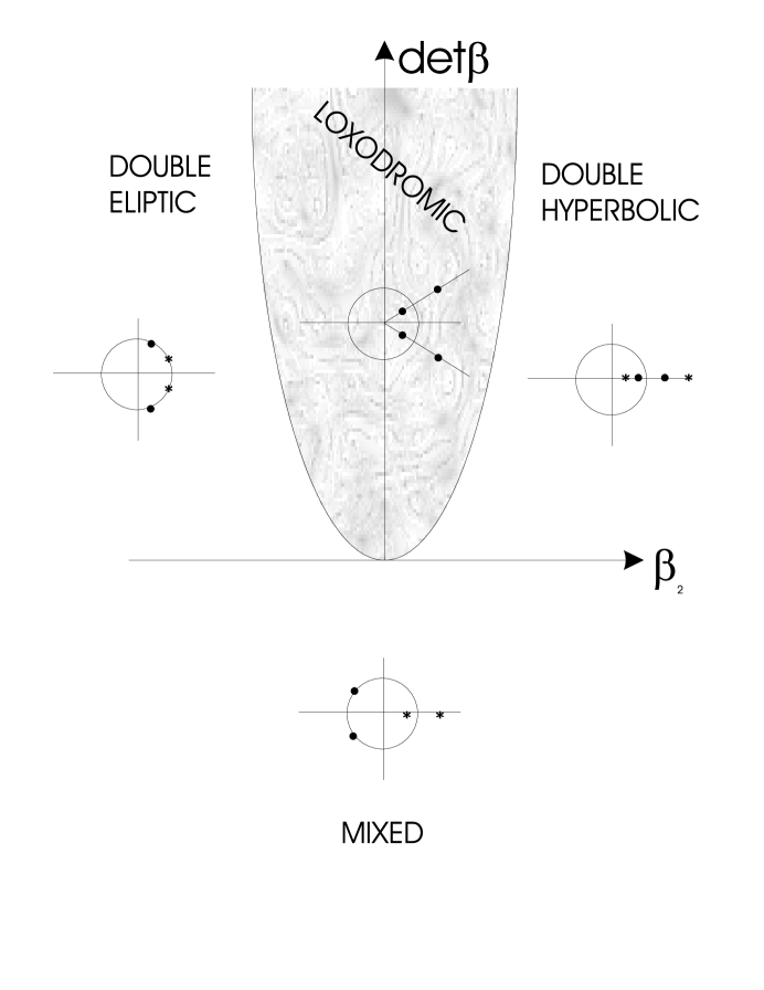
Figure 3.1: A classification of the different cat maps for two degrees of freedom according to the feline invariants of the ${\mathfrak{J}}\beta$ matrix. The parabolic boundary is $\det\beta=\left(\frac{\beta_{2}}{4}\right)^{2}.$ A similar picture exist for the ${\mathfrak{J}}B$ matrix.

Examples

We here show some examples of different types of cat maps. The examples are such that the $\beta$ matrix, that denotes the chord representation, has integer elements.

The Hannay and Berry Cat

It is important to see that the first cat map to be quantized ( the Hannay and Berry cat map) [7] can also be treated with the formalism described here . For a $2\times 2$ matrix, the characteristic polynomial reads,

$$P_{{\mathfrak{J}}\beta}(\lambda)=\lambda^{2}-\frac{1}{2}\beta_{2}.$$ (3.83)

For the symplectic matrix

$${\cal M}_{hb}=\left[\begin{array}[]{cc}2&1\\ 3&2\end{array}\right]\mbox{, with the associated symmetric matrix }\beta_{hb}=\left[\begin{array}[]{cc}3&0\\ 0&-1\end{array}\right],$$ (3.84)

so that

$$\beta_{2}=Tr\left[\left({\mathfrak{J}}\beta_{hb}\right)^{2}\right]=6,$$

the number of fixed points is

$$\tau_{\xi}^{hb}=\left|\frac{2^{2}}{P_{{\mathfrak{J}}\beta}(\lambda)}\right|=2$$

and the eigenvalues of the matrix ${\cal M}_{hb}$ are

$$\lambda_{1}^{hb} = 2+\sqrt{3}$$

$$\lambda_{2}^{hb} = 2-\sqrt{3}.$$

The map is then hyperbolic.

The double hyperbolic case

Let us now study cat maps that have two pairs of eigenvalues both in the real axis, that is, maps belonging to the first quadrant in figure 3.1. The $\beta_{hh}\,$ matrix below describes this case, the associated symplectic matrix being ${\cal M}_{hh}$ :

$$\beta_{hh}=\left[\begin{array}[]{cccc}0&2&1&2\\ 2&0&2&1\\ 1&2&0&0\\ 2&1&0&1\end{array}\right]\quad\mbox{and }\quad{\cal M}_{hh}=\left[\begin{array}[]{cccc}2&-2&-1&0\\ -2&3&1&0\\ -1&2&2&1\\ 2&-2&0&1\end{array}\right].$$ (3.85)

The invariants are

$$\det\beta_{hh}=17\quad\mbox{and }\quad\beta_{2}=Tr\left[\left({\mathfrak{J}}\beta_{hh}\right)^{2}\right]=20.$$

Thus, the number of fixed points $\tau_{\xi}^{hh}=2$ and the eigenvalues of the symplectic matrix ${\cal M}$ are

$$\lambda_{1}^{hh} = 2.112388$$

$$\lambda_{2}^{hh} = 0.4739$$

$$\lambda_{3}^{hh} = 5.22$$

$$\lambda_{4}^{hh} = 0.1914.$$

The mixed case

We consider here the case where the eigenvalues of the map are of mixed nature, i.e. there is a couple of real eigenvalues and a complex conjugated pair on the unit circle. This corresponds to $\beta$ matrices that belong to the third and fourth quadrant in figure  3.1.

One matrix of this kind is $\beta_{eh1}$, the associated symplectic matrix being ${\cal M}_{eh1}:$

$$\beta_{eh1}=\left[\begin{array}[]{cccc}0&2&1&2\\ 2&0&2&1\\ 1&2&0&2\\ 2&1&2&0\end{array}\right]\quad\mbox{and }\quad{\cal M}_{eh1}=\left[\begin{array}[]{cccc}0&0&-1&0\\ 0&0&0&-1\\ 1&0&2&1\\ 0&1&1&2\end{array}\right].$$ (3.86)

The invariants are

$$\det\beta_{eh1}=-15\quad\mbox{and }\quad\beta_{2}=Tr\left[\left({\mathfrak{J}}\beta_{eh1}\right)^{2}\right]=4.$$

Thus, the number of fixed points $\tau_{\xi}^{eh1}=1$ and the eigenvalues of the symplectic matrix ${\cal M}$ are

$$\lambda_{1}^{eh1} = 2.6180$$

$$\lambda_{2}^{eh1} = 0.381966$$

$$\lambda_{3}^{eh1} = \exp\left(i\frac{2\pi}{6}\right)$$

$$\lambda_{4}^{eh1} = \exp\left(-i\frac{2\pi}{6}\right).$$

This example shows rotation angles that are fractional multiples of $\pi$, for which the dynamics are equivalent to that of hyperbolic systems with one degree of freedom . Another example of a mixed system is given by the matrix $\beta_{eh2}$, the associated symplectic matrix being ${\cal M}_{eh2}:$

$$\beta_{eh2}=\left[\begin{array}[]{cccc}0&2&1&2\\ 2&0&2&1\\ 1&2&0&2\\ 2&1&2&1\end{array}\right]\quad\mbox{and }\quad{\cal M}_{eh2}=\left[\begin{array}[]{cccc}0&0&-1&0\\ 0&-1&-1&-2\\ 1&0&2&1\\ 0&2&2&3\end{array}\right].$$ (3.87)

Now we have

$$\det\beta_{eh2}=-7\quad\mbox{and }\quad\beta_{2}=Tr\left[\left({\mathfrak{J}}\beta_{eh2}\right)^{2}\right]=4.$$ (3.88)

Thus, the number of fixed points $\tau_{\xi}^{eh2}=2$ and the eigenvalues of the symplectic matrix ${\cal M}$ are

$$\lambda_{1}^{eh2} = 3.0906578$$

$$\lambda_{2}^{eh2} = 0.32355571$$

$$\lambda_{3}^{eh2} = \exp\left(i1.27354496\right)$$

$$\lambda_{4}^{eh2} = \exp\left(-i1.27354496\right).$$

In this example there are no rotations with angles that are a fraction of $\pi,$ the dynamics will then be ergodic and mixing in the whole phase space.

The loxodromic case

We choose now a $\beta$ matrix that belongs to the loxodromic region in Fig  3.1, for example $\beta_{lox}$, whose associated symplectic matrix being ${\cal M}_{eh1}:$

$$\beta_{lox}=\left[\begin{array}[]{cccc}0&2&1&0\\ 2&0&2&1\\ 1&2&1&1\\ 0&1&1&1\end{array}\right]\quad\mbox{and }\quad{\cal M}_{lox}=\left[\begin{array}[]{cccc}0&1&0&0\\ 0&1&1&0\\ 1&-1&1&1\\ -1&-1&-2&0\end{array}\right]$$ (3.89)

whose invariants are

$$\det\beta_{lox}=5\quad\mbox{and }\quad\beta_{2}=Tr\left[\left({\mathfrak{J}}\beta_{lox}\right)^{2}\right]=-4.$$

Thus, the number of fixed points $\tau_{\xi}^{lox}=2$ and the eigenvalues of the symplectic matrix ${\cal M}$ are

$$\lambda_{1}^{lox} = 1.7000157\exp\left(i1.1185178\right)$$

$$\lambda_{2}^{lox} = 1.7000157\exp\left(-i1.1185178\right)$$

$$\lambda_{3}^{lox} = 0.5882298\exp\left(i1.1185178\right)$$

$$\lambda_{4}^{lox} = 0.5882298\exp\left(-i1.1185178\right).$$

There are no rational rotations, so the dynamics is ergodic and mixing in the whole phase space.

The double elliptic case

In this case, the eigenvalues are characterized by two rotation angles. An interesting feature is that the condition that the ${\cal M}$ matrix have integer elements, prevents either angle from being an irrational multiple of $\pi.$ This restricts the dynamics to the trivial integrability observed for one degree of freedom systems.

In conclusion, any symplectomorphism on the $4$-torus belongs to one of the following cases:

1. Ergodic on the full phase space (a manifold of 2 degrees of freedom). For the double hyperbolic, mixed or loxodromic cases with irrational rotation angles.

2. Ergodic in a $2$-dimensional manifold . We have a constant of the motion, then the ergodicity is restricted to a low dimensional manifold (a manifold with $L=1).$ For the mixed or loxodromic cases with rational rotation angles.

3. A root of unity: that is, we have two constants of the motion. All orbits are periodic and have the same period for this double elliptic cases.

4 Simple Quantum Cat maps

Quantum dynamics is characterized by a unitary evolution operator, or propagator. It is possible to obtain the center and chord representation of an operator on the torus from its counterpart on the plane. This will be the way that we quantize cat maps, leaving the general construction for the next section. In some cases the quantum propagator denoting cat maps in the center or chord representation acquires simple expressions; in this section we will treat these special cases. More details about torus Hilbert space and its center and chord representations based on reference [8] are available in Appendix A.

It is well known that torus quantization implies that the Hilbert space $\left[{\cal H}_{N}^{\chi}\right]^{L}$ associated to the $2L$-torus has finite dimension $N^{L}$ and is characterized by a vector Floquet parameter $\chi=(\chi_{p},\chi_{q})$ whose components are real numbers belonging to $\left[0,1\right].$ The fact that $\left[{\cal H}_{N}^{\chi}\right]^{L}$ has finite dimension, implies that position and momentum eigenstates can only take on a set of discrete values that form a discrete lattice called quantum phase space (QPS). Any point $x$ in this QPS has coordinates,

$$x=\left(\begin{array}[]{c}p_{m}\\ q_{n}\end{array}\right)=\frac{1}{N}\left(\begin{array}[]{c}m+\chi_{p}\\ n+\chi_{q}\end{array}\right).$$ (4.1)

The center and chord representations are based on translation and reflection operators on this QPS as we show in [8]. Chords are of the form

$$\xi_{r,s}=\frac{1}{N}\left(\begin{array}[]{c}r\\ s\end{array}\right)=\frac{1}{N}\bar{\xi},$$ (4.2)

with $r$ and $s$ integer numbers and $\bar{\xi}=\left(\begin{array}[]{c}r\\ s\end{array}\right)$, while the center points $x_{a,b}$ are labeled by half-integer numbers $a$ and $b,$

$$x_{a,b}=\frac{1}{N}\left(\begin{array}[]{c}a+\chi_{p}\\ b+\chi_{q}\end{array}\right).$$ (4.3)

At a first stage we restrict our attention to those maps that can be quantized on the Floquet parameters $\chi=(0,0).$ As we will see in section 5 this implies that the matrix ${\cal M}$ must satisfy

$$\sum_{j=1}^{L}{\cal M}_{i,j}{\cal M}_{i,j+L}=\mbox{even integer for all }i.$$ (4.4)

As we will show in section 5, if $2\tau_{\xi}^{\prime}$, defined in (2.59), and $N$ are coprime numbers, a complete representation of the propagator is obtained having the symbol on a lattice of chords $\Xi$ such that

$$\Xi=\xi+{\bf n=}\frac{2\tau_{\xi}^{\prime}}{N}\overline{\Xi},$$ (4.5)

where the components of $\overline{\Xi}$ are integer numbers up to $N.$ So for any chord $\xi$ there is an equivalent chord $\Xi.$ For the allowed values of $N$, the propagator for cat maps in the chord representation takes the form

$${\bf U}_{\cal M}(\Xi)=2^{L}\left(\tau_{\xi}\right)^{-\frac{3}{2}}e^{-i2\pi N\left[\frac{1}{4}\Xi\beta\Xi\right]}\sum_{{\bf m\in\Diamond}_{\xi}}e^{-i2\pi N\frac{1}{4}{\bf m}(\beta-\widetilde{{\mathfrak{J}}}){\bf m}},$$ (4.6)

where $\tau_{\xi}$ is the number of fixed points of the classical map. For $\beta$ matrices that fulfill the feline conditions, the symbol ${\bf U}_{\cal M}^{0}(\Xi)$ must represent an unitary operator. In that case (A.43) shows that it must has the form

$${\bf U}_{\cal M}(\Xi)=\frac{e^{i\varphi_{N}({\cal M})}}{\sqrt{N}^{L}}e^{-i2\pi N\left[\frac{1}{4}\Xi\beta\Xi\right]},$$ (4.7)

which restricts

$$\frac{e^{i\varphi_{N}({\cal M})}}{\sqrt{N}^{L}}=2^{L}\left(\tau_{\xi}\right)^{-\frac{3}{2}}\sum_{{\bf m\in\Diamond}_{\xi}}e^{-i2\pi N\frac{1}{4}{\bf m}(\beta-\widetilde{{\mathfrak{J}}}){\bf m}}.$$ (4.8)

At first sight, the phase $\varphi_{N}({\cal M})$ is only an unimportant global phase factor, but the interference of the different $\varphi_{N}({\cal M}^{l})$ for the different powers $l$ of the map will have a crucial importance for the density of states.

As $\xi$ and $\Xi$ are equivalent chords, the symbol ${\bf U}_{\cal M}(\xi)\,$ and ${\bf U}_{\cal M}(\Xi)$ are related by symmetry relations (A.35) so that

$${\bf U}_{\cal M}(\xi)=\frac{e^{i\varphi_{N}({\cal M})}}{\sqrt{N}^{L}}e^{-i2\pi N\left[S(\xi,{\bf n})\right]},$$ (4.9)

where $S(\xi,{\bf n})$ is the action of the classical orbit whose chord is $\xi$ and that performs ${\bf n}$ loops around the torus as defined in (2.37).

If we chose the symplectically invariant form (2.30) for the $\xi$-independent part of the chord generating function, instead of (2.33), we would have in (4.9) a supplementary phase factor $e^{i2\pi N\frac{1}{4}{\bf n}\widetilde{{\mathfrak{J}}}{\bf n}}=e^{i\gamma_{{\bf n}}}$ with $\gamma_{{\bf n}}$ a ”Maslov index” for the orbit. This observation is true for all the following quantum theory.

In the case of the center representation, for $2\tau_{x}^{\prime}\,,$ defined in (2.58), and $N$ coprime numbers, a complete representation of the propagator is obtained by performing a transformation to center points $X$ that are integer multiples of $\frac{\tau_{x}^{\prime}}{N}$,

$$X=x+\frac{1}{2}{\bf j=}\frac{\tau_{x}^{\prime}}{N}\overline{X},$$ (4.10)

where the components of $\overline{X}$ are integer numbers up to $N$ [8]. On these points the center representation of the propagator takes the form

$${\bf U}_{\cal M}(X) = 2^{L}\tau_{x}^{-\frac{3}{2}}e^{i2\pi N\left[XBX\right]}\sum_{{\bf m\in\Diamond}_{x}}e^{i2\pi N\frac{1}{4}{\bf m}(B+\widetilde{{\mathfrak{J}}}){\bf m}}$$ (4.11)

$$= e^{i\varphi_{N}^{\prime}({\cal M})}e^{i2\pi N\left[XBX\right]},$$ (4.12)

where the last equality is obtained by imposing the unitarity of ${\bf\hat{U}}_{\cal M}$ and using (A.44). Hence, we define the angle $\varphi_{N}^{\prime}({\cal M})$ so

$$e^{i\varphi_{N}^{\prime}({\cal M})}=2^{L}\tau_{x}^{-\frac{3}{2}}\sum_{{\bf m\in\Diamond}_{x}}e^{i2\pi N\frac{1}{4}{\bf m}(B+\widetilde{{\mathfrak{J}}}){\bf m}}.$$ (4.13)

From the symmetry relations (A.38), we find that the symbols on the original points $x$ are

$${\bf U}_{\cal M}(x)=e^{i\varphi_{N}^{\prime}({\cal M})}e^{i2\pi N\left[S(x,{\bf j})\right]},$$ (4.14)

where here $S(x,{\bf j})\,$ is the center generating function, defined in (2.36), on a center point $x$ for an orbit performing ${\bf j}$ loops. The cases above are then special cases where the propagator on the torus has the same form as its equivalent on the plane; thus, they are ideally suited for the comparison of classical and quantum motion.

To obtain the more familiar position representation of the propagator from its chord representation, we use (A.39),

$${\bf U}_{\cal M}{\bf(q}_{m},{\bf q}_{n})=\frac{e^{i\varphi_{N}({\cal M})}}{(N)^{\frac{3L}{2}}}\sum_{\xi_{p}=0}^{N-1}\exp\left\{-i2\pi N\left[S(\xi_{p,m-n},{\bf n)+}\frac{q_{m}+q_{n}}{2}\xi_{p}\right]\right\},$$ (4.15)

While (A.40) allows us to obtain the position representation from the center one:

$${\bf U}_{\cal M}{\bf(q}_{m},{\bf q}_{n})=\frac{e^{i\varphi_{N}^{\prime}({\cal M})}}{N^{L}}\sum_{x_{p}=0}^{\frac{N-1}{2}}\exp\left\{i2\pi N\left[S(x_{p,\frac{m+n}{2}},{\bf j)+}\left(q_{m}-q_{n}\right)x_{p}\right]\right\}.$$ (4.16)

For the case of one degree of freedom, this leads to the Hannay and Berry propagator.

As we will see in section 5, condition (4.4) is preserved for the different powers of the map, hence, if a map is quantizable on the Floquet parameters $\chi=(0,0),$ all its powers also are. Furthermore, the propagator for ${\cal M}^{l}$ has the form

$${\bf U}_{\cal M}(\Xi)=\frac{e^{i\varphi_{N}({\cal M})}}{\sqrt{N}^{L}}e^{-i2\pi N\left[\frac{1}{4}\Xi\beta^{(l)}\Xi\right]},$$ (4.17)

in the chord representation, where $\beta^{(l)}$ denotes the symmetric matrix associated to ${\cal M}^{l}$ through (2.21) and $\Xi$ are points on a lattice of the form

$$\Xi{\bf=}\frac{\tau({\cal M}^{l})}{N}\overline{\Xi}.$$ (4.18)

As we discussed in section 2, lattices of rational points are invariant under classical cat maps. The denominator $g$ of these rational points can then be used to label the lattice, i.e. there exists a minimal period $l_{g}$ under which all the points on the lattice are fixed for ${\cal M}^{l_{g}}.\,$In other words, ${\cal M}^{l_{g}},$ restricted to the mentioned lattice, is the identity. We will call $l_{g}$ the classical periodicity function of the lattice. As we can see in the appendix, torus quantization is performed on a lattice of rational points whose denominator is $N$. Under these considerations we find that the quantum propagator is also periodic.

It is now possible to define conditions on the matrix ${\cal M}$ and the dimension of the Hilbert space $N\,$ under which $\widehat{{\bf U}}_{\cal M}\,$ reduces to the identity operator, i.e.

$$\widehat{{\bf U}}_{\cal M}=\widehat{{\bf 1}}_{N}e^{i\phi}.$$ (4.19)

This is best seen in the center representation, where we have (A.42)

$${\bf U}_{\cal M}(x)={\bf 1}_{N}(x)e^{i\phi}=e^{i\phi}f_{N}(x),$$ (4.20)

with $f_{N}(x)$ defined in (A.32). For the case where $N$ is an odd integer, we can perform the quantization on points $X$ that are integer multiples of $\frac{\tau_{x}^{\prime}}{N}$ , as we already discussed. We can see that if the $B$ matrix has all its elements that are multiples of $\frac{N}{\tau_{x}^{\prime}},$ then the propagator given by (4.11) has the form (4.20), where $f_{N}(X)=1$ and $\phi=\varphi_{N}^{\prime}({\cal M})$. Hence, the $B$ matrix denotes the identity if all its coefficients are multiples of $\frac{N}{\tau_{x}^{\prime}}.$ This implies through (2.25) that the ${\cal M}$ matrix must have the form

$${\cal M}={\bf 1\quad}\mbox{mod}(N),$$ (4.21)

in agreement with reference [7] for the $L=1$ case.

For any matrix ${\cal M}\,$ and for a given odd value of $N$, there is some smallest integer $k(N)$ such that

$${\cal M}^{k(N)}={\bf 1\quad}\mbox{mod}(N)$$ (4.22)

and in this way

$$\left[\widehat{{\bf U}}_{\cal M}^{0}\right]^{k(N)}={\bf 1}e^{i\phi(N)}.$$ (4.23)

In this sense, we may call the quantum propagator periodic with a period equal to $k(N)\,$ that we then call the quantum period function (QPF) although it is completely determined by the classical map through (4.22). Note that $k(N)=l_{N}$, i.e., the quantum and classical period function coincide for $N$ an odd number, as we would expect. It is now easy to see that the $N^{L}\,$ eigenangles $\theta_{m}$ of the unitary propagator $\widehat{{\bf U}}_{\cal M}$ are then restricted to lie on the $k(N)$ possible sites

$$\left\{\alpha_{j}=\left[\frac{2j\pi+\phi(N)}{k(N)}\right]\right\},1\leq j\leq k(N).$$ (4.24)

The eigenangle spectrum may be related to the traces of the propagator

$${\bf Tr}\left[\left(\widehat{{\bf U}}_{\cal M}\right)^{l}\right] = \sum_{m=1}^{N^{L}}e^{il\theta_{m}}$$ (4.25)

$$= \sum_{j=1}^{k(N)}d_{j}e^{il\alpha_{j}}$$ (4.26)

where $d_{j}$ is the degeneracy of the $j$th site defined by (4.24). The density of states,

$$\rho(\theta)=\sum_{i=l}^{N^{L}}\sum_{l=-\infty}^{\infty}\delta(\theta-\theta_{i}+2\pi l)$$ (4.27)

is clearly invariant under $\theta\rightarrow\theta+2\pi.$ Use the Poisson summation formula, leads to the trace formula,

$$\rho(\theta)=\frac{N^{L}}{2\pi}+\frac{1}{\pi}\mbox{Re}\sum_{l=1}^{\infty}{\bf Tr}\left[\left(\widehat{{\bf U}}_{\cal M}\right)^{l}\right]e^{-il\theta},$$ (4.28)

which holds for all maps on the $2L$-torus. Now, for the cat map, the fact that the propagator has periodicity $k(N)$ means that the density of states can also be written in the form [11]

$$\rho(\theta)=\sum_{l=1}^{k(N)}{\bf Tr}\left[\left(\widehat{{\bf U}}_{\cal M}\right)^{l}\right]e^{-il\theta}\sum_{j=-\infty}^{\infty}\delta(\phi(N)+2\pi j-k(N)\theta).$$ (4.29)

That is, the eigenangles are restricted to the sites $\alpha_{j}$ in (4.24), with the degeneracy at the $j$th site being given by

$$d_{j}=\frac{1}{k(N)}\sum_{l=1}^{k(N)}{\bf Tr}\left[\left(\widehat{{\bf U}}_{\cal M}\right)^{l}\right]e^{-il\alpha_{j}}.$$ (4.30)

This last equation then leads to simple expressions for several important properties of the eigenangle distribution; for example

$$\sum_{j=1}^{k(N)}d_{j}^{2}=\frac{1}{k(N)}\sum_{l=1}^{k(N)}\left|{\bf Tr}\left[\left(\widehat{{\bf U}}_{\cal M}\right)^{l}\right]\right|^{2}.$$ (4.31)

It is important to note that the $\delta$-functions appear explicitly in (4.29), because the propagator is periodic. The different powers of the quantum map in (4.29) contribute only to the finite degeneracies, not to the $\delta$-function form of the trace formula. Moreover, for all finite $N$, only a finite number of these powers are required to determine the degeneracy at every available site, and hence give the whole spectrum. However, $k(N)\rightarrow\infty$ as $N\rightarrow\infty$, thus more terms are required to determine the spectrum as the semiclassical limit is approached.

We now take the trace of (4.17), using (A.41), to obtain

$${\bf Tr}\left[\left(\widehat{{\bf U}}_{\cal M}\right)^{l}\right] = {\bf U}_{{\cal M}^{l}}(\xi=0)$$ (4.32)

$$= 2^{L}\left(\tau({\cal M}^{l})\right)^{-\frac{3}{2}}\sum_{{\bf m\in\Diamond}_{\xi}^{l}}\exp\left[-i2\pi N\frac{1}{4}{\bf m}(\beta^{(l)}-\widetilde{{\mathfrak{J}}}){\bf m}\right]=\frac{e^{i\varphi_{N}({\cal M}^{l})}}{\sqrt{N}^{L}},$$ (4.33)

where we recognize the action of the periodic orbits in the summation exponent, so

$${\bf Tr}\left[\left(\widehat{{\bf U}}_{\cal M}\right)^{l}\right] = 2^{L}\left|\det({\cal M}^{l}-1)\right|^{-\frac{3}{2}}\sum_{{\bf m\in\Diamond}_{\xi}^{l}}e^{-i2\pi N\left[S_{f}^{l}({\bf m})\right]}$$ (4.34)

$$= \frac{e^{i\varphi_{N}({\cal M}^{l})}}{\sqrt{N}^{L}}.$$ (4.35)

Note that ${\bf m\in\Diamond}_{\xi}^{l}$ implies that we are summing over the periodic orbits of period $l$. Equation (4.34) represents the Gutzwiller-Tabor trace formula [12] for the cat map, though we must note that, instead of being a semiclassical approximation, it is exact in this case. We must also note that the expression (4.35) for the traces of the propagator implies that in the expression (4.29) for the density of states, we have interference of the different phase factors $e^{i\varphi_{N}({\cal M}^{l})}$ for the different powers $l$ of the map.

Examples :

We will now study some quantum features of the classical examples studied in section 3. All of them fulfill condition (4.4), so that their symmetric $\beta$ matrix has integer entries. Then quantization can be performed for all odd values of $N,$ for which the quantum propagator will have the form

$${\bf U}_{\cal M}(\Xi)=\sqrt{\frac{1}{N^{L}}}e^{-i2\pi N\left[\frac{1}{4}\Xi\beta\Xi\right]}$$ (4.36)

in the chord representation. In this case, the chords $\Xi$, defined in (5.70), form a lattice of spacing $\frac{2}{N}.$ In the following, we will study the quantum period function for these maps.

We take cat maps of two degrees of freedom already studied in section 2. These include all the possible classical behaviors and we will study their effect on the QPF defined in (4.22).

The Hannay and Berry cat map

To compare the different types of behavior that occur for two degrees of freedom, it is important to present the already known QPF for the Hannay and Berry cat map whose symplectic matrix is ${\cal M}_{hb}$ defined in (3.84). The QPF is shown in figure  4.2, where we can then see that, although it has an irregular behavior as a whole, most of the points lie in families of straight lines which admit a maximum slope. Indeed, this indicates that there exists an increasing sequence of primes $p$ such that $\frac{p}{k(p)}<C$ for some $C$ independent of $N.$ According to Degli Esposti et al [9], this implies that the quantum map is ergodic and mixing in the semiclassical limit, within the definition of Von Neumann [10]. The average behavior of the QPF was established by Keating [11] and it is shown that in the semiclassical limit ($N\rightarrow\infty$)

$$\left\langle\log\frac{k(N)}{N}\right\rangle\approx\frac{-2\sqrt{\pi}}{e^{2}}\left(\log\log N\right)\left(\log\log\log N\right)$$ (4.37)

that is, the degeneracy grows very slowly with $N.$

Figure 4.2: The QPF for the Hannay and Berry cat map, chaotic with one degree of freedom, whose symplectic matrix is ${\cal M}_{hb},$ defined in (3.84).

The double hyperbolic case

We now choose the symmetric matrix $\beta_{hh}\,$ whose associated symplectic matrix is given by ${\cal M}_{hh}$ defined in (3.85). The QPF of this map is shown in figure  4.3. As we can see, the behavior is very different of that obtained for the Hannay and Berry Cat map. There are now families of parabolas instead of straight lines. The role played by $N$ in figure  4.2 is here played by $N^{2}$, because there are here $N^{2}$ states for this system. We conjecture that this kind of behavior implies quantal ergodicity and mixing for two degrees of freedom systems in the semiclassical limit, although a more formal study of this conjecture will be realized in a future work.

Figure 4.3: The QPF for the double hyperbolic map, whose symplectic matrix is ${\cal M}_{hh},$ defined in (3.85).

The mixed case

We first consider the map whose symmetric matrix is $\beta_{eh1},$ defined in (3.86), whose QPF is shown in figure  4.4. This is compared to $\beta_{eh2}$, defined in (3.87), characterized by irrational rotation angles, whose QPF is now shown in figure  4.5. There is a marked difference in the behavior between figure  4.4. and figure  4.5. While the former is very similar to the one obtained in figure  4.2 for a chaotic one degree of freedom system, the one of figure  4.5. is close to figure  4.3. for a system of two degrees of freedom. The very different behavior, as was explained in section 3, is due to the fact that the classical eigenvalues $\lambda_{3}^{eh1}$ and $\lambda_{4}^{eh1}$ denote rotation by angles that are a fraction of $\pi.$ Then the behavior of the system will be equivalent a hyperbolic system with a single degree of freedom and it is ergodic only in a subspace. On the contrary, $\lambda_{3}^{eh2}$ and $\lambda_{4}^{eh2}$ denote rotation angles that are irrational fractions of $\pi,$ so that classical and semiclassically the ergodicity appears in the whole phase space.

Figure 4.4: The QPF for the mixed map , with rational rotations, whose symplectic matrix is ${\cal M}_{eh1},$ defined in (3.86).

Figure 4.5: The QPF for the mixed map, with irrational rotations, whose symplectic matrix is ${\cal M}_{eh2},$ defined in (3.87) .

The loxodromic case

Let us now study the map denoted by the $\beta_{lox}$ matrix defined by (3.89). The corresponding QPF is shown in figure  4.6. The behavior is then similar to the one obtained for ergodic systems with two degrees of freedom. This map then manifests classical and semiclassical ergodicity on the whole phase space or the corresponding Hilbert space. Similarly to the previous example, we found that rotation angles that are a fraction of $\pi$ behave similarly to hyperbolic one degree of freedom maps shown in figure  4.5.

Figure 4.6: The QPF for the double loxodromic map of two degrees of freedom, with irrational rotations, whose symplectic matrix is ${\cal M}_{lox},$ defined in (3.89).

5 The quantum feline group

In this section we present the general quantization of multidimensional cat maps constructed in section two. In a first step we establish the conditions for the maps to be quantizable and then we construct their center and chord representations, based on the formalism developed in reference [8] and summarized in the Appendix.

The classical automorphism generated by ${\cal M}\,$ in plane phase space being linear, its quantization on the Hilbert space $\left[{\cal{H}_{{\mathbb{R}}}}\right]^{L}$ ,associated to the Euclidean phase space, will have the crucial property that

$$\widehat{U}_{\cal M}\widehat{T}_{\xi}\widehat{U}_{\cal M}^{\dagger}=\widehat{T}_{{\cal M}\xi}$$ (5.38)

for any translation operator $\widehat{T}_{\xi}$. We now show how to associate to any $\widehat{U}_{\cal M}$ a unitary operator on $\left[{\cal H}_{N}^{\chi}\right]^{L}$, the torus Hilbert space characterized by the Floquet parameter $\chi.$ For this purpose let us study the restriction of $\widehat{U}_{\cal M}$ to $\left[{\cal H}_{N}^{\chi}\right]^{L}.$ We then have:

Proposition

$$\widehat{U}_{\cal M}\left[{\cal H}_{N}^{\chi}\right]^{L}\subset\left[{\cal H}_{N}^{\chi^{\prime}}\right]^{L}$$ (5.39)

where

$$\chi^{\prime}={\cal M}\chi-\frac{N}{2}{\mathfrak{J}}\left({\cal M}\otimes{\cal M}\right)\quad\mbox{mod(1)}$$ (5.40)

where we have defined the vector product of two matrices as the vector whose components are

$$\left(A\otimes B\right)_{i}=\sum_{j=1}^{L}A_{i,j}B_{i,j+L}$$ (5.41)

Proof: Equation (5.38) implies

$$\widehat{U}_{\cal M}\widehat{T}_{\xi}=\widehat{T}_{{\cal M}\xi}\widehat{U}_{\cal M}.$$ (5.42)

We now restrict considerations to chords that perform integer loops around the torus, $\xi={\bf m,}$ with ${\bf m\,\,}$ an integer vector with $2L$ components,i.e., chords that generate translations that are equivalent to the identity on the torus. We thus act on a given state of $\left[{\cal H}_{N}^{\chi}\right]^{L}$ on each side of (5.42), so that inserting (A.20), we obtain

$$e^{\left[i2\pi N\left(\frac{1}{4}{\bf m}\widetilde{{\mathfrak{J}}}{\bf m}+{\bf m}\wedge\frac{\chi}{N}\right)\right]}\widehat{U}_{\cal M}|{\bf\Psi}>=e^{\left[i2\pi N\left(\frac{1}{4}{\bf m}{\cal M}^{t}\widetilde{{\mathfrak{J}}}{\cal M}{\bf m}+{\cal M}{\bf m}\wedge\frac{\chi^{\prime}}{N}\right)\right]}\widehat{U}_{\cal M}|{\bf\Psi}>,$$ (5.43)

for any vector ${\bf m}$. Now we chose ${\bf n}={\cal M}{\bf m}$ , hence, we find that

$${\bf n}\wedge\chi^{\prime}={\cal M}^{-1}{\bf n}\wedge\chi+\frac{N}{4}{\bf n}\left[\left({\cal M}^{-1}\right)^{t}\widetilde{{\mathfrak{J}}}\left({\cal M}^{-1}\right)-\widetilde{{\mathfrak{J}}}\right]{\bf n}\qquad\mbox{mod}(1)$$ (5.44)

and we specify $2L\,$independent integer vectors ${\bf n}\,=e_{j}\,(j=1,...,2L),$ such that each of them denotes one loop around one of the $j$-irreducible circuit on the torus. In this case $e_{j}\widetilde{{\mathfrak{J}}}e_{j}=0,$ using the symplectic property of ${\cal M}$ (2.3), and the fact that ${\mathfrak{J}}\widetilde{{\mathfrak{J}}}{\mathfrak{J}}=\widetilde{{\mathfrak{J}}}$, we obtain

$$e_{j}\wedge\chi^{\prime}={\cal M}^{-1}e_{j}\wedge\chi+\frac{N}{4}e_{j}{\mathfrak{J}}{\cal M}\widetilde{{\mathfrak{J}}}{\cal M}^{t}{\mathfrak{J}}e_{j}\mbox{mod(1)}.$$ (5.45)

Remarking that

$$\frac{N}{4}\left({\mathfrak{J}}{\cal M}\widetilde{{\mathfrak{J}}}{\cal M}^{t}{\mathfrak{J}}\right)_{i}=-\frac{N}{2}\sum_{j=1}^{L}{\cal M}_{i,j}{\cal M}_{i,j+L},$$ (5.46)

we finally obtain (5.40) after straightforward manipulations.

In the case $L=1$, (5.40) reduces to the already known result [9],[13],

$$\chi^{\prime}={\cal M}\chi-\frac{N}{2}{\mathfrak{J}}\left(\begin{array}[]{l}{\cal M}_{11}{\cal M}_{12}\\ {\cal M}_{21}{\cal M}_{22}\end{array}\right)\quad\mbox{mod(1)}.$$ (5.47)

For two degrees of freedom ($L=2$) we obtain:

$$\chi^{\prime}={\cal M}\chi-\frac{N}{2}{\mathfrak{J}}\left(\begin{array}[]{l}{\cal M}_{11}{\cal M}_{13}+{\cal M}_{12}{\cal M}_{14}\\ {\cal M}_{21}{\cal M}_{23}+{\cal M}_{11}{\cal M}_{24}\\ {\cal M}_{31}{\cal M}_{33}+{\cal M}_{32}{\cal M}_{34}\\ {\cal M}_{41}{\cal M}_{43}+{\cal M}_{42}{\cal M}_{44}\end{array}\right)\quad\mbox{mod(1)}.$$ (5.48)

Given ${\cal M},$ there exists for each $N$ a set of solutions of (5.40) such that $\chi^{\prime}=\chi$. This Floquet set of parameters is determined by

$$\chi=\frac{N}{2}\left({\cal M}-1\right)^{-1}{\bf i}_{\cal M}+\left({\cal M}-1\right)^{-1}{\bf m,}$$ (5.49)

where ${\bf i}_{\cal M}={\mathfrak{J}}\left({\cal M}\otimes{\cal M}\right)\mbox{mod(4)}\,$ is an integer vector. For this set of parameters the propagator $\widehat{U}_{\cal M}$ is such that

$$\left[\widehat{U}_{\cal M},\widehat{{\bf 1}}_{N}^{\chi}\right]=0,$$ (5.50)

where $\widehat{{\bf 1}}_{N}^{\chi}$ is the unit operator in $\left[{\cal H}_{N}^{\chi}\right]^{L}$ defined in (A.7). Evidently we cannot change the Floquet parameters at each iteration of the map, so (5.49) defines the quantizability set of the map. For this set of parameters, we can then restrict the unitary operators $\widehat{U}_{\cal M}\,$ to the Hilbert space of the $2L$-torus $\left[{\cal H}_{N}^{\chi}\right]^{L}$ and thus define the corresponding torus propagator as

$$\widehat{{\bf U}}_{\cal M}^{\chi}=\widehat{U}_{\cal M}\widehat{{\bf 1}}_{N}^{\chi}=\widehat{{\bf 1}}_{N}^{\chi}\widehat{U}_{\cal M}\widehat{{\bf 1}}_{N}^{\chi}.$$ (5.51)

Operators defined through (5.51) inherit the unitary from their plane counterpart and we will call them quantum cat maps.

The fact that the quantum symplectic map commutes with projections on the torus (A.17) leads to;

$$\widehat{{\bf U}}_{{\cal M}^{l}}^{\chi}=\left[\widehat{{\bf U}}_{\cal M}^{\chi}\right]^{l}.$$ (5.52)

The unitarity of $\widehat{{\bf U}}_{\cal M}^{\chi}$ and (5.52) implies that

$$\widehat{{\bf U}}_{\cal M}^{\chi}=\left[\widehat{{\bf U}}_{\cal M}^{\chi}\right]^{-1}=\left[\widehat{{\bf U}}_{\cal M}^{\chi}\right]^{\dagger}.$$ (5.53)

Having two cat maps ${\cal M}_{A}$ and ${\cal M}_{B}$ that are quantizable on the same Floquet parameter $\chi,$ implies that (A.17)

$$\widehat{{\bf U}}_{{\cal M}_{A}}^{\chi}\widehat{{\bf U}}_{{\cal M}_{B}}^{\chi}=\widehat{{\bf U}}_{{\cal M}_{A}{\cal M}_{B}}^{\chi},$$ (5.54)

that is, the quantization of the composition of different cat maps is equivalent to the composition of the quantization of each map. This shows that quantum cat maps form a group, the quantum propagator preserving the classical composition laws. This feline quantum group is at the same time a projection onto the torus of the metaplectic group and a subgroup of the classical feline group. It then follows that, for any power $l$, the map ${\cal M}^{l}$ is also quantizable.

The quantizability set of the map can be made independent of $N$ if the inhomogeneous term in (5.40) vanishes. This will be the case for matrices ${\cal M}$, such that

$${\bf m}\left({\cal M}^{t}\widetilde{{\mathfrak{J}}}{\cal M}\pm\widetilde{{\mathfrak{J}}}\right){\bf m=}0\qquad\mbox{mod}(2)$$ (5.55)

for any integer vector ${\bf m.}$ This condition is equivalent to

$$\sum_{j=1}^{L}{\cal M}_{i,j}{\cal M}_{i,j+L}=\mbox{even},$$ (5.56)

so that the allowed Floquet parameters are

$$\chi=\left({\cal M}-1\right)^{-1}{\bf m.}$$ (5.57)

In conclusion, the Floquet parameters are then denoted by the fixed points of the map (3.63). The QPS can thus have any of the fixed points of the map as its origin; without loss of generality, one can take $\chi=0.$ For the one degree of freedom case (5.56) implies that the ${\cal M}$ matrix must be restricted to the family of maps

$$\left(\begin{array}[]{cc}\mbox{even}&\mbox{odd}\\ \mbox{odd}&\mbox{even}\end{array}\right)\qquad\mbox{or\qquad}\left(\begin{array}[]{cc}\mbox{odd}&\mbox{even}\\ \mbox{even}&\mbox{odd}\end{array}\right)$$

selected as quantizable by Hannay and Berry [7].

Let us now provide an explicit construction of quantum cat maps based on the center and chord representations of operators. We start with the quantization of the linear automorphism ${\cal M}$ on the Hilbert space $\left[{\cal{H}_{{\mathbb{R}}}}\right]^{L}$ associated to the Euclidean phase space. The linearity of the ${\cal M}$ map implies in the exactness of the Van Vleck construction of the propagator [14]. This propagator in the chord representation has the form [4]

$$U_{\cal M}(\xi)=\left|\det\left[1\pm{\mathfrak{J}}\frac{\partial^{2}S(\xi)}{\partial\xi^{2}}\right]\right|^{\frac{1}{2}}e^{-\frac{i}{\hbar}S(\xi)}$$ (5.58)

where $S(\xi)\equiv S(\xi,0)$ is the chord generating function of the automorphism in the plane phase space. In the center representation, the Van Vleck propagator is

$$U_{\cal M}(x)=\left|\det\left[1\pm{\mathfrak{J}}\frac{\partial^{2}S(x)}{\partial x^{2}}\right]\right|^{\frac{1}{2}}e^{\frac{i}{\hbar}S(x)},$$ (5.59)

where now $S(x)\equiv S(x,0)$ is the center generating function of the transformation in the plane. Inserting (2.37) and (2.36) for the respective generating functions, we have [4]

$$U_{\cal M}(x)=\left|\det\left(1\pm{\mathfrak{J}}B\right)\right|^{-\frac{1}{2}}e^{\frac{i}{\hbar}xBx}$$ (5.60)

and

$$U_{\cal M}(\xi)=\left|\det\left(1\pm{\mathfrak{J}}\beta\right)\right|^{-\frac{1}{2}}e^{-\frac{i}{\hbar}\frac{1}{4}\xi\beta\xi}.$$ (5.61)

We may now project these representations on the $2L$-torus. For this purpose we must restrict our construction to the quantizability set of Floquet parameter $\chi$ defined through (5.49) and take the chord and center symbols of the projected operator. This is performed substituting (5.61) and (5.60) respectively in (A.45) and (A.46). Then we obtain the chord representation of the quantum cat map as an average over winding vectors:

$${\bf U}_{\cal M}^{\chi}(\xi)=\left|\det\left(1\pm{\mathfrak{J}}\beta\right)\right|^{-\frac{1}{2}}\left\langle e^{-i2\pi N\left[\frac{1}{4}\xi\beta\xi+\frac{1}{2}\xi(\beta+{\mathfrak{J}}){\bf m}+\frac{1}{4}{\bf m}(\beta-\widetilde{{\mathfrak{J}}}){\bf m+}\frac{\chi}{N}\wedge{\bf m}\right]}\right\rangle_{{\bf m}}.$$ (5.62)

There are various classical objects present in this formula. Recalling section 2, $S(\xi,{\bf m}),$ the chord generating function of the cat map defined in (2.37) appears in the exponent of (5.62). In the amplitude we recognize $\tau_{\xi},$ the number of fixed points of the map defined in (2.54), so that,

$${\bf U}_{\cal M}^{\chi}(\xi)=2^{L}\frac{1}{\sqrt{\tau_{\xi}}}\left\langle e^{-i2\pi N\left[S(\xi,{\bf m}){\bf+}\frac{\chi}{N}\wedge{\bf m}\right]}\right\rangle_{{\bf m}}.$$ (5.63)

Similarly, for the center representation we obtain

$${\bf U}_{\cal M}^{\chi}(x)=\left|\det\left(1\pm{\mathfrak{J}}B\right)\right|^{-\frac{1}{2}}\left\langle e^{i2\pi N\left[xBx+x(B-{\mathfrak{J}}){\bf m}+\frac{1}{4}{\bf m}(B+\widetilde{{\mathfrak{J}}}){\bf m-}\frac{\chi}{N}\wedge{\bf m}\right]}\right\rangle_{{\bf m}},$$ (5.64)

where we recognize $S(x,{\bf m}),$ the center generating function of the cat map (2.36), and $\tau_{x},$ the number of orbits centered on $x$ defined by (2.55), so that

$${\bf U}_{\cal M}^{\chi}(x)=2^{L}\frac{1}{\sqrt{\tau_{x}}}\left\langle e^{i2\pi N\left[S(x,{\bf m}){\bf-}\frac{\chi}{N}\wedge{\bf m}\right]}\right\rangle_{{\bf m}}.$$ (5.65)

Both (5.63) and (5.65) are representations of quantum cat maps of general dimension, showing that the quantum propagator is entirely defined in terms of classical objects, except for the term $\frac{\chi}{N}\wedge{\bf m}$ in the exponent that denotes the quantum features of the boundary conditions. However, we have to perform the average on ${\bf m}$ to make the representation explicit. Given that the quantizability set (5.49) only admits rational values of $\chi$, (5.63) and (5.65) are Gaussian sums. The quantizability condition (5.55) for the map ${\cal M}$ is equivalent to the condition that the Gaussian sums do not vanish for $L=1.$ We do not know of a similar verification for $L>1.$

In the following we will restrict our attention to maps that fulfill the condition (5.55), such that the inhomogeneous term in (5.40) vanishes. As we have already discussed, we can then choose $\chi=0$ without loss of generality. The quantum cat maps associated with these Floquet parameters will be denoted by $\widehat{{\bf U}}_{\cal M}$. All the examples in section 4 are of this type.

We now use the periodicity properties (2.44) of $S(\xi,{\bf m})$ to show that the exponential function in (5.63) is periodic. Indeed, for ${\bf m}^{\prime}$ defined in (2.42) and the generating function $S(\xi,{\bf m}^{\prime})$ defined in (2.44) we have that

$$e^{-i2\pi N\left[S(\xi,{\bf m}^{\prime})\right]}=e^{-i2\pi N\left[S(\xi,{\bf m})\right]}e^{-i2\pi N\left[\xi\wedge{\bf k-}\frac{1}{2}{\bf m}\Gamma_{1}{\bf k-}\frac{1}{4}{\bf k}\Delta_{1}{\bf k}\right]},$$ (5.66)

where $\Gamma_{1}$ and $\Delta_{1}$ were respectively defined in (2.46) and (2.47). We can now see that $e^{-i2\pi N\left[\xi\wedge{\bf k}\right]}=1$ for any integer vector ${\bf k}$ and for maps that fulfill the condition (5.55) $e^{-i2\pi N\left[{\bf-}\frac{1}{2}{\bf m}\Gamma_{1}{\bf k-}\frac{1}{4}{\bf k}\Delta_{1}{\bf k}\right]}=1,$ hence

$$\exp\left[-i2\pi NS\left(\xi,{\bf m}+({\cal M}-1){\bf k}\right)\right]=\exp\left[-i2\pi NS(\xi,{\bf m})\right].$$ (5.67)

The average in (5.63) is then periodic, so that, we sum over one period and divide by the number of points in the period, to perform such an average. Hence, we must restrict ${\bf m}$ to the fundamental parallelogram $\Diamond_{\xi}$ defined in (2.51), where there are exactly $\tau_{\xi}$ points ${\bf m}$ with integer coordinates:

$${\bf U}_{\cal M}(\xi) = 2^{L}\left(\tau_{\xi}\right)^{-\frac{3}{2}}\sum_{{\bf m\in\Diamond}_{\xi}}e^{-i2\pi N\left[S(\xi,{\bf m})\right]}$$ (5.68)

$$= 2^{L}\left(\tau_{\xi}\right)^{-\frac{3}{2}}\sum_{{\bf m\in\Diamond}_{\xi}}e^{-i2\pi N\left[\frac{1}{4}\xi\beta\xi+\frac{1}{2}\xi(\beta+{\mathfrak{J}}){\bf m}+\frac{1}{4}{\bf m}(\beta-\widetilde{{\mathfrak{J}}}){\bf m}\right]}.$$

Since ${\bf m}$ belongs to $\Diamond_{\xi},$ the sum in (5.68) is the sum over the different classical orbits whose chord is $\xi$.

In a similar way, for the center representation the periodicity region is the parallelogram $\Diamond_{x}\,,$ defined in (2.53), that has exactly $\tau_{x}$ points ${\bf m}$ with integer coordinates (2.55), so that

$${\bf U}_{\cal M}(x) = 2^{L}\tau_{x}^{-\frac{3}{2}}\sum_{{\bf m\in\Diamond}_{x}}e^{i2\pi N\left[S(x,{\bf m})\right]}$$ (5.69)

$$= 2^{L}\tau_{x}^{-\frac{3}{2}}\sum_{{\bf m\in\Diamond}_{x}}e^{i2\pi N\left[xBx+x(B-{\mathfrak{J}}){\bf m}+\frac{1}{4}{\bf m}(B+\widetilde{{\mathfrak{J}}}){\bf m}\right]},$$

i.e. we are taking the sum on the different classical orbits centered in $x.$ The expressions (5.68) and (5.69) have exactly the form expected for the semiclassical approximation of the propagator in center and chord representations respectively [4],[8] but in this case they are exact instead of being a mere approximation.

For generic cat maps, (5.68) and (5.69) generate Gaussian sums, but in some cases important simplifications are possible. Let us start, once more, with the chord representation. We have already seen that the matrix $\beta$ has the form $\beta=\frac{\overline{\beta}^{\prime}}{\tau_{\xi}^{\prime}}$, where the barred matrix has integer elements. The simplest case is when the cat map is such that the associated $\beta\,$matrix itself has integer entries. Recalling that $\xi=\frac{1}{N}\overline{\xi}$, we will transform to an equivalent set of chords, for which the values for $\overline{\xi}$ are even multiples of $\tau_{\xi}^{\prime}$. So, for any chord $\xi$ there is an equivalent chord $\Xi,$ such that

$$\Xi=\xi+{\bf n}=\frac{2\tau_{\xi}^{\prime}}{N}\overline{\Xi},$$ (5.70)

where the components of $\overline{\Xi}$ are integer numbers up to $N$ and the components of ${\bf n}$ are integer up to $2\tau_{\xi}^{\prime}-1$. Equation (5.70) has solutions with the specified features for any $\xi,$ only if $N\,$ and $2\tau_{\xi}^{\prime}\,$ are coprime numbers. We will then restrict $N$ to be an odd integer. In this case, the chords $\Xi$ in (5.70) form a lattice with spacing $\frac{2\tau_{\xi}^{\prime}}{N}.$ A hypercube of side $2\tau_{\xi}^{\prime}$ has then $N^{L}\times N^{L}$ successive chords $\Xi$ that constitute a basis for translation operators. For the simplest case where the matrix $\beta$ has integer entries, the chords $\Xi\,$ form a lattice of length $2$ with spacing $\frac{2}{N}.$ Performing the transformation to chords $\Xi,$ we see that the term $e^{-i2\pi N\left[\frac{1}{2}\Xi(\beta+{\mathfrak{J}}){\bf m}\right]}=1,$ so there is then no $\Xi$-dependence in the propagator sum (5.68), leading to(4.6).

In the same way, the matrix $B$ in the center representation has the form $B=\frac{\overline{B}^{\prime}}{\tau_{x}^{\prime}}$ . Then we transform to center points $X$ that are integer multiples of $\frac{\tau_{x}^{\prime}}{N}$,

$$X=x+\frac{1}{2}{\bf j}=\frac{\tau_{x}^{\prime}}{N}\overline{X},$$ (5.71)

where the components of $\overline{X}$ are integer numbers up to $N$ and the components of ${\bf j}$ are integer up to $2\tau_{x}^{\prime}-1$. Again, solutions of (5.71) with the specified features will exist only if $N$ and $2\tau_{x}^{\prime}$ are coprime numbers. Thus, reflection operators on points $X$, that form a lattice with separation $\frac{\tau_{x}^{\prime}}{N}$ on a hypercube of side $\tau_{x}^{\prime},$ form a basis for the Hilbert space of the torus. For center points $X$ in (5.71) , the term $e^{i2\pi N\left[X(B-{\mathfrak{J}}){\bf m}\right]}=1,$ so the propagator (5.69) has the form (4.11).

The above are then special cases where the propagator on the torus has the same form as its equivalent on the plane. These cases are then ideal to study quantization, as we have seen in section 4.

We will now discuss the quantum effect of a similarity transformation of the form

$${\cal M}\rightarrow{\cal M}^{\prime}={\cal N}^{-1}{\cal M}{\cal N}.$$ (5.72)

As we have already discussed the matrices ${\cal M}^{\prime}$ and ${\cal M}$ represent the same map, but seen on a different frame of canonical coordinates. On the torus, we have to restrict both ${\cal M}$ and ${\cal N}$ to have integer elements so that the torus is mapped on itself. This restricts the symplectic similarity transformations to the feline transformations.

The main advantage of the chord and center representation in plane phase space is their symplectic invariance[4]. It is well known that linear classical canonical transformations $x^{\prime}={\cal N}x$ correspond to unitary transformations in $\left[{\cal{H}_{{\mathbb{R}}}}\right]^{L}$,

$$\widehat{A}\rightarrow\widehat{A}^{\prime}=\widehat{U}_{\cal N}\widehat{A}\widehat{U}_{\cal N}^{-1}.$$ (5.73)

The effect of such a unitary transformation on the chord and center representation is merely

$$A(x)\rightarrow A({\cal N}x)\quad\mbox{and}\quad A(\xi)\rightarrow A({\cal N}\xi).$$ (5.74)

Because of the commutation of operator products with projection from the plane to the torus, the effect of a similarity transformation $\widehat{{\bf A}}\rightarrow\widehat{{\bf U}}_{\cal N}^{\chi}\widehat{{\bf A}}\left[\widehat{{\bf U}}_{\cal N}^{\chi}\right]^{-1}$ performed by a quantized cat map on any operator $\widehat{{\bf A}}$ that commutes with $\widehat{{\bf 1}}_{\cal N}^{\chi}$ will be purely classical in the center or the chord representations:

$${\bf A}(x)\rightarrow{\bf A}({\cal N}x)\quad\mbox{and\quad}{\bf A}(\xi)\rightarrow{\bf A}({\cal N}\xi).$$ (5.75)

Thus the similarity transformation among quantum cat maps, reduces to the classical similarity transformation:

$$\widehat{{\bf U}}_{{\cal M}^{\prime}}^{\chi}=\widehat{{\bf U}}_{\cal N}^{\chi}\widehat{{\bf U}}_{\cal M}^{\chi}\left[\widehat{{\bf U}}_{\cal N}^{\chi}\right]^{-1},$$ (5.76)

so that,

$${\bf U}_{{\cal M}^{\prime}}(x)={\bf U}({\cal N}x)\quad\mbox{and\quad}{\bf U}_{{\cal M}^{\prime}}(\xi)={\bf U}({\cal N}\xi).$$ (5.77)

However, the quantum cat maps ${\cal M}^{\prime}$ and ${\cal M}$ must be quantized on the same Floquet parameters $\chi$. This imposes another restriction on the matrix ${\cal N}$ used to perform the similarity transformation, its quantizability set must include the Floquet parameter $\chi.$ That is ${\cal M}$ and ${\cal N}$ must belong the same quantum feline group.

For two quantum cat maps $\widehat{{\bf U}}_{{\cal M}^{\prime}}^{\chi}$ and $\widehat{{\bf U}}_{\cal M}^{\chi}$ related by (5.76) and for all power $l$ of the map we have

$$Tr\left[\left(\widehat{{\bf U}}_{{\cal M}^{\prime}}^{\chi}\right)^{l}\right] = Tr\left\{\left(\widehat{{\bf U}}_{\cal N}^{\chi}\widehat{{\bf U}}_{\cal M}^{\chi}\left[\widehat{{\bf U}}_{\cal N}^{\chi}\right]^{-1}\right)^{l}\right\}=Tr\left\{\left(\widehat{{\bf U}}_{\cal M}^{\chi}\right)^{l}\left[\widehat{{\bf U}}_{\cal N}^{\chi}\right]^{-l}\left(\widehat{{\bf U}}_{\cal N}^{\chi}\right)^{l}\right\}$$ (5.78)

$$= Tr\left[\left(\widehat{{\bf U}}_{\cal M}^{\chi}\right)^{l}\right].$$

We have seen in (4.28) that the density of states and hence the spectrum of the system is uniquely determined through the traces of the different powers of the map. Then, (5.78) shows that $\widehat{{\bf U}}_{{\cal M}^{\prime}}^{\chi}$ and $\widehat{{\bf U}}_{\cal M}^{\chi}$ related by (5.76) have the same quasi-energy spectrum.

We now show that the quantum period function is also invariant with respect to a feline similarity transformation, for the periodic case where we can chose the Floquet parameter $\chi=0$. Suppose that the QPF corresponding to $\widehat{{\bf U}}_{{\cal M}^{\prime}}^{\chi}$ and $\widehat{{\bf U}}_{\cal M}^{\chi}$ are respectively $k_{{\cal M}^{\prime}}(N)$ and $k_{\cal M}(N)$ , then

$$\left({\cal M}^{\prime}\right)^{k_{\cal M}(N)}=\left({\cal N}^{-1}{\cal M}{\cal N}\right)^{k_{\cal M}(N)}={\cal N}^{-1}\left({\cal M}\right)^{k_{\cal M}(N)}{\cal N}.$$ (5.79)

For all points $x$ belonging to the QPS, i.e., a lattice of spacing $\frac{1}{N}$ on the $2L$-torus $\Box,$ we have

$$\left({\cal M}^{\prime}\right)^{k_{\cal M}(N)}x={\cal N}^{-1}\left({\cal M}\right)^{k_{\cal M}(N)}{\cal N}x=x,$$ (5.80)

hence

$$\left({\cal M}^{\prime}\right)^{k_{\cal M}(N)}={\bf 1\quad}\mbox{mod}(N),$$ (5.81)

so that

$$k_{{\cal M}^{\prime}}(N)\leq k_{\cal M}(N).$$ (5.82)

In the same way, for all points $x$ belonging to the QPS

$$\left({\cal M}\right)^{k_{{\cal M}^{\prime}}(N)}x={\cal N}\left({\cal M}^{\prime}\right)^{k_{{\cal M}^{\prime}}(N)}{\cal N}^{-1}x=x,$$ (5.83)

hence

$$k_{\cal M}(N)\leq k_{{\cal M}^{\prime}}(N).$$ (5.84)

Therefore,

$$k_{{\cal M}^{\prime}}(N)=k_{\cal M}(N),$$ (5.85)

  that is, the QPF of both quantum maps $\widehat{{\bf U}}_{{\cal M}^{\prime}}^{\chi}$ and $\widehat{{\bf U}}_{\cal M}^{\chi}$ coincide.

6 Conclusions

In this work we have studied classical and quantum properties of multidimensional Cat maps. In a first step the classical study was performed using the symplectically invariant center and chord generating functions. They allow us to represent the symplectic matrix by a symmetric one. This is the basis for a complete classification of generic four dimensional cat maps. Clearly, the advantage of working with the appropriate generating functions will be even more pronounced for cat maps of higher dimension. Two degrees of freedom are sufficient to obtain all distinct types of dynamics. Loxodromic behavior appears as a new alternative with respect to usual cat maps with one degree of freedom.

The quantization of cat maps was performed using the recently developed Weyl representation and its conjugate chord representation. The semiclassical approximation is exact whatever the number of degrees of freedom or the characteristics of the cat map. The spectral properties show the same kind of ”pathologies ” observed for systems with one degree of freedom. Through the quantum periodicity function, we have indication of quantal ergodicity and mixing in the semiclassical limit for systems that present this classical property. We must note that this is one of the first times that loxodromic behavior is quantized [15].

According to Anosov’s theorem, all cases of fully ergodic classical maps are structurally stable, that is, a weak nonlinear perturbation leads to a map whose orbits are topologically equivalent to the original cat map. The possibility of quantizing such an Anosov map is in no way restricted to one degree of freedom. In this way, one can obtain continuous families of quantum torus maps, corresponding to fully chaotic classical maps for each type of map ( doubly hyperbolic, loxodromic, etc.). These nonlinear maps will probably avoid the spectral anomalies due to quantum periodicity, as was verified for the case of a single degree of freedom [16] ,[17].

Acknowledgments: We thanks helpful discussions with J.P. Keating, who provide us Greenman preprint, E. Pujals and G. Contreras who provide us Mañe’s work. We acknowledge financial support from Pronex-MCT and A.M.F.R. also thanks support from CLAF-CNPq. This work was partially supported by contracts ANPCYT PICT97-01015, CONICET PIP98-420 and EC-931005AR.

Appendix A The Weyl quantization on the Torus

In this appendix we develop the mathematical tools needed for the quantization of cat maps, based on our previous work on Weyl quantization on the torus [8].

A.1 The Hilbert space of the torus

In a first stage it is important to treat the specification of the Hilbert space of quantum states, or prequantization, independently from the dynamics of the system. That is, we treat the quantum kinematics, corresponding to the geometrical description of phase space at the classical level. Just to simplify the notation we limit the presentation for one degree of freedom systems, since the extension for $L\neq 1$ is trivial.

A complete description for prequantization must include Bloch boundary conditions :

$${\bf\Psi}(q+1) = e^{2\pi i\chi_{p}}{\bf\Psi}(q),$$ (A.1)

$${\bf\tilde{\Psi}}(p+1) = e^{-2\pi i\chi_{q}}{\bf\tilde{\Psi}}(p)$$ (A.2)

where

$${\bf\tilde{\Psi}}(p)=(2\pi\hbar)^{-1/2}\int e^{-ipq/\hbar}{\bf\Psi}(q)dq,$$ (A.3)

and $2\pi i\chi_{p}$ and $2\pi i\chi_{q}$ are fixed arbitrary Floquet angles; that is, the prequantization depends on the vector $\chi=(\chi_{p},\chi_{q})$ whose coordinates are in the range $0\leq\chi_{q},\chi_{q}<1$. Solutions to (A.1) and (A.2) with the connection (A.3) only exist if there is an integer $N$, so that [13]

$$\hbar=\frac{1}{2\pi N}.$$ (A.4)

Then the space of solutions spans a Hilbert space ${\cal H}_{N}^{\chi}$ having the finite dimension $N$. Two bases of ${\cal H}_{N}^{\chi}$ appear in analogy with the position and momentum eigenvectors, here denoted by, $|{\bf q}_{n}>$ and $|{\bf p}_{m}>$ with $n,m=0,1,\dots,N-1$. According to the Bloch type boundary conditions, we will then define the position state on the torus as an average over equivalent positions in the plane phase space:

$$|{\bf q}_{n}>=\left\langle|\frac{n+\chi_{q}}{N}+k>e^{2\pi ik\chi_{p}}\right\rangle_{k},$$ (A.5)

with the Hermitian structure

$$<{\bf q}_{m}|{\bf q}_{n}>_{N,\chi}=<{\bf q}_{m}|{\bf q}_{n}>=\delta_{m,n}^{(N)}e^{\frac{2\pi i}{N}(m-n)\chi_{p}},$$ (A.6)

The identity operator in ${\cal H}_{N}^{\chi}$ is obtained through

$$\widehat{{\bf 1}}_{N}^{\chi}=\sum_{m=0}^{N-1}|{\bf q}_{m}><{\bf q}_{m}|.$$ (A.7)

In analogy, the momentum eigenvectors

$$|{\bf p}_{m}>=\left\langle|\frac{m+\chi_{p}}{N}+k>e^{-2\pi ik\chi_{q}}\right\rangle_{k},$$ (A.8)

normalized such that

$$<{\bf p}_{m}|{\bf p}_{n}>=\delta_{m,n}^{(N)}e^{-\frac{2\pi i}{N}(m-n)\chi_{q}}.$$ (A.9)

The bases are exchanged with the transformation kernel,

$$<{\bf p}_{m}|{\bf q}_{n}>=N^{-1/2}e^{2\pi i(m+\chi_{p})(n+\chi_{q})/N}\equiv(F_{N}^{\chi})_{mn},$$ (A.10)

forming a unitary matrix (finite Fourier transformation). According to (A.4) the classical limit corresponds to $N\rightarrow\infty$ .

We then see that positions and momenta form a discrete web on the torus, that we will call from now on the quantum phase space QPS in accordance with [18]. For the case of $L$ degrees of freedom, the Hilbert space of the $2L$-torus is $\left[{\cal H}_{N}^{\chi}\right]^{L}={\cal H}_{N}^{\chi}\times{\cal H}_{N}^{\chi}\times...\times{\cal H}_{N}^{\chi}$ ($L$ times). For each degree of freedom there is a grid structure, as above, so the dimension of the Hilbert space $\left[{\cal H}_{N}^{\chi}\right]^{L}$ is $N^{L}.$ In this case the Floquet parameter $\chi=\left(\begin{array}[]{c}\chi_{p}\\ \chi_{q}\end{array}\right)$ is a $2L$-dimensional vector.

A.2 Projector of the plane on the Torus:

We envisage the existence of two Hilbert spaces, one associated to the torus, ${\cal H}_{N}^{\chi}$, and another, ${\cal{H}_{{\mathbb{R}}}}$, associated to the Euclidean phase space, formed by the square-integrable distributions that we extend to quasiperiodic distributions. It is easy to see that ${\cal H}_{N}^{\chi}$ is the subspace of ${\cal{H}_{{\mathbb{R}}}}$ that obeys the boundary conditions (A.1).We then define a projection of ${\cal{H}_{{\mathbb{R}}}}$ on ${\cal H}_{N}^{\chi}$ through the operator $\widehat{{\bf 1}}_{N}^{\chi}$,

$$|{\bf\Psi}>=\widehat{{\bf 1}}_{N}^{\chi}|\psi>,$$ (A.11)

where

$$\widehat{{\bf 1}}_{N}^{\chi}=\sum_{n=0}^{N-1}|{\bf q}_{n}><{\bf q}_{n}|.$$ (A.12)

We see that $\widehat{{\bf 1}}_{N}^{\chi}$ is Hermitian $\widehat{{\bf 1}}_{N}^{\chi}=\left[\widehat{{\bf 1}}_{N}^{\chi}\right]^{\dagger}$ and, inserting (A.6), we obtain that it is a projector

$$\widehat{{\bf 1}}_{N}^{\chi}\widehat{{\bf 1}}_{N}^{\chi}=\widehat{{\bf 1}}_{N}^{\chi}.$$ (A.13)

For all operators $\widehat{A}$ acting in ${\cal{H}_{{\mathbb{R}}}}$ there is a projected torus operator $\widehat{{\bf A}}^{\chi}$ which acts on ${\cal H}_{N}^{\chi}$ :

$$\widehat{{\bf A}}^{\chi}=\widehat{{\bf 1}}_{N}^{\chi}\widehat{A}\widehat{{\bf 1}}_{N}^{\chi}$$ (A.14)

Let us now suppose that the operator $\widehat{A}$ transforms ${\cal H}_{N}^{\chi}$ into itself, i.e.

$$[\widehat{{\bf 1}}_{N}^{\chi},\widehat{A}]=0,$$ (A.15)

then

$$\widehat{{\bf A}}^{\chi}=\widehat{{\bf 1}}_{N}^{\chi}\widehat{A}\widehat{{\bf 1}}_{N}^{\chi}=\widehat{A}\widehat{{\bf 1}}_{N}^{\chi}$$ (A.16)

and $\widehat{A}$ is said to be a torus invariant operator.

For two operators of this kind:

$$\widehat{{\bf A}}^{\chi}\widehat{{\bf B}}^{\chi}=\widehat{{\bf 1}}_{N}^{\chi}\widehat{A}\widehat{{\bf 1}}_{N}^{\chi}\widehat{{\bf 1}}_{N}^{\chi}\widehat{B}\widehat{{\bf 1}}_{N}^{\chi}=\widehat{{\bf 1}}_{N}^{\chi}\widehat{A}\widehat{{\bf 1}}_{N}^{\chi}\widehat{B}\widehat{{\bf 1}}_{N}^{\chi}=\widehat{{\bf 1}}_{N}^{\chi}\widehat{A}\widehat{B}\widehat{{\bf 1}}_{N}^{\chi}=\widehat{A}\widehat{B}\widehat{{\bf 1}}_{N}^{\chi}.$$ (A.17)

So, the product of the projected operators is the same as the projection of the product of operators. For many degrees of freedom, we will simplify the notation by using $\widehat{{\bf 1}}_{N}^{\chi}\,$ to denote both the projector on $\left[{\cal H}_{N}^{\chi}\right]^{L}\,$and on ${\cal H}_{N}^{\chi}.$ No confusion is made since we will always specify the number $L$ of degrees of freedom we are working in.

A.3 Restriction of the translations and reflections to the torus

Projecting the translation and reflection operators on the torus we obtain [8]

$$\widehat{{\bf 1}}_{N}^{\chi}\widehat{T}_{\xi}\widehat{{\bf 1}}_{N}^{\chi}=\left\{\begin{tabular}[]{lll}$\widehat{{\bf T}}_{\xi}^{\chi}$&$\mbox{if there are }r$ and $s$ integers so that&$\xi=\left(\frac{r}{N},\frac{s}{N}\right)$\\ $0$&otherwise&\end{tabular}\right.$$ (A.18)

where the torus translation operators $\widehat{{\bf T}}_{\xi}^{\chi}\equiv\widehat{{\bf T}}_{r,s}^{\chi}$ are defined through

$$\widehat{{\bf T}}_{r,s}|{\bf q}_{n}>=e^{i\frac{2\pi}{N}r(n+\chi_{q}+s/2)}|{\bf q}_{n+s}>\qquad\widehat{{\bf T}}_{r,s}|{\bf p}_{m}>=e^{i\frac{2\pi}{N}s(m-\chi_{p}+r/2)}|{\bf p}_{m+r}>.$$ (A.19)

Their interpretation as Translation operators in QPS is clear with this last expression. The $\chi$ dependence is from now on implicit.

Performing ${\bf m}=\left(\begin{array}[]{l}m_{p}\\ m_{q}\end{array}\right)$ integer loops around the irreducible circuits of the torus we get

$$\widehat{{\bf T}}_{{\bf m}}=e^{i2\pi N\left[\left(\frac{\chi}{N}\right)\wedge{\bf m+}\frac{1}{4}{\bf m}\widetilde{{\mathfrak{J}}}{\bf m}\right]}\widehat{{\bf 1}}_{N}^{\chi},$$ (A.20)

so that the symmetries of the translation operator are

$$\widehat{{\bf T}}_{\xi+{\bf m}}=e^{i2\pi N\left[\left(\frac{\xi}{2}-\frac{\chi}{N}\right)\wedge{\bf m+}\frac{1}{4}{\bf m}\widetilde{{\mathfrak{J}}}{\bf m}\right]}\widehat{{\bf T}}_{\xi}.$$ (A.21)

To obtain a basis of operators, $r$ and $s$ must then run in $[0,N-1]$, that is, we only need translations that perform less than one loop around the torus.

Similarly, projecting reflection operators, we have

$$\widehat{{\bf 1}}_{N}^{\chi}\widehat{R}_{x}\widehat{{\bf 1}}_{N}^{\chi}=\left\{\begin{tabular}[]{lll}$\widehat{{\bf R}}_{x_{a,b}}$&$\mbox{if there are }a$ and $b$ semi-integers so that&$x=\left(\frac{a+\chi_{p}}{N},\frac{b+\chi_{q}}{N}\right)$\\ $0$&otherwise&\end{tabular}\right.$$ (A.22)

where

$$\widehat{{\bf R}}_{x_{a,b}}=\frac{1}{2N}\sum_{r=0}^{2N-1}\sum_{s=0}^{2N-1}e^{-i2\pi Nx\wedge\xi}\widehat{{\bf T}}_{\xi}$$ (A.23)

are the torus reflection operators on the center point $x_{a,b}.$ The unitarity of $\widehat{{\bf R}}_{x}$ is ensured by the action of the operators on the Hilbert space ${\cal H}_{N}^{\chi}$

$$\widehat{{\bf R}}_{x}|{\bf q}_{n}>=e^{i\frac{2\pi}{N}2(b-n)(a+\chi_{p})}|{\bf q}_{2b-n}>\qquad\mbox{ and }\qquad\widehat{{\bf R}}_{x}|{\bf p}_{m}>=e^{i\frac{2\pi}{N}2(a-m)(b+\chi_{q})}|{\bf p}_{2a-m}>.$$ (A.24)

Then $\widehat{{\bf R}}_{x}$ reflects the QPS web about the point $x=(\frac{a+\chi_{p}}{N},\frac{b+\chi_{q}}{N})=(x_{p},x_{q})$. We then need to include half-integer values of $a$ and $b$ to perform these reflections. Symmetry properties for reflection operators on points differing in half loops are,

$$\widehat{{\bf R}}_{x+\frac{{\bf m}}{2}}=(-1)^{bm_{p}+am_{q}+m_{p}m_{q}N}\widehat{{\bf R}}_{x}=e^{i2\pi N\left[\frac{\chi}{N}\wedge{\bf m+}\frac{1}{4}{\bf m}\widetilde{{\mathfrak{J}}}{\bf m}\right]}\widehat{{\bf R}}_{x}$$ (A.25)

The $N^{2}$ independent operators needed for a basis of ${\cal H}_{N}^{\chi}$ are obtained with $\left(a,b\right)$ belonging to ${0,1/2,\dots,\frac{N-1}{2},}$i.e., only one quarter of the torus is needed. This is named the Weyl Phase Space WPS. The traces of the translation and reflection operators are:

$${\bf Tr}(\widehat{{\bf T}}_{\xi})=Ne^{i\frac{2\pi}{N}(\frac{rs}{2}+r\chi_{p}-s\chi_{p})}\delta_{r,0}^{(N)}\delta_{s,0}^{(N)}\equiv N\;e^{i\frac{2\pi}{N}(\frac{rs}{2}+r\chi_{q}-s\chi_{p})}\;\delta_{\xi}^{(N)}$$ (A.26)

and

$${\bf Tr}(\widehat{{\bf R}}_{x}) = f_{N}(x)=\frac{1}{2}(1+(-1)^{2a}+(-1)^{2b}+(-1)^{2a+2b+N})$$ (A.27)

$$= \left\{\begin{tabular}[]{ll}$0$&$\mbox{ if N is even and }a\mbox{ or }b\mbox{ half-integers}$\\ $2$&$\mbox{ if N is even and }a\mbox{ and }b\mbox{ integers}$\\ $1$&$\mbox{if N is odd and }a\mbox{ or }b\mbox{ integers}$\\ $-1$&$\mbox{ if N is odd and }a\mbox{ and }b\mbox{ half-integers}$\end{tabular}\right.$$ (A.32)

A.4 Operators and their Symbols

With the set of torus translation and reflection operators, we can represent any operator in ${\cal H}_{N}^{\chi}$ . The chord representation of an operator $\widehat{{\bf A}}$ is defined as;

$${\bf A}(\xi)={\bf Tr}\left(\widehat{{\bf A}}\widehat{{\bf T}}_{-\xi}\right).$$ (A.33)

From the symbol, we recover the operator

$$\widehat{{\bf A}}=\frac{1}{N}\sum_{r,s=0}^{N-1}{\bf A}(\xi)\widehat{{\bf T}}_{\xi}\equiv\frac{1}{N}\sum_{\xi}{\bf A}(\xi)\widehat{{\bf T}}_{\xi}.$$ (A.34)

Performing ${\bf m}$ loops around the torus, the symbol becomes

$${\bf A}(\xi+{\bf m})=e^{i2\pi N\left[\left(\frac{\xi}{2}-\frac{\chi}{N}\right)\wedge{\bf m+}\frac{1}{4}{\bf m}\widetilde{{\mathfrak{J}}}{\bf m}\right]}{\bf A}(\xi).$$ (A.35)

The center representation on the torus of an operator $\widehat{{\bf A}}$ is defined as

$${\bf A}(x)={\bf Tr}\left(\widehat{{\bf A}}\widehat{{\bf R}}_{x}\right).$$ (A.36)

From the symbol we recover the operator through:

$$\widehat{{\bf A}}=\frac{1}{N}\sum_{a,b=0}^{\frac{N-1}{2}}\widehat{{\bf R}}_{x}{\bf A}(x)\equiv\frac{1}{N}\sum_{x}\widehat{{\bf R}}_{x}{\bf A}(x).$$ (A.37)

The symmetry properties of $\widehat{{\bf R}}_{x}$ (A.25) implies in ,

$${\bf A}(x+\frac{{\bf m}}{2})=e^{i2\pi N\left[\frac{\chi}{N}\wedge{\bf m+}\frac{1}{4}{\bf m}\widetilde{{\mathfrak{J}}}{\bf m}\right]}{\bf A}(x).$$ (A.38)

From the chord or center representations we obtain the more familiar position representation of the propagator as

$${\bf A(q}_{m},{\bf q}_{n})=\frac{1}{N}\sum_{\xi_{p}=0}^{N-1}{\bf A}(\xi_{p},\xi_{m-n})e^{i2\pi N\xi_{p}(\frac{q_{m}+q_{n}}{2})},$$ (A.39)

or

$${\bf A(q}_{m},{\bf q}_{n})=\frac{1}{N}\sum_{x_{p}=0}^{\frac{N-1}{2}}{\bf A}(x_{p},x_{\frac{m+n}{2}})e^{i2\pi Nx_{p}(q_{m}-q_{n})}.$$ (A.40)

The trace of operators in ${\cal H}_{N}^{\chi}$ are obtained as

$${\bf Tr}\left(\widehat{{\bf A}}\right)={\bf A}(\xi=0)=\sum_{x}{\bf A}(x)f_{N}(x)=\frac{1}{2}\sum_{a,b=0}^{N-\frac{1}{2}}{\bf A}(x).$$ (A.41)

The representation of the identity operator on the torus Hilbert space ${\cal H}_{N}^{\chi}$ has the form

$${\bf 1}(x)=f_{N}(x)\ \ \ \mbox{ and }\ \ \ {\bf 1}(\xi)=N\;\delta_{\xi}^{(N)}.$$ (A.42)

For the chord representation to denote a unitary operator $\widehat{{\bf U}}$, it has to fulfill the condition

$$\left(\frac{1}{N}\right)\sum_{\xi_{1}}{\bf U}(\xi_{1}){\bf U}^{*}(\xi_{1}-\xi)e^{-i2\pi N\xi_{1}\wedge\xi}={\bf 1}(\xi)=N\;\delta_{\xi}^{(N)},$$ (A.43)

while the center representation of unitary operators is restricted to symbols such that,

$$\left(\frac{1}{N}\right)^{2}\sum_{x_{1},x_{2}}{\bf U}(x_{1}){\bf U}^{*}(x_{2})e^{i4\pi N(x-x_{1})\wedge(x-x_{1})}={\bf 1}(x)=f_{N}(x).$$ (A.44)

A.5 Relation between symbols

We shall now describe how the symbols on the torus can be obtained from their counterparts on the plane. The result is directly given for $L$ degrees of freedom. Starting with the chord representation, the torus symbol at points $\xi=\frac{1}{N}\overline{\xi},$ where $\overline{\xi}$ is a $2L$ integer components vector, is calculated in [8], so that

$${\bf A}(\xi)=\left\langle e^{i2\pi N\left[\left(\frac{\xi}{2}-\frac{\chi}{N}\right)\wedge{\bf m+}\frac{1}{4}{\bf m}\widetilde{{\mathfrak{J}}}{\bf m}\right]}A\left(\xi+{\bf m}\right)\right\rangle_{{\bf m}}.$$ (A.45)

Note that we have to perform a phase weighted average on equivalent points to obtain the symbol on the torus. In a similar way the symbols in the center representation on points $x=\frac{1}{N}\left(\overline{x}+\chi\right)$ are also calculated in [8] resulting in

$${\bf A}(x)=\left\langle e^{i2\pi N\left[\frac{\chi}{N}\wedge{\bf m+}\frac{1}{4}{\bf m}\widetilde{{\mathfrak{J}}}{\bf m}\right]}A\left(x+\frac{{\bf m}}{2}\right)\right\rangle_{{\bf m}}.$$ (A.46)

References

- [1] V.I. Arnold (1978) Mathematical Methods of Classical Mechanics (Springer, New York).
- [2] C.D. Greenman, Preprint (1997).
- [3] J. P. Keating, Nonlinearity 4 (1991), 277.
- [4] A.M. Ozorio de Almeida, Physics Report 295 (1998), 266.
- [5] I. Percival and F. Vivaldi, Physica D 25, (1987) 105
- [6] R. Mañe , ”The Lyapunov exponents of generic area preserving diffeomorphisms.”, International Conf. on Dyn. Syst. (Montevideo 1995) Pitman Research Notes in Math, ser. 362, pp. 110 – 119. (Editors: F.Ledrappier, J.Lewowicz, S.Newhouse).
- [7] J.H. Hannay and M.V. Berry, Physica 1D(1980), 267-230.
- [8] A.M.F. Rivas and A.M. Ozorio de Almeida, ”The Weyl representation on the torus”, to appear in Annals of Physics.
- [9] M. Degli Esposti, S.Graff and S. Isola, Commun. Math. Phys 167 (1995), 471.
- [10] J. Von Neumann, Beweis des Ergodenstatzes und des H-Theorems in Neuen Mechanik. Z. Physik 57 (1929), 30-70
- [11] J. P. Keating, Nonlinearity 4 (1991), 309.
- [12] M. Tabor, Physica 6D (1986) 195-210.
- [13] A.Bouzouina and S. De Bièvre (1996) Commun. Math. Phys. 178 , 83.
- [14] Van Vleck, Proc Natl Acad Sci ( USA) 14 (1928), 178.
- [15] P.R. del Santoro and A.M. Ozorio de Almeida, The Loxodromic Baker map in preparation.
- [16] M. Matos and A.M. Ozorio de Almeida, Annals of Physic 237 (1995), 46.
- [17] P. A. Boasman and J.P. Keating, Proc. R. Soc. London A 449 (1995), 629-653.
- [18] D. Galetti and A.F.R. de Toledo Piza, Physica A 149 (1988), 267.