Semiclassical Non-Trace Type Formulas for Matrix Element Fluctuations and Weighted Densities of States

Abstract

Densities of states weighted with the diagonal matrix elements of two operators $\hat{A}$ and $\hat{B}$, i.e., $\rho^{(A,B)}(E)=\sum_{n}\langle n|\hat{A}|n\rangle\langle n|\hat{B}|n\rangle\delta(E-E_{n})$ cannot, in general, be written as a trace formula, and therefore no simple extension of semiclassical trace formulas is known for this case. However, from the high resolution analysis of quantum spectra in the semiclassical regime we find strong evidence that weighting the $\delta$-functions in the quantum mechanical density of states with the product of diagonal matrix elements, $\langle n|\hat{A}|n\rangle\langle n|\hat{B}|n\rangle$, is equivalent to weighting the periodic orbit contributions in the semiclassical periodic orbit sum with the product of the periodic orbit means, $\langle A\rangle_{p}\langle B\rangle_{p}$, of the classical observables $A$ and $B$. Results are presented for the hydrogen atom in a magnetic field for both the chaotic and near-integrable regime, and for the circle billiard.

I Introduction

Semiclassical trace formulas for both chaotic [1, 2] and regular [3] systems relate quantum spectra and classical periodic orbits. These formulas have proven to be useful in the analysis of level statistics [4] and long-range correlations [5] in the quantum spectra, and it has even become possible to compute individual eigenenergies from these expressions [6, 7, 8, 9, 10]. Gutzwiller’s trace formula [1, 2] and the Berry-Tabor formula [3] are semiclassical approximations to the density of states but do not provide information about experimentally measurable observables, i.e., matrix elements of Hermitian operators. The trace formulas have been extended to the calculation of diagonal matrix elements of smooth operators in Refs. [11, 12]. The extended trace formulas relate the diagonal matrix elements of operators to the periodic orbit means of the corresponding classical observables.

However, these formulas cannot be applied directly for the semiclassical calculation of products of diagonal matrix element where the weighted density of states cannot, in general, be written as a trace formula. Products of diagonal matrix elements are important in several interesting applications of semiclassical theories, e.g., for the semiclassical theory of matrix element fluctuations [13], with the variance of an operator $\hat{A}$ in an eigenstate $|n\rangle$ given by ${\rm Var}_{n}A\equiv\langle n|\hat{A}^{2}|n\rangle-\langle n|\hat{A}|n\rangle^{2}$. A semiclassical periodic orbit formula for products of diagonal matrix elements is also of crucial importance for the semiclassical quantization technique developed in Ref. [14], where the classical information of a set of observables is used to significantly improve the convergence properties of periodic orbit quantization.

In this paper we investigate non-trace type formulas for the density of states weighted with the diagonal matrix elements of two operators $\hat{A}$ and $\hat{B}$, i.e., $\rho^{(A,B)}(E)=\sum_{n}\langle n|\hat{A}|n\rangle\langle n|\hat{B}|n\rangle\delta(E-E_{n})$. From the high resolution analysis of quantum spectra in the semiclassical regime we find strong evidence that weighting the $\delta$-functions in the quantum mechanical density of states with the product of diagonal matrix elements, $\langle n|\hat{A}|n\rangle\langle n|\hat{B}|n\rangle$, is equivalent to weighting the periodic orbit contributions in the semiclassical periodic orbit sum with the product of the periodic orbit means, $\langle A\rangle_{p}\langle B\rangle_{p}$, of the classical observables $A$ and $B$.

The outline of the paper is as follows. In Sec. II we first briefly review Gutzwiller’s trace formula for chaotic systems and the Berry-Tabor formula for integrable systems, and discuss the extension of both equations to the calculation of diagonal matrix elements. We then apply the theories to systems with scaling properties, and introduce the high resolution analysis (harmonic inversion) of quantum spectra as a powerful tool to numerically verify the validity of the semiclassical expressions. In Sec. III we present our results on the semiclassical non-trace type formulas. Strong numerical evidence for the validity of the non-trace type equations is provided by the harmonic inversion of spectra of two different systems, viz. the hydrogen atom in a magnetic field and the circle billiard. Sec. IV concludes with remarks on useful and important applications, and an outlook on possible generalizations of the non-trace type formulas.

II Semiclassical trace formulas

A Matrix element extension of periodic orbit theory

The quantum mechanical density of states can be written as the trace of the Green’s function, $\rho(E)=\sum_{n}\delta(E-E_{n})=-(1/\pi)\,{\rm Im}\,{\rm tr}\,\hat{G}_{E}^{+}$. Replacing the quantum mechanical Green’s function, $\hat{G}_{E}^{+}=(E-\hat{H}+i\epsilon)^{-1}$ with its semiclassical analogue and calculating integrals and traces in stationary phase approximation Gutzwiller derived the fundamental equation of periodic orbit theory [1, 2], i.e., the density of states expressed in terms of quantities of the periodic orbits of the classical system. To obtain the density of states weighted with the diagonal matrix elements of an operator $\hat{A}$ we start from the generalized trace formula

$$\rho^{(A)}(E) = -{1\over\pi}\,{\rm Im}\,{\rm tr}\left(\hat{G}_{E}^{+}\hat{A}\right)$$ (1)

$$= -{1\over\pi}\,\lim_{\epsilon\to 0}{\rm Im}\,\sum_{n}{\langle n|\hat{A}|n\rangle\over E-E_{n}+i\epsilon}$$ (2)

$$= \sum_{n}\langle n|\hat{A}|n\rangle\delta(E-E_{n})\;.$$ (3)

The r.h.s. of Eq. 3 is the density of states weighted with the diagonal matrix elements $\langle n|\hat{A}|n\rangle$ of the operator $\hat{A}$. The semiclassical approximation to Eq. 3 for a system with $N$ degrees of freedom reads [11, 12]

$$\rho^{(A)}(E)=\rho^{(A)}_{0}(E)$$ (4)

$$+ {1\over\pi\hbar}\,{\rm Re}\,\sum_{p}A_{p}\sum_{r=1}^{\infty}{T_{p}\over\sqrt{|\det(M_{p}^{r}-I)|}}\,e^{i[S_{p}(E)/\hbar-{\pi\over 2}\mu_{p}]r}\;,$$ (5)

where the Weyl term $\rho^{(A)}_{0}(E)=h^{-N}\int d{\bf q}d{\bf p}A({\bf q},{\bf p})\delta(E-H({\bf q},{\bf p}))$ is a smooth function of the energy and the fluctuating part is given by the periodic orbit sum, with $T_{p}$ the time period, $S_{p}$ the classical action, $M_{p}$ the monodromy matrix, and $\mu_{p}$ the Maslov index of the primitive periodic orbit $p$. The integer $r$ is the repetition number of the orbit. The weights $A_{p}$ in the periodic orbit sum (4) are the means of the observable $A$ along the periodic orbit $p$, i.e.

$$A_{p}={1\over T_{p}}\int_{0}^{T_{p}}A({\bf q}_{p}(t),{\bf p}_{p}(t))dt\;.$$ (6)

The derivation of Eq. 4 requires smoothness of the observable $A$ over regions in phase space of size $h^{N}$ [12]. A rigorous mathematical proof of the semiclassical trace formula (4) using a coherent states decomposition can be found in [15].

In Refs. [11, 12, 15] formulas for the semiclassical calculation of diagonal matrix elements are obtained for chaotic systems with isolated periodic orbits. For regular systems the semiclassical trace formula for the density of states has been derived by Berry and Tabor [3]. For simplicity we restrict ourselves to systems with two degrees of freedom. Assuming now that the Hamiltonian is classically integrable, one can express it in action-angle variables $({\bf I},\varphi)$ with $\varphi_{1},\varphi_{2}\in[0,2\pi]$ as $H({\bf I})$. For a given torus, $\omega_{i}=\partial H/\partial I_{i}$ $(i=1,2)$ are the corresponding angular frequencies. Periodic orbits are associated with tori such that the rotation number $\alpha\equiv\omega_{1}/\omega_{2}$ is rational, i.e., $\alpha=M_{1}/M_{2}$ with $M_{1}$ and $M_{2}$ integers. The fluctuating part of the Berry-Tabor formula reads

$$\rho_{\rm fl}(E)$$ (7)

$$= {1\over\pi\hbar^{3/2}}\,{\rm Re}\,\sum_{\bf M}{T_{\bf M}\over M_{2}^{3/2}|g_{E}^{\prime\prime}|^{1/2}}\,e^{i\left(S_{\bf M}(E)/\hbar-{\pi\over 2}\eta_{\bf M}-{\pi\over 4}\right)}\;,$$ (8)

with ${\bf M}=(M_{1},M_{2})$ specifying the periodic orbit, and $T_{\bf M}$, $S_{\bf M}$, and $\eta_{\bf M}$ the time, action and Maslov index of the orbit, respectively. The function $g_{E}$ in (8) is obtained by inverting the Hamiltonian, expressed in terms of the actions $(I_{1},I_{2})$ of the corresponding torus, with respect to $I_{2}$, viz. $H(I_{1},I_{2}=g_{E}(I_{1}))=E$ [16]. By analogy with Eq. 4 for chaotic systems the Berry-Tabor formula (8) can now be generalized straightforwardly to the semiclassical calculation of diagonal matrix elements [17], yielding

$$\rho^{(A)}(E)=\rho^{(A)}_{0}(E)$$ (9)

$$+ {1\over\pi\hbar^{3/2}}\,{\rm Re}\,\sum_{\bf M}A_{\bf M}{T_{\bf M}\over M_{2}^{3/2}|g_{E}^{\prime\prime}|^{1/2}}\,e^{i[S_{\bf M}(E)/\hbar-{\pi\over 2}\eta_{\bf M}-{\pi\over 4}]}\,,$$ (10)

with

$$A_{\bf M}={1\over(2\pi)^{2}}\int_{0}^{2\pi}d\varphi_{1}\int_{0}^{2\pi}d\varphi_{2}A(I_{1},I_{2},\varphi_{1},\varphi_{2})$$ (11)

the classical average of the observable $A$ on the torus.

B Scaling systems

In the following we will apply Eqs. 4 and 9 to systems with scaling properties. In scaling systems the classical phase space structure does not change for all values of an appropriate scaling parameter, $w$. The scaling parameter is usually some power of an external field strength or, for Hamiltonians with homogeneous potentials, the energy. Examples are billiard systems [17] or atoms in magnetic fields [18, 19, 20]. In scaling systems the shape of periodic orbits does not depend on the scaling parameter, $w$, and the classical action $S_{p}$ scales as

$$S_{p}=ws_{p}\;.$$ (12)

The scaling parameter plays the role of an inverse effective Planck constant, i.e., $w\equiv\hbar_{\rm eff}^{-1}$. For scaling systems the weighted densities of states, Eqs. 4 and 9 can be rewritten as a function of the scaling parameter $w$, i.e.

$$\rho^{(A)}(w)=\rho^{(A)}_{0}(w)$$ (13)

$$+ {1\over\pi\hbar}\,{\rm Re}\,\sum_{p}A_{p}\sum_{r=1}^{\infty}{s_{p}\over\sqrt{|\det(M_{p}^{r}-I)|}}\,e^{i[s_{p}w-{\pi\over 2}\mu_{p}]r}$$ (14)

for chaotic systems, and

$$\rho^{(A)}(w)=\rho^{(A)}_{0}(w)$$ (15)

$$+ {1\over\pi\hbar^{3/2}}\,{\rm Re}\,\sum_{\bf M}A_{\bf M}{s_{\bf M}\over M_{2}^{3/2}|g_{E}^{\prime\prime}|^{1/2}}\,e^{i[s_{\bf M}w-{\pi\over 2}\eta_{\bf M}-{\pi\over 4}]}$$ (16)

for two-dimensional systems with regular dynamics. Note that the time periods $T_{p}$ and $T_{\bf M}$ in Eqs. 4 and 9 must be replaced with the scaled actions $s_{p}$ and $s_{\bf M}$. Furthermore the time average of the classical observable $A$ (Eq. 6) must be replaced with the average with respect to the scaled action,

$$A_{p}={1\over s_{p}}\int_{0}^{s_{p}}A({\bf q}_{p}(s),{\bf p}_{p}(s))ds\;.$$ (17)

If an observable $A$ is chosen which is invariant under the scaling of the system [or scales $\sim w^{\beta}$ with a constant exponent $\beta$] the periodic orbit amplitudes and scaled actions in Eqs. 14 and 16 do not depend on $w$ [despite a possible power law scaling of the amplitudes with $w^{\beta}$ which can be transfered to the l.h.s. of Eqs. 14 and 16]. The attractive feature of scaling systems is that the semiclassical weighted density of states [or more generally the density of states multiplied by $w^{\beta}$] is a superposition of sinusoidal functions of the scaling parameter $w$. The Fourier transforms of $w^{\beta}\rho^{(A)}(w)$ should therefore exhibit sharp peaks at the positions of the scaled actions of the periodic orbits. When analyzing quantum spectra, we will make use of the scaling advantages in the following.

C Precision check of the semiclassical trace formulas

We now wish to apply the semiclassical trace formulas, Eqs. 14 and 16, to a physical system with chaotic and regular dynamics, respectively, and to check numerically the validity of the semiclassical equations. The numerical check is not motivated by doubts on the validity of these expressions, which have been mathematically proven, rather we want to introduce a powerful numerical technique for the high precision check of equations of this kind. We will demonstrate the accuracy of the method on the well established semiclassical trace formulas here and then apply the same technique to numerically verify our conjecture on semiclassical non-trace type formulas in Sec. III.

The semiclassical trace formulas can be tested, in principle, by the Fourier transform analysis of quantum spectra. The Fourier transformed spectra should exhibit peaks at the periods (scaled actions) of periodic orbits with amplitudes given by the semiclassical expressions. However, the transformation of spectra with finite length yields limited resolution only, due to the uncertainty principle of the Fourier transform, which implies a fundamental restriction to high precision checks of the semiclassical trace formulas. We therefore adopt the method of Ref. [21] where we introduced harmonic inversion as a high resolution method for the analysis of quantum spectra. We briefly review the basic ideas of the harmonic inversion technique and refer the reader to Ref. [21] for more details.

According to Eqs. 14 and 16 the semiclassical weighted density of states can be written as the sum of a smooth background $\rho^{(A)}_{0}(w)$ and oscillatory modulations induced by the periodic orbits,

$$\rho^{(A)}(w)=\rho^{(A)}_{0}(w)+{\rm Re}\sum_{p}d^{(A)}_{p}e^{is_{p}w}\;.$$ (18)

The amplitudes $d^{(A)}_{p}$ and scaled actions $s_{p}$ of the periodic orbits are obtained from classical calculations and are in general complex quantities. The amplitudes $d^{(A)}_{p}$ contain the phase information determined by the Maslov indices of orbits and the classical means of the observable $A$ given by Eqs. 11 and 17 for regular and chaotic systems, respectively. Instead of using the standard Fourier analysis to extract the amplitudes and actions, we adjust a finite range of the quantum spectrum by the semiclassical expression (18) with unknown and in general complex parameters $d^{(A)}_{p}$ and $s_{p}$. The problem of fitting a “signal” $\rho^{(A)}(w)$ to the functional form (18) is known as harmonic inversion. As a numerical technique for the harmonic inversion of a signal, i.e. a quantum spectrum, we apply the method of filter-diagonalization [22, 23] which allows extracting the spectral quantities in any given interval of interest. Operationally, one proceeds by setting up a small generalized eigenvalue problem. The actions $s_{p}$ in the chosen spectral domain and amplitudes $d^{(A)}_{p}$ are obtained from the resulting eigenvalues and eigenvectors. Thus, the recurrence spectrum is effectively discretized, the number of terms being the number of eigenvalues in the spectral domain. This method is a variational one (as opposed to the Fourier transform) and therefore practically has an infinite resolution once the amount of information contained in the signal $\rho^{(A)}(w)$ is greater than the total number of unknowns $d^{(A)}_{p}$ and $s_{p}$.

As a physical system for the high precision analysis of quantum spectra and the comparison with the semiclassical trace formulas we choose the hydrogen atom in a magnetic field [18, 19, 20]. This is a scaling system, with $w=\gamma^{-1/3}=\hbar_{\rm eff}^{-1}$ the scaling parameter and $\gamma=B/(2.35\times 10^{5}\,{\rm T})$ the magnetic field strength in atomic units. Introducing scaled coordinates $\gamma^{2/3}{\bf r}$ and momenta $\gamma^{-1/3}{\bf p}$ and choosing the projection of the angular momentum on the magnetic field axis $L_{z}=0$ one arrives at the scaled Hamiltonian

$$\tilde{H}={1\over 2}{\bf p}^{2}-{1\over r}+{1\over 8}(x^{2}+y^{2})=\tilde{E}\;,$$ (19)

with $\tilde{E}=E\gamma^{-2/3}$ the scaled energy. The classical dynamics is near-integrable at low energies, $\tilde{E}<-0.5$, and undergoes a transition from regularity to chaos in the energy region $-0.5<\tilde{E}<-0.13$. At energies above $\tilde{E}=-0.13$ a Poincaré surface of section analysis of the classical dynamics does not exhibit any regular structures larger than of microscopic size [19]. We compare spectra at constant scaled energy $\tilde{E}=-0.1$ with the results of the semiclassical trace formula (14) for chaotic systems, and spectra in the near-integrable regime at $\tilde{E}=-0.5$ with the extended Berry-Tabor formula (16). We choose two different operators. The first,

$$\hat{A}={1\over 2r{\bf p}^{2}}$$ (20)

has already served to study the distribution of transition matrix elements in classically chaotic and mixed quantum systems [24, 25]. The second operator is

$$\hat{B}=r{\bf p}^{2}\;.$$ (21)

Eigenvalues of the scaling parameter $w$ are obtained by solving Schrödinger’s equation (in semiparabolic coordinates $\mu=\sqrt{r+z}$ and $\nu=\sqrt{r-z}$)

$$\left[2\tilde{E}({\mu}^{2}+{\nu}^{2})-{1\over 4}\mu^{2}\nu^{2}(\mu^{2}+\nu^{2})+4\right]\,\Psi(\mu,\nu)$$ (22)

$$= w^{-2}\left(\hat{p}_{\mu}^{2}+\hat{p}_{\nu}^{2}\right)\,\Psi(\mu,\nu)\;,$$ (23)

with the radial operators ${{\hat{p}}_{\mu}}^{2}$ and ${{\hat{p}}_{\nu}}^{2}$ defined as

$\displaystyle\hat{p}_{\mu}^{2}=-{1\over\mu}{\partial\over{\partial\mu}}\left(\mu{\partial\over{\partial\mu}}\right)\;,\quad\hat{p}_{\nu}^{2}=-{1\over\nu}{\partial\over{\partial\nu}}\left(\nu{\partial\over{\partial\nu}}\right)\;.$

Eq. 23 can be written in matrix form by using an appropriate basis set. The resulting generalized eigenvalue problem is solved numerically. It has to be noted that the eigenvectors obtained, $|\psi_{n}\rangle$, are orthonormal with respect to the scaled momentum operator, i.e.

$$\langle\psi_{m}|\hat{p}_{\mu}^{2}+\hat{p}_{\nu}^{2}|\psi_{n}\rangle=\langle m|n\rangle=\delta_{mn}\;,$$ (24)

with modified eigenvectors $|n\rangle$ defined by $|n\rangle\equiv(\hat{p}_{\mu}^{2}+\hat{p}_{\nu}^{2})^{1/2}|\psi_{n}\rangle$. The diagonal matrix elements of an operator $\hat{A}$ are therefore obtained as

$$A_{nn}=\langle n|\hat{A}|n\rangle=\langle\psi_{n}|\hat{A}(\hat{p}_{\mu}^{2}+\hat{p}_{\nu}^{2})|\psi_{n}\rangle\;.$$ (25)

We are now prepared to compare the quantum spectra of the hydrogen atom in a magnetic field with the semiclassical approximations in the chaotic and regular regime of the classical phase space.

1 Chaotic regime

We have calculated 3181 eigenvalues $w_{n}<80$ of the scaling parameter and the diagonal matrix elements of the two operators $\hat{A}=1/(2r{\bf p}^{2})$ and $\hat{B}=r{\bf p}^{2}$ for the hydrogen atom in a magnetic field at constant scaled energy $\tilde{E}=-0.1$. The distributions of the matrix elements are presented in Fig. 1. The matrix elements are distributed randomly around the mean values without showing any regular pattern, as is typical of systems with chaotic dynamics. The quantum mechanical weighted density of states

$$\rho^{(A)}(w)=\sum_{n}\langle n|\hat{A}|n\rangle\delta(w-w_{n})$$ (26)

can now be analyzed with the harmonic inversion technique to obtain the scaled actions $s_{p}$ and the amplitudes $d^{(A)}_{p}$ (see Eq. 18) of the classical periodic orbits. As can be seen from Eq. 14 the periodic orbit amplitudes

FIG. 1.: Values of the diagonal matrix elements $\langle n|\hat{A}|n\rangle$ for the hydrogen atom in a magnetic field at scaled energy $\tilde{E}=-0.1$ in the chaotic region of phase space as functions of the scaling parameter $w=\gamma^{-1/3}$ ($\gamma\sim$ magnetic field strength): (a) operator $\hat{A}=1/(2r{\bf p}^{2})$; (b) $\hat{B}=r{\bf p}^{2}$.

$$d^{(A)}_{p}=A_{p}d_{p}$$ (27)

are given as the product of the amplitudes, $d_{p}$ of Gutzwiller’s original trace formula, and the classical periodic orbit means $A_{p}$ in Eq. 17. For the graphical presentation of the results it is therefore convenient to divide the quantum amplitudes $d^{(A)}_{p}$ obtained by the harmonic inversion of the spectra by the amplitudes, $d_{p}$ of Gutzwiller’s trace formula. The periodic orbit quantities $A_{p}$ obtained in this way from the quantum spectra at scaled energy $\tilde{E}=-0.1$ are presented in Fig. 2 for three different operators, viz. (a) the identity $\hat{I}$, and the operators (b) $\hat{A}=1/(2r{\bf p}^{2})$ and (c) $\hat{B}=r{\bf p}^{2}$. The solid lines and crosses in Fig. 2 mark the periodic orbit means obtained by the harmonic inversion of the quantum spectra. For comparison the dashed lines and squares present the periodic orbit means of the observable obtained classically via Eq. 17. For the identity the classical periodic orbit averages (squares in Fig. 2a) are exactly equal to one. This is in excellent agreement with the harmonic inversion analysis of the quantum mechanical density of states (crosses in Fig. 2a), despite the two weakly separated periodic orbit contributions around $s/2\pi\approx 1.1$. For the two operators $\hat{A}=1/(2r{\bf p}^{2})$ in Fig. 2b and $\hat{B}=r{\bf p}^{2}$ in Fig. 2c the agreement between the periodic orbit means obtained by harmonic inversion of the quantum spectra and classically by Eq. 17 is of similar high accuracy as

FIG. 2.: Periodic orbit means of observables (a) the identity, (b) $A=1/(2r{\bf p}^{2})$, and (c) $B=r{\bf p}^{2}$ for the hydrogen atom in a magnetic field at scaled energy $\tilde{E}=-0.1$ as functions of the scaled action. Solid lines and crosses: Results of the harmonic inversion of quantum spectra. Dashed lines and squares: Periodic orbit means obtained by classical calculations. The agreement between the quantum and the classical calculations seems to be excellent, except for the nearly degenerate recurrences at $s/2\pi\approx 1.1$.

for the identity in Fig. 2a. The results presented in Fig. 2 demonstrate that harmonic inversion of quantum spectra [21] is indeed a powerful tool for the high precision check of semiclassical theories. Fig. 2 provides an excellent numerical verification, by way of example of the hydrogen atom in a magnetic field and the chosen set of operators, of the validity of the semiclassical trace formula (14) for chaotic systems.

2 Regular regime

In the same way as described above we have checked the validity of the extended Berry-Tabor formula (16) for integrable systems. As a physical system we again choose the hydrogen atom in a magnetic field, but at low scaled energy $\tilde{E}=-0.5$, where the classical phase space is regular. We have calculated 5640 eigenvalues $w_{n}<160$ of the scaling parameter and the diagonal matrix elements of the two operators $\hat{A}=1/(2r{\bf p}^{2})$ and $\hat{B}=r{\bf p}^{2}$. The weighted density of states (26) for the identity, and the operators $\hat{A}=1/(2r{\bf p}^{2})$ and $\hat{B}=r{\bf p}^{2}$ have been analyzed in the same way as explained above. The results obtained for the regular system at scaled energy $\tilde{E}=-0.5$ resemble those of Fig. 2 for the chaotic system. The difference is that the averages of the observables for the resonant tori have been extracted from the quantum spectra by application of the generalized Berry-Tabor formula (16). The quantum results perfectly agree with the classical averages which illustrates the validity of the generalized Berry-Tabor formula.

III Non-trace type formulas

The generalized semiclassical trace formulas (14) and (16) discussed in Sec. II allow the semiclassical calculation of the diagonal matrix elements of smooth operators. However, it would be desirable to know even more generalized expressions for the calculation of products of matrix elements. As mentioned in the introduction, such formulas are important, e.g., in the semiclassical theory of matrix element fluctuations [13] or for the construction of cross-correlated periodic orbit sums [14]. To study matrix element fluctuations of an operator $\hat{A}$ the density of states can be weighted with the variances ${\rm Var}_{n}A\equiv\langle n|\hat{A}^{2}|n\rangle-\langle n|\hat{A}|n\rangle^{2}$, i.e.

$$\rho^{({\rm Var}~{}A)}(E) \equiv \sum_{n}\langle n|\hat{A}^{2}|n\rangle\delta(E-E_{n})$$ (28)

$$- \sum_{n}\langle n|\hat{A}|n\rangle^{2}\delta(E-E_{n})\;.$$ (29)

The first term in (29) can be written as a semiclassical trace formula (Eqs. 4 and 9 for chaotic and regular systems, respectively) with the observable $A$ replaced with its square, $A^{2}$. However, because of the squares of the matrix elements, the second term in (29) in general cannot be expressed in a straightforward fashion with the help of the Green’s operator $\hat{G}_{E}^{+}$ as a trace formula. The trivial exception is when the operator $\hat{A}$ commutes with the Hamiltonian, which means that $A$ is a constant of motion and thus its variance vanishes. Thus the derivation of a semiclassical approximation to the second term in (29) constitutes a nontrivial problem.

One solution can be obtained by application of periodic orbit sum rules [4]. Using smooth approximations of the $\delta$-functions, e.g. Gaussians of width $\epsilon$,

$$\delta_{\epsilon}(E)={1\over\sqrt{2\pi}\epsilon}e^{-E^{2}/2\epsilon^{2}}\;,$$ (30)

and the relation

$$\delta_{\epsilon}^{2}(E)={1\over 2\sqrt{\pi}\epsilon}\delta_{\epsilon/\sqrt{2}}(E)$$ (31)

the second term in (29) can formally be written as the square of the density of states weighted with the diagonal matrix elements [4, 13], viz.

$$\sum_{n}\langle n|\hat{A}|n\rangle^{2}\delta_{\epsilon/\sqrt{2}}(E-E_{n})$$ (32)

$$= 2\sqrt{\pi}\epsilon\sum_{n}\langle n|\hat{A}|n\rangle^{2}\delta_{\epsilon}^{2}(E-E_{n})$$ (33)

$$= 2\sqrt{\pi}\epsilon\left[\sum_{n}\langle n|\hat{A}|n\rangle\delta_{\epsilon}(E-E_{n})\right]^{2}\;.$$ (34)

The width $\epsilon$ in (34) must be chosen sufficiently small so that the smoothed $\delta$-functions do not overlap. However, it should be noted that this condition cannot be fulfilled for systems with degenerate states. On the r.h.s. of Eq. 34 the weighted density of states can now be written as a trace formula and replaced with its semiclassical approximations (4) and (9) for chaotic and regular systems, respectively. Evaluation of the square of the periodic orbit sum on the r.h.s. of (34) then finally yields a double sum over all periodic orbits of the classical system. Although this result is formally correct, it is very inconvenient for practical applications for the following reasons. Firstly, the number of periodic orbits proliferates exponentially in chaotic systems and the handling of the single periodic orbit sum is already nontrivial. The practical evaluation of the double sum would be even more cumbersome. Secondly, the width $\epsilon$ in (34) is a free parameter. Although the results should not depend on the width if $\epsilon$ is chosen sufficiently small, the appropriate choice may render numerical calculations extremely expensive. Thirdly, and most importantly, the r.h.s. of Eq. 34 does not coincide with the “simple” trace formulas in those special cases, where the operator $\hat{A}$ commutes with the Hamiltonian. Even for the simplest operator, the identity $\hat{A}=\hat{I}$, we end up with the nontrivial periodic orbit sum rule of Ref. [4] instead of Gutzwiller’s trace formula for the density of states. Especially the third point indicates that the procedure described above might not be the simplest way to construct a semiclassical approximation to non-trace type formulas such as Eq. 29. It is the main objective of this section to present a semiclassical approximation to non-trace type weighted densities of states. Our semiclassical expressions agree with the well established “simple” semiclassical trace formulas when the weighted density of states can be written, for at least one of the operators commuting with the Hamiltonian, as a quantum mechanical trace formula.

Starting from a more general equation than (29) we study the density of states

$$\rho^{(A,B)}(E)\equiv\sum_{n}\langle n|\hat{A}|n\rangle\langle n|\hat{B}|n\rangle\delta(E-E_{n})\;,$$ (35)

weighted with the product of the diagonal matrix elements of two smooth operators $\hat{A}$ and $\hat{B}$. Eq. 35 is the starting point to construct a quantum mechanical cross-correlation function from a set of operators in Ref. [14]. The variance of matrix elements (Eq. 29) is obtained by setting $\hat{B}=\hat{A}$. The weighted density of states (35) can only be written as a trace formula, $\rho^{(A,B)}(E)=(-1/\pi)\,{\rm Im~{}tr}\,\{\hat{A}\hat{G}_{E}^{+}\hat{B}\}$ if either $\hat{A}$ or $\hat{B}$ commutes with the Hamiltonian. As discussed in Sec. II (see Eq. 27) the semiclassical expressions for the weighted densities of states differ from Gutzwiller’s trace formula and the Berry-Tabor formula in the following way. The periodic orbit amplitudes are multiplied with the classical periodic orbit (or torus) averages of the observable $A$. We now assume that this ansatz is still valid for the non-trace type weighted density of states (35), i.e., its semiclassical analogue has the same functional form as Gutzwiller’s periodic orbit sum but with periodic orbit amplitudes $d_{p}$ multiplied with the classical averages $A_{p}$ and $B_{p}$ of both observables $A$ and $B$,

$$d^{(A,B)}_{p}=A_{p}B_{p}d_{p}\;,$$ (36)

with $A_{p}$ and $B_{p}$ given by Eqs. 6 and 11 for chaotic and regular systems, respectively. As can easily be seen, this ansatz has the property that the trace formulas (4) and (9) are recovered if one of the operators is chosen to be the identity or one of the operators commutes with the Hamiltonian. However, the general validity of this ansatz is not at all obvious, and will be checked numerically by the high resolution analysis of quantum spectra in the following. With the ansatz (36) for the periodic orbit amplitudes the semiclassical analogue to the non-trace type formula (35) reads

$$\rho^{(A,B)}(E)=\rho^{(A,B)}_{0}(E)$$ (37)

$$+ {1\over\pi\hbar}\,{\rm Re}\,\sum_{p}A_{p}B_{p}\sum_{r=1}^{\infty}{T_{p}\over\sqrt{|\det(M_{p}^{r}-I)|}}\,e^{i[S_{p}(E)/\hbar-{\pi\over 2}\mu_{p}]r}\;,$$ (38)

for systems with underlying chaotic classical dynamics, and

$$\rho^{(A,B)}(E)=\rho^{(A,B)}_{0}(E)$$ (39)

$$+ {1\over\pi\hbar^{3/2}}\,{\rm Re}\,\sum_{\bf M}A_{\bf M}B_{\bf M}{T_{\bf M}\over M_{2}^{3/2}|g_{E}^{\prime\prime}|^{1/2}}\,e^{i[S_{\bf M}(E)/\hbar-{\pi\over 2}\eta_{\bf M}-{\pi\over 4}]}\,,$$ (40)

for integrable systems. Eqs. 37 and 39 are the central propositions of this paper, and generalize the semiclassical trace formulas (4) and (9) to the non-trace type weighted density of states (35). The nontrivial statement is that weighting the quantum mechanical density of states with the product of diagonal matrix elements of smooth operators is equivalent, on the semiclassical level, to weighting the periodic orbit contributions in the periodic orbit sum with the product of the averages of the corresponding classical observables.

In analogy to the discussion of scaling properties in Sec. II, Eqs. 37 and 39 can be reformulated for scaling systems, viz.

$$\rho^{(A,B)}(w)=\rho^{(A,B)}_{0}(w)$$ (41)

$$+ {1\over\pi\hbar}\,{\rm Re}\,\sum_{p}A_{p}B_{p}\sum_{r=1}^{\infty}{s_{p}\over\sqrt{|\det(M_{p}^{r}-I)|}}\,e^{i[s_{p}w-{\pi\over 2}\mu_{p}]r}$$ (42)

for chaotic systems, and

$$\rho^{(A,B)}(w)=\rho^{(A,B)}_{0}(w)$$ (43)

$$+ {1\over\pi\hbar^{3/2}}\,{\rm Re}\,\sum_{\bf M}A_{\bf M}B_{\bf M}{s_{\bf M}\over M_{2}^{3/2}|g_{E}^{\prime\prime}|^{1/2}}\,e^{i[s_{\bf M}w-{\pi\over 2}\eta_{\bf M}-{\pi\over 4}]}$$ (44)

for two-dimensional systems with regular dynamics. For scaling systems the classical periodic orbit averages $A_{p}$ and $B_{p}$ in (41) must be calculated with respect to the classical action instead of time as defined in Eq. 17.

In the following we will provide convincing numerical evidence for the validity of the semiclassical non-trace type formulas by the high precision analysis (harmonic inversion) of quantum spectra of two different systems, viz. the hydrogen atom in a magnetic field and the circle billiard. A rigorous mathematical proof of the expressions given above is still lacking and constitutes a challenge for the further development of semiclassical theories.

A Hydrogen atom in a magnetic field

To demonstrate the validity of the semiclassical non-trace type formulas, Eqs. 41 and 43, we use the same system and set of operators as in Sec. II, viz. the hydrogen atom in a magnetic field at scaled energies $\tilde{E}=-0.1$ and $\tilde{E}=-0.5$ in the chaotic and near-integrable regime, respectively, and the operators $\hat{A}=1/(2r{\bf p}^{2})$ and $\hat{B}=r{\bf p}^{2}$. With the quantum mechanical eigenvalues and diagonal matrix elements at hand, we construct the weighted densities of states (see Eq. 35) (a) $\rho^{(A,A)}(w)$, (b) $\rho^{(B,B)}(w)$, and (c) $\rho^{(A,B)}(w)$. These spectra are analyzed with the harmonic inversion technique as described in Sec. II. The analysis provides the scaled action $s_{p}$ of the periodic orbits and the periodic orbit amplitudes $d^{(A,A)}_{p}$ ($d^{(B,B)}_{p}$ and $d^{(A,B)}_{p}$). The amplitudes of the weighted densities of states are divided by the amplitudes of the unweighted densities of states to obtain, according to Eq. 36, the products of the periodic orbit means $A_{p}^{2}$ ($B_{p}^{2}$ and $A_{p}B_{p}$). These values are presented as solid lines and crosses in Fig. 3 for the spectra in the chaotic regime at scaled energy $\tilde{E}=-0.1$ and in Fig. 4 for the spectra at scaled energy $\tilde{E}=-0.5$ in the near-integrable regime. For comparison, the squares mark the products of the periodic orbit means obtained from the classical calculations. As in Fig. 2 for the high precision check of the semiclassical trace formula (14), the agreement between the quantum and classical calculations is found to be very good, which strongly supports the validity of the semiclassical non-trace type expressions. Note that the somewhat larger deviations between the crosses and squares for the nearly degenerate recurrencies at $s_{p}/2\pi\approx 1.1$ in Fig. 3 have also been observed in Fig. 2 for the semiclassical trace formulas, i.e., the deviation does not indicate any failure of the non-trace type formula (41).

FIG. 3.: Products of periodic orbit means of the two observables $A=1/(2r{\bf p}^{2})$ and $B=r{\bf p}^{2}$ for the hydrogen atom in a magnetic field at scaled energy $\tilde{E}=-0.1$ as functions of the scaled action. Solid lines and crosses: Results of the harmonic inversion of the non-trace type weighted densities of states. Dashed lines and squares: Results obtained by classical calculations. As in Fig. 2, the agreement between the quantum and the classical calculations seems to be excellent, except for the nearly degenerate recurrences at $s/2\pi\approx 1.1$.

B Circle billiard

We now investigate the validity of the semiclassical non-trace type formula (43) on a second system, viz. the integrable circle billiard. This system also serves as a model example in Ref. [14] to construct a semiclassical cross-correlated periodic orbit sum for a given set of smooth observables, and to calculate semiclassical spectra and diagonal matrix elements by harmonic inversion of the cross-correlation function. As is well known, Schrödinger’s equation for the circle billiard with radius $R$ can be separated in polar coordinates $(r,\varphi)$, and the wave functions can be expressed in terms of Bessel functions,

$$\psi_{nm}(r,\varphi)={\cal N}_{nm}J_{|m|}(k_{nm}r)e^{im\varphi}\;,$$ (45)

with the ${\cal N}_{nm}$ being normalization constants, $m$ the angular momentum quantum number, and $k_{nm}=\sqrt{2ME_{nm}}/\hbar$ the quantized wave numbers obtained as the $n$th zero of Bessel functions, $J_{|m|}(k_{nm}R)=0$. In the following we choose radius $R=1$. We calculated

FIG. 4.: Same as Fig. 5 but at scaled energy $\tilde{E}=-0.5$.

31208 eigenvalues $k_{nm}<500$, and the diagonal matrix elements of the operators $r$ and $r^{2}$. The quantum spectra of (a) the unweighted density of states $\rho(k)$, (the wave number $k$ is the scaling parameter, $w=k$ for billiard systems [14]) and the density of states weighted with the matrix element expressions (b) $\langle\psi_{nm}|r^{2}|\psi_{nm}\rangle$, (c) $\langle\psi_{nm}|r|\psi_{nm}\rangle^{2}$, and (d) the variance $\langle{\rm Var}~{}r\rangle_{nm}\equiv\langle\psi_{nm}|r^{2}|\psi_{nm}\rangle-\langle\psi_{nm}|r|\psi_{nm}\rangle^{2}$ have been analyzed with the harmonic inversion method. The amplitudes obtained, divided by the amplitudes of the Berry-Tabor formula, are presented as solid lines and crosses in Fig. 5, and the corresponding classical averages are drawn as squares for comparison. As can be seen, the agreement is perfect, not only for the identity and the periodic orbit means of the observable $r^{2}$ in Fig. 5a and 5b, verifying the Berry-Tabor formula and its extension (16), but also for the squares of the periodic orbit means of $r$ and the variance of this observable in Fig. 5c and 5d, where the agreement demonstrates the validity of the non-trace type equation (43) for the circle billiard with $\hat{A}=\hat{B}=r$. The squares in Fig. 5d mark the classical variances of the observable $r$ on the various resonant tori. Our conjecture therefore provides a basic formula for semiclassical matrix element fluctuations, since it directly relates the quantum variances ${\rm Var}_{n}A\equiv\langle n|\hat{A}^{2}|n\rangle-\langle n|\hat{A}|n\rangle^{2}$ of a smooth operator $\hat{A}$ to the classical variances ${\rm Var}_{p}A\equiv\langle A^{2}\rangle_{p}-\langle A\rangle_{p}^{2}$ of the observable $A$ taken along the periodic orbits or resonant tori.

The perfect agreement between the quantum and classical results for the circle billiard in Fig. 5 compared to

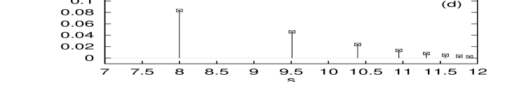
FIG. 5.: Classical averages on rational tori of (a) the identity, (b) $\langle r^{2}\rangle_{p}$, (c) $\langle r\rangle_{p}^{2}$, and (d) the variances ${\rm Var}_{p}r\equiv\langle r^{2}\rangle_{p}-\langle r\rangle_{p}^{2}$ for the circle billiard with radius $R=1$ as functions of the scaled action. Solid lines and crosses: Results of the harmonic inversion of quantum spectra. Dashed lines and squares: Periodic orbit means obtained by classical calculations.

the very good but not absolutely perfect results for the hydrogen atom in a magnetic field in Figs. 3 and 4 may be explained by the different number of quantum states used in the harmonic inversion analysis. For the circle billiard we have calculated more than 30000 states, which is by about a factor of 10 (5.5) times more quantum states than for the hydrogen atom in a magnetic field at scaled energy $\tilde{E}=-0.1$ ($\tilde{E}=-0.5$).

IV Conclusion and outlook

We have extended semiclassical trace formulas for the density of states of regular and chaotic systems, or the density of states weighted with the diagonal matrix elements of smooth operators, to the more general class of non-trace type equations, where the density of states is weighted with the diagonal matrix elements of two operators $\hat{A}$ and $\hat{B}$, i.e., $\rho^{(A,B)}(E)=\sum_{n}\langle n|\hat{A}|n\rangle\langle n|\hat{B}|n\rangle\delta(E-E_{n})$. By the high resolution analysis (harmonic inversion) of the quantum spectra of two different systems, viz. the hydrogen atom in a magnetic field and the circle billiard, we have given numerical evidence that weighting the quantum mechanical density of states with the product of the diagonal matrix elements $\langle n|\hat{A}|n\rangle\langle n|\hat{B}|n\rangle$ is equivalent, on the semiclassical level, to weighting the periodic orbit contributions in the periodic orbit sum with the product of the averages of the corresponding classical observables, $\langle A\rangle_{p}\langle B\rangle_{p}$, where the means are taken along the periodic orbits or resonant tori for chaotic and regular systems, respectively. However, a rigorous mathematical derivation of semiclassical non-trace type formulas appears nontrivial, and would be a challenging task for the further development of semiclassical theories.

There are several useful and important applications of semiclassical non-trace type formulas. For example, it enables the semiclassical approach to matrix element fluctuations. The variances ${\rm Var}_{n}A\equiv\langle n|\hat{A}^{2}|n\rangle-\langle n|\hat{A}|n\rangle^{2}$ of the diagonal matrix elements of a smooth operator $\hat{A}$ are expressed in terms of the variances ${\rm Var}_{p}A\equiv\langle A^{2}\rangle_{p}-\langle A\rangle_{p}^{2}$ of the classical observable $A$ taken along the periodic orbits or resonant tori. Non-trace type formulas also provide the semiclassical approximation to cross-correlated weighted density of states, $\rho_{\alpha\alpha^{\prime}}(E)=\sum_{n}\langle n|\hat{A}_{\alpha}|n\rangle\langle n|\hat{A}_{\alpha^{\prime}}|n\rangle\delta(E-E_{n})$ with a set of smooth operators $\hat{A}_{\alpha}$, $\alpha=1,\dots,D$. The additional classical information obtained from the set of classical observables can be used to significantly improve the convergence properties of semiclassical quantization methods [14].

In this paper we have investigated non-trace type expressions for products of two diagonal matrix elements. These products have been chosen because of the important applications to semiclassical matrix element fluctuations, i.e., the calculation of variances of matrix elements and to the semiclassical quantization method in Ref. [14]. However, our conjecture is not restricted to products of two matrix elements. For example, it appears straightforward to generalize Eqs. 37 and 39 to products of more than two matrix elements and classical periodic orbit means. The most general case of non-trace type equations would be the analysis of functions $f(A_{nn},B_{nn},C_{nn},\dots)$ of one or more diagonal matrix elements, i.e., $\rho^{(f)}(E)=\sum_{n}f(A_{nn},B_{nn},C_{nn},\dots)\delta(E-E_{n})$, which should be obtained semiclassically by multiplying the periodic orbit amplitudes of Gutzwiller’s trace formula or the Berry-Tabor formula with the function $f(\langle A\rangle_{p},\langle B\rangle_{p},\langle C\rangle_{p},\dots)$ of the periodic orbit means of the corresponding classical observables. Certainly the operators and the function $f$ must be smooth. Clearly, further investigations will be necessary to verify that conjecture and to specify the smoothness conditions on operators and functions.

In conclusion, the analysis of non-trace type equations will provide a valuable instrument for extending the relation between quantum mechanical matrix elements on the one side and the periodic orbit means of classical observables on the other.

- [1] M. C. Gutzwiller, J. Math. Phys. 8, 1979 (1967); 12, 343 (1971).
- [2] M. C. Gutzwiller, Chaos in Classical and Quantum Mechanics (Springer, New York, 1990).
- [3] M. V. Berry and M. Tabor, Proc. R. Soc. London A 349, 101 (1976) and J. Phys. A 10, 371 (1977).
- [4] M. V. Berry, Proc. R. Soc. London A 400, 229 (1985).
- [5] D. Wintgen, Phys. Rev. Lett. 58, 1589 (1987).
- [6] P. Cvitanović and B. Eckhardt, Phys. Rev. Lett. 63, 823 (1989).
- [7] M. Sieber and F. Steiner, Phys. Rev. Lett. 67, 1941 (1991).
- [8] M. V. Berry and J. P. Keating, Proc. R. Soc. London A 437, 151 (1992).
- [9] J. Main, V. A. Mandelshtam, and H. S. Taylor, Phys. Rev. Lett. 79, 825 (1997).
- [10] J. Main, V. A. Mandelshtam, G. Wunner, and H. S. Taylor, Nonlinearity 11, 1015 (1998).
- [11] M. Wilkinson, J. Phys. A 21, 1173 (1988).
- [12] B. Eckhardt, S. Fishman, K. Müller, and D. Wintgen, Phys. Rev. A 45, 3531 (1992).
- [13] B. Eckhardt, S. Fishman, J. Keating, O. Agam, J. Main, and K. Müller, Phys. Rev. E 52, 5893 (1995).
- [14] J. Main, K. Weibert, V. A. Mandelshtam, and G. Wunner, Phys. Rev. E (1999), submitted.
- [15] M. Combescure, J. Ralston, and D. Robert, preprint (LPTHE Orsay 97-64).
- [16] O. Bohigas, S. Tomsovic, and D. Ullmo, Phys. Rep. 223, 43 (1993).
- [17] B. Mehlig, Phys. Rev. E 59, 390 (1999).
- [18] H. Friedrich and D. Wintgen, Phys. Rep. 183, 37 (1989).
- [19] H. Hasegawa, M. Robnik, and G. Wunner, Prog. Theor. Phys. Suppl. 98, 198 (1989).
- [20] S. Watanabe, Review of Fundamental Processes and Applications of Atoms and Ions, ed. C. D. Lin, (World Scientific, Singapore, 1993).
- [21] J. Main, V. A. Mandelshtam, and H. S. Taylor, Phys. Rev. Lett. 78, 4351 (1997).
- [22] M. R. Wall and D. Neuhauser, J. Chem. Phys. 102, 8011 (1995).
- [23] V. A. Mandelshtam and H. S. Taylor, Phys. Rev. Lett. 78, 3274 (1997) and J. Chem. Phys. 107, 6756 (1997).
- [24] D. Boosé, J. Main, B. Mehlig, and K. Müller, Europhys. Lett. 32, 295 (1995).
- [25] D. Boosé and J. Main, Phys. Lett. A 217, 253 (1996) and Phys. Rev. E (1999), submitted.