Helicoidal model for DNA opening.

Abstract

We present a new dynamical model of DNA. This model has two degrees of freedom per base-pair: one radial variable related to the opening of the hydrogen bonds and an angular one related to the twisting of each base-pair responsible for the helicoidal structure of the molecule. The small amplitude dynamics of the model is studied analytically : we derive small amplitude envelope solutions made of a breather in the radial variables combined with a kink in the angular variables, showing the role of the topological constraints associated to the helicoidal geometry. We check the stability of the solutions by numerical integration of the motion equations.

I Introduction.

Simple dynamical DNA models have been recently studied [1] to understand the possible basic mechanisms of some biological processes such as denaturation, initiation of the transcription, and transcription. The thermal denaturation has been investigated by Peyrard, Bishop and co-workers [2, 3] with a unidimensional model (PB model) which allows local openings of the hydrogen bonds and formation of denaturation bubbles. The local openings can be analytically described as breather-like objects of small amplitude, which have nevertheless interesting properties: as long as their amplitude is small enough, they can move along the chain, collect energy and grow [4]. They can also be trapped by some local dishomogeneities [5], which suggests that the properties of breathers could allow the formation of the transcription bubble after the interaction with the bound RNA-polymerase.

However, in a realistic description of DNA dynamics, the topological constraints related to the helicoidal structure of the molecule cannot be ignored. Activation or repression effects caused by conformational changes and, in particular, prevention of transcription due to a large positive excess in twist, are known and largely investigated in biology. In fact, during all processes in which the DNA base-pairs open, a local unwinding of the helix follows for topological reasons. Consequently a local extra-twist accumulates at the two ends of the bubble and induces a long range elastic stress. Although the mechanical properties of DNA have recently been the object of a renewed interest[6, 7], previous attempts to take into account the helicoidal structure in the models have been limited to the introduction of the forces that can appear due to the proximity in space of bases which are non-adjacent in the sequence [1].

Our aim here is to build a simple model that takes into account the twist-opening interactions due to the helicoidal molecular geometry. Such a model provides an extension of the PB approach towards a more realistic description of biological processes. It can also be useful for more general studies of the interaction between geometrical conformation and dynamical properties of the molecule referring to the recent mechanical experiments on DNA [8, 9, 10].

In designing such a model each base will be considered as a single, non-deformable object. We introduce two degrees of freedom per base-pair: one radial variable related to the motion of the bases along the diameter that joins their attachment points to the helicoidal backbone, and a twist angle of each base-pair defined by the angle between this diameter and a reference direction. This twist angle, which increases from one base-pair to the next one, is responsible for the helicoidal structure of the molecule. From the resulting Lagrangian the equation of motion for small displacements with respect to the equilibrium position are written. We then derive analytical approximated solutions for the small amplitude nonlinear distortions of the molecule. As suggested by the helicoidal geometry we show that the radial breather-like opening is associated to an angular un-twisting of the molecule. We finally present the results of numerical simulations of the dynamics showing that these solutions are stable for long periods of time and can move along the chain.

The analytical method of derivation of the envelope soliton solution of the equation of motion used in this work has been proposed and developed extensively in a previous paper [15]. The reader is referred to this work to better follow the technical steps of our calculation.

II The helicoidal model.

In the PB model [2], the bases are point masses allowed to move only in the direction of the hydrogen bonds that connect them. A Morse potential describes the effect of these bonds, while neighboring bases along the same strand are harmonically coupled, simulating the stacking interactions.

Similarly, in our model the group made of a sugar ring and its connected base is treated simply as a point mass (without distinction between the different base types); the phosphate backbone between two base-pairs is modelised as an elastic rod. The additional twist motion is now introduced by allowing the two bases in each pair to move in the base-pair plane instead of constraining them on a line. It is convenient to choose a polar coordinate system (Fig. 1). The model does not attempt to describe the acoustic motions of the molecule since only the stretching of the base-pair distance is considered. This amounts to fixing the center of mass of the base pair, i.e. the two bases in a pair are constrained to move symmetrically with respect to the axis of the molecule. Then, to describe the stretching of a base pair and the variation of the helicoidal twist we need only two degrees of freedom per base pair: the coordinates ${r}_{n}$ and ${\varphi}_{n}$ of one of the two bases with respect to a fixed reference frame.

As in the PB model, a Morse potential describes the hydrogen bonds linking bases in a pair with an equilibrium distance $R_{0}$.

A proper choice of the coupling between radial and angular variables has to reproduce the equilibrium helicoidal structure. In DNA, the latter originates from the competition between the hydrophobic effect (that tends to eliminate water from the core of the molecule by bringing the neighboring base-pair planes closer) the electrostatic repulsion between neighboring base planes (which has the opposite effect) and the rigidity of the two strands (that separates the external ends of the base pairs by essentially a fixed length related to the phosphate length) [12]. We combine the first two forces in a unique stacking effect that fixes base-plane distance $h$ in the model. As the equilibrium backbone length $L$ is greater than $h$, it is then necessary to incline the strands in the typical helicoidal structure to minimize the energy.

The geometrical parameters $h$ and $R_{0}$ have been chosen to match the structure of B-DNA. Then, in order to impose an equilibrium twist angle ${\varphi}_{n}-{\varphi}_{n-1}=\pm{\Theta}_{0}$ between two consecutive base pairs, we select the equilibrium length $L$ of the springs representing the phosphate backbone to be

$$L=\sqrt{{h}^{2}+4{R}_{0}^{2}\sin^{2}\big{(}{{\Theta}_{0}\over 2}\big{)}}\,>\,h$$ (1)

However, because of the invariance of $L$ with respect to the sign of ${\Theta}_{0}$, the elastic rods rigidity is not sufficient to guarantee the correct helicoidal shape. A zig-zag structure with a random succession of $\pm{\Theta}_{0}$ would as well minimize the energy of the system. This can be avoided by adding a three-body curvature term to the Lagrangian, that imposes a continuity between the differences ${\varphi}_{n}-{\varphi}_{n-1}$ and ${\varphi}_{n+1}-{\varphi}_{n}$.

The final Lagrangian is written considering the expression of the three-dimensional distance between the two bases along the strand (Fig. 1); it reads

$${\cal L} = \sum_{n}\big{(}m{\dot{{r}_{n}}}^{2}+m{{r}_{n}}^{2}{\dot{{\varphi}_{n}}}^{2}\big{)}-D\big{(}e^{-\alpha({r}_{n}-{R}_{0})}-1\big{)}^{2}$$ (2)

$$- \sum_{n}K{\big{(}\sqrt{{h}^{2}+{r}_{n-1}^{2}+{r}_{n}^{2}-2{r}_{n-1}{r}_{n}\cos({\varphi}_{n}-{\varphi}_{n-1})}-L\big{)}}^{2}$$ (3)

$$- \sum_{n}G_{0}\,{\big{(}{\varphi}_{n+1}+{\varphi}_{n-1}-2{\varphi}_{n}\big{)}}^{2}\;$$ (4)

where $m$ is the base mass, $D$ and $\alpha$ are the depth and width of the Morse potential well (without distinction between double and triple hydrogen bonds), $K$ is the backbone elastic constant and $G_{0}$ the backbone curvature constant.

The results presented below have been obtained with, $m=300u.m.a.$, $D=0.04eV$, $\alpha=4.45$ Å^-1 that are the same valued adopted in the PB model, and with $K=1.0eV$ Å^-2 and $G_{0}=KR_{0}^{2}/2$. We intend to refine these values in future statistical mechanics studies by comparing the predictions of the present model with some available experimental data, eg. the temperature of DNA denaturation and the rigidity of the molecule [13].

For the geometrical parameters we adopt the B-DNA values $R_{0}\approx 10.0$ Å, ${\Theta}_{0}=36^{\circ}$ and $h=3.4$ Å.

One can simplify the Lagrangian by introducing the adimensional variables $r^{\prime}_{n}=\alpha r_{n}$, the rescaled time $t^{\prime}=\sqrt{D\alpha^{2}/m}\,t$ and the renormalized parameters

$$K^{\prime} = K/D\alpha^{2}$$ (5)

$${\cal G^{\prime}} = G_{0}/D$$ (6)

$$R^{\prime}_{0} = \alpha R_{0}$$ (7)

$$h^{\prime} = \alpha h$$ (8)

$$L^{\prime} = \alpha L\,.$$ (9)

In the following the new variables will be written without primes.

We perform an expansion of the energy of the backbone springs in (2) up to the second order around the equilibrium position:

$$y_{n} = r_{n}-R_{0}\,$$ (10)

$${\phi}_{n} = R_{0}(\,{\varphi}_{n}-n{\Theta}_{0}\,)\,,$$ (11)

obtaining

$${\big{(}\sqrt{{h}^{2}+{r}_{n-1}^{2}+{r}_{n}^{2}-2{r}_{n-1}{r}_{n}\cos({\varphi}_{n}-{\varphi}_{n-1})}-L\big{)}^{2}}\simeq$$ (12)

$${{R_{0}^{2}}\over{L^{2}}}{\big{[}\sin{{\Theta}_{0}}({\phi}_{n}-{\phi}_{n-1})+(y_{n}+y_{n-1})(1-\cos{\Theta_{0}})\big{]}}^{2}\,.$$ (13)

We also expand the Morse potential up to the fourth order in $y_{n}$

$$\big{(}e^{-{y}_{n}}-1\big{)}^{2}=\frac{1}{2}y_{n}^{2}-\frac{1}{2}y_{n}^{3}+\frac{7}{24}y_{n}^{4}+O({y_{n}}^{5})\,.$$ (14)

The difference in the order of the two expansions is consistent with our parameter choice.

With these expansions, the equations of motion become:

$${\ddot{y}}_{n} = \big{(}1+{{y_{n}}\over{R_{0}}}\big{)}{{1}\over{R_{0}}}{\dot{\phi}}_{n}^{2}-(y_{n}-{{3}\over{2}}y_{n}^{2}+{{7}\over{6}}y_{n}^{3})-K_{yy}({y}_{n+1}+{y}_{n-1}+2{y}_{n})$$ (16)

$$-{{K_{y\phi}}\over{2}}({\phi}_{n+1}-{\phi}_{n-1})$$

$${\ddot{\phi}}_{n} = K_{\phi\phi}({\phi}_{n+1}+{\phi}_{n-1}-2{\phi}_{n})$$ (17)

$$- G({\phi}_{n+2}+{\phi}_{n-2}-4{\phi}_{n+1}-4{\phi}_{n-1}+6{\phi}_{n})$$ (19)

$$+{{K_{y\phi}}\over{2}}({y}_{n+1}-{y}_{n-1})-\frac{2}{R_{0}}{\dot{y}}_{n}{\dot{\phi}}_{n}-\frac{2}{R_{0}}{{y}}_{n}{\ddot{\phi}}_{n}-\frac{2}{R_{0}^{2}}y_{n}{\dot{y}}_{n}{\dot{\phi}}_{n}-\frac{1}{R_{0}^{2}}y_{n}^{2}{\ddot{\phi}}_{n}$$

where

$$K_{yy} = \big{(}KR_{0}^{2}/L^{2}\big{)}{(1-\cos{\Theta}_{0})}^{2}\;,$$ (20)

$$K_{\phi\phi} = \big{(}KR_{0}^{2}/L^{2}\big{)}{(\sin^{2}{\Theta}_{0})}\;,$$ (21)

$$K_{y\phi} = 2\big{(}KR_{0}^{2}/L^{2}\big{)}(\sin{\Theta}_{0})(1-\cos{\Theta}_{0})\;$$ (22)

$$G = {\cal G}/R_{0}^{2}\,.$$ (23)

The constants $K_{yy},K_{\phi\phi}$ are the effective elastic constants respectively for the base pairs opening and the twist rotation, $K_{y\phi}$ is the coupling constant between stretching and twist; these three constant are geometrically related.

III Localized breather-like solutions.

We now look for nonlinear localized solutions, characterized by the propagation of a coherent collective structure on a time scale greater than the time scale of the vibrations of each particle around its equilibrium position.

According to the method developped in [15] we first solve for a wave packet solution of the linearized system with weak dispersion. This amounts to solving

$$(\hat{J}(q)-\omega^{2}_{l}(q))\vec{V}_{l}(q)=0$$ (24)

where $l=+,-$ is the branch index and

$$\hat{J}(q)=\left(\matrix{1+2K_{yy}(1+\cos{q})&iK_{y\phi}\sin{q}\cr-iK_{y\phi}\sin{q}&2K_{\phi\phi}(1-cos{q})+G(6-8\cos{q}+2\cos{2q})}\right)\equiv\left(\matrix{a&c\cr c^{*}&b}\right)$$ (25)

finding the eigenvalues and eigenvectors

$$\omega^{2}_{\pm}(q)=\frac{1}{2}(a+b\pm\sqrt{(a-b)^{2}+4|c|^{2}}\;)$$ (26)

$$\vec{V}^{\pm}(q)={\cal N_{\pm}}\left(\begin{array}[]{c}1\\ \frac{a-\omega_{\pm}^{2}}{-c}\end{array}\right)$$ (27)

where ${\cal N_{\pm}}$ are the vector norms.

Then we apply a perturbative expansion of the system (24) around one normal mode. We have chosen as carrier wave a mode ($q_{0},\omega_{+}=\omega_{+}(q_{0})$) on the optical branch and with a small wave number that corresponds to a prevalently radial excitation weakly oscillating. In fact, keeping in mind DNA opening, we shall calculate the behaviour of a localized bubble-like radial distorsion and the induced angular dynamics. We obtain the wave-packet group velocity from the first order eigenvalue correction

$$\omega_{+}^{(1)}=\frac{{\vec{V}^{+*}}\hat{J^{\prime}}\vec{V}^{+}}{2\omega_{+}}=\frac{1}{2\omega_{+}}(a^{\prime}|{V}^{+}_{1}|^{2}+c^{\prime}{V}^{+*}_{1}{V}^{+}_{2}+c^{\prime*}{V}^{+*}_{2}{V}^{+}_{1}+b^{\prime}|{V}^{+}_{2}|^{2})\quad,$$ (28)

where the primes indicate the derivatives with respect to $q$ calculated at $q_{0}$. We then obtain the correction to the eigenvector $\vec{V}^{+}$

$$\vec{V}^{(1)}=\alpha\vec{V}^{-}$$ (29)

$$\alpha=\frac{{\vec{V}^{-*}}\hat{J}^{\prime}\vec{V}^{+}}{\omega_{+}^{2}-\omega_{-}^{2}}=\frac{a^{\prime}{V}^{-*}_{1}{V}^{+}_{1}+c^{\prime}{V}^{-*}_{1}{V}^{+}_{2}+c^{\prime*}{V}^{-*}_{2}{V}^{+}_{1}+b^{\prime}{V}^{-*}_{2}{V}^{+}_{2}}{\omega_{+}^{2}-\omega_{-}^{2}}$$ (30)

and from the second order eigenvalue correction the group velocity dispersion is obtained as

$$\omega_{+}^{(2)} = \frac{1}{\omega_{+}}({\vec{V}}^{+*}\frac{\hat{J}^{\prime\prime}}{2}\vec{V}^{+}-{\omega_{+}^{(1)}}^{2}+\frac{|{\vec{V}^{-*}}\hat{J}^{\prime}\vec{V}^{+}|^{2}}{\omega^{2}_{+}-\omega^{2}_{-}})\$$ (31)

$$= \frac{1}{\omega_{+}}(\frac{1}{2}(a^{\prime\prime}|{V}^{+}_{1}|^{2}+c^{\prime\prime}{V}^{+*}_{1}{V}^{+}_{2}+c^{\prime\prime*}{V}^{+*}_{2}{V}^{+}_{1}+b^{\prime\prime}|{V}^{+}_{2}|^{2})-{\omega_{+}^{(1)}}^{2}+|\alpha|^{2}(\omega_{+}^{2}-\omega_{-}^{2}))$$ (32)

We now take into account the nonlinearity. We look for a small amplitude solution. The expansion parameter $\epsilon$ for the solution is introduced to solve the equation of motion at increasing order of accuracy inserting the nonlinear terms in a progressive way. This iterative expansion is combined with the expansion in multiple scales for the weak dispersive wave packet. The latter requires the introduction of the variables $x_{1}=\epsilon x,t_{1}=\epsilon t,t_{2}=\epsilon^{2}t$ for the slowly varying amplitudes, where $\epsilon$ is the same parameter as before. We look then for a solution of the form

$$\vec{E}(n) = \epsilon e^{i(q_{0}n_{0}-\omega_{+}t_{0})}(\vec{V}^{+}-i\epsilon\vec{V}^{(1)}\frac{\partial}{\partial x_{1}})A(x_{1},t_{1},t_{2})+\epsilon\vec{\sigma}(x_{1},t_{1},t_{2})$$ (33)

$$+ \epsilon^{2}e^{2i(q_{0}n_{0}-\omega_{+}t_{0})}\vec{\gamma}(x_{1},t_{1},t_{2})+\epsilon^{2}\vec{\mu}(x_{1},t_{1},t_{2})\,$$ (34)

where the first term is the wave packet, the second term arise because the linear system admits a constant solution with a non zero second component, corresponding to the null column of $\hat{J}(0)$. The constant and second harmonic $\epsilon^{2}$ terms are induced by the quadratic nonlinearity in the equation of motion.

We have now to determine the slowly variyng amplitudes $A(x_{1},t_{1},t_{2}),\vec{\sigma}(x_{1},t_{1},t_{2}),\vec{\gamma}(x_{1},t_{1},t_{2}),\vec{\mu}(x_{1},t_{1},t_{2})$

From the $O(\epsilon^{2})$ equation of motion we obtain for the second harmonic terms the system of equations:

$$(\hat{J}(2q_{0})-4\omega_{+}^{2})\vec{\gamma}=\left(\matrix{3/2{V_{1}^{+}}^{2}-\frac{\omega_{+}^{2}}{R_{0}}{V_{2}^{+}}^{2}\cr\frac{4\omega_{+}^{2}}{R_{0}}V_{1}^{+}V_{2}^{+}}\right)\;A^{2}\;.$$ (35)

Its solution may be written as $\vec{\gamma}=\vec{\gamma_{c}}A^{2}$ and for the constant terms

$$\hat{J}(0)\vec{\mu}-i\hat{J^{\prime}}(0)\frac{\partial}{\partial x_{1}}\vec{\sigma}=\left(\matrix{3|{V_{1}^{+}}|^{2}+\frac{2\omega_{+}^{2}}{R_{0}}|{V_{2}^{+}}|^{2}\cr 0}\right)\;|A|^{2}\quad.$$ (36)

Inserting the value of $\hat{J}(0)$ from (25) in the above matricial equation, we obtain the identity

$$(1+4K_{yy})\mu_{1}+K_{y\phi}\frac{\partial}{\partial x_{1}}\sigma_{2}=(3|{V_{1}^{+}}|^{2}+\frac{2\omega_{+}^{2}}{R_{0}}|{V_{2}^{+}}|^{2})\;|A|^{2}$$ (37)

that does not allow to determine the two unknown variables. We have thus to consider the $O(\epsilon^{3})$ system of equations for the constant terms

$$-i\hat{J^{\prime}}(0)\frac{\partial}{\partial x_{1}}\vec{\mu}-\hat{J^{\prime\prime}}(0)\frac{\partial^{2}}{\partial x_{1}^{2}}\vec{\sigma}=\left(\matrix{\frac{2i\omega_{+}}{R_{0}}|{V_{2}^{+}}|^{2}(A^{*}\frac{\partial A}{\partial t_{1}}-\frac{\partial A^{*}}{\partial t_{1}}A)\cr\frac{-2i\omega_{+}}{R_{0}}({V_{2}^{+}}^{*}V_{1}^{+}-{V_{1}^{+}}^{*}V_{2}^{+})\frac{\partial}{\partial t_{1}}|A|^{2}}\right)$$ (38)

corresponding to the two equations:

$$K_{y\phi}\frac{\partial}{\partial x_{1}}\mu_{2} = \frac{2i\omega_{+}}{R_{0}}|{V_{2}^{+}}|^{2}(A^{*}\frac{\partial A}{\partial t_{1}}-\frac{\partial A^{*}}{\partial t_{1}}A)$$ (39)

$$-K_{y\phi}\frac{\partial}{\partial x_{1}}\mu_{1}-2K_{\phi\phi}\frac{\partial^{2}}{\partial x_{1}^{2}}\sigma_{2} = \frac{-2i\omega_{+}}{R_{0}}({V_{2}^{+}}^{*}V_{1}^{+}-{V_{1}^{+}}^{*}V_{2}^{+})\frac{\partial}{\partial t_{1}}|A|^{2}$$ (40)

The equation (39) gives $\mu_{2}$ as a function of $A$. The equation (40) can be integrated using the wave packet property $\frac{\partial A}{\partial t_{1}}=-\omega_{+}^{(1)}\frac{\partial A}{\partial x_{1}}$. We then obtain from (37), (40) the following system for $\mu_{1}$ and $\sigma_{2}$,

$$\left(\matrix{1+4K_{yy}&K_{y\phi}\cr-K_{y\phi}&-2K_{\phi\phi}}\right)\;\left(\matrix{\mu_{1}\cr\frac{\partial\sigma_{1}}{\partial x_{1}}}\right)=\left(\matrix{3|{V_{1}^{+}}|^{2}+\frac{2\omega_{+}^{2}}{R_{0}}|{V_{2}^{+}}|^{2}\cr\frac{2i\omega_{+}\omega_{+}^{(1)}}{R_{0}}({V_{2}^{+}}^{*}V_{1}^{+}-{V_{1}^{+}}^{*}V_{2}^{+})}\right)\;|A|^{2}\quad,$$ (41)

the solutions of which may be written as

$$\mu_{1}={\mu_{1}}_{c}|A|^{2}$$ (42)

$$\sigma_{2}=\sigma_{c}\int|A|^{2}dx_{1}$$ (43)

The nonlinear $O(\epsilon^{3})$ terms in $\exp{i(q_{0}n_{0}-\omega_{+}t_{0})}$ in the equation of motion give rise to the nonlinearity that balances the group velocity dispersion of the wave packet. We indeed obtain the following Non Linear Schrödinger (NLS) equation for the envelope $A$ expressed in a frame moving at velocity $\omega_{+}^{(1)}$ (variables $S=x_{1}-\omega_{+}^{(1)}t_{1},\tau=t_{2}$):

$$iA_{\tau}+PA_{SS}+Q{|A|}^{2}A=0$$ (44)

with

$$P = \frac{\omega_{+}^{(2)}}{2}\;,$$ (45)

$$Q = {{{(Q_{1}{V_{1}^{+}}^{*}+Q_{2}{V_{2}^{+}}^{*})}}\over{2\omega_{+}}}\;,$$ (46)

where

$$Q_{1} = -\frac{7}{2}|V_{1}^{+}|^{2}V_{1}^{+}+\frac{\omega_{+}^{2}}{R_{0}^{2}}(2V_{1}^{+}|V_{2}^{+}|^{2}-{V_{1}^{+}}^{*}{V_{2}^{+}}^{2})+$$ (48)

$$3{V_{1}^{+}}^{*}{\gamma_{1}}_{c}+\frac{4\omega_{+}^{2}}{R_{0}}{V_{2}^{+}}^{*}{\gamma_{2}}_{c}+3V_{1}^{+}{\mu_{1}}_{c}$$

$$Q_{2} = \frac{\omega_{+}^{2}}{R_{0}}(4{V_{1}^{+}}^{*}{\gamma_{2}}_{c}-2{V_{2}^{+}}^{*}{\gamma_{1}}_{c})+\frac{2\omega_{+}^{2}}{R_{0}}V_{2}^{+}{\mu_{1}}_{c}-$$ (50)

$$\frac{2\omega_{+}^{2}}{R_{0}^{2}}{V_{1}^{+}}^{2}{V_{2}^{+}}^{*}+\frac{\omega_{+}^{2}}{R_{0}^{2}}(2|V_{1}^{+}|^{2}V_{2}^{+}+{V_{1}^{+}}^{2}{V_{2}^{+}}^{*})\quad.$$

If $PQ>0$, equation (44) has an envelope soliton solution

$$A(S,\tau)={\cal A}\ \mbox{sech}{[{{1}\over{L_{e}}}(S-u_{e}\tau)]}\exp{[i{{u_{e}}\over{2P}}(S-u_{c}\tau)]}$$ (51)

where

$${\cal A}=\sqrt{{{u_{e}^{2}-2u_{e}u_{c}}\over{2PQ}}}$$ (52)

$$L_{e}={{2P}\over{\sqrt{u_{e}^{2}-2u_{e}u_{c}}}}$$ (53)

are respectively the amplitude and the width of the curve.

Once the NLS equation is solved for $A(S,\tau)$, we have $\sigma_{2}$, $\vec{\gamma}$, $\vec{\mu}$ (solving (39) we obtain $\mu_{2}={\mu_{2}}_{c}\int|A|^{2}dx_{1}$) and then the complete solution

$$y = \epsilon(V_{1}^{+}-i\epsilon V_{1}^{(1)}\frac{\partial}{\partial x_{1}})Ae^{i\theta}+c.c.+\epsilon^{2}{\gamma_{1}}_{c}A^{2}e^{2i\theta}+c.c.+\epsilon^{2}{\mu_{1}}_{c}{|A|}^{2}+O(\epsilon^{3})$$ (54)

$$\phi = \epsilon\sigma_{c}\int{|A|}^{2}dx_{1}+\epsilon(V_{2}^{+}-i\epsilon V_{2}^{(1)}\frac{\partial}{\partial x_{1}})Ae^{i\theta}+c.c.+\epsilon^{2}{\gamma_{2}}_{c}A^{2}e^{2i\theta}+c.c.+\epsilon^{2}{\mu_{2}}_{c}\int{|A|}^{2}dx_{1}+O(\epsilon^{3})\,.$$ (55)

where $\theta=(q_{0}n_{0}-\omega_{+}t_{0})\,.$ The final result can be rewritten in the following form:

$$y = 2\epsilon{V_{1}}^{+}{\cal A}\mbox{sech}{[\eta(x-V_{e}t)]}\cos{({\cal K}x-{\Omega}t)}$$ (56)

$$+ \epsilon^{2}{V_{1}}^{(1)}{\cal A}\mbox{sech}{[\eta(x-V_{e}t)]}\left[\frac{-2}{L_{e}}\tanh{(\eta(x-V_{e}t))}\sin{({\cal K}x-{\Omega}t)}+{{u_{e}}\over{P}}\cos{({\cal K}x-{\Omega}t)}\right]$$ (57)

$$+ 2\epsilon^{2}{\gamma_{1}}_{c}{\cal A}^{2}{\mbox{sech}}^{2}{[\eta(x-V_{e}t)]}\cos{(2{\cal K}x-2{\Omega}t)}$$ (58)

$$+ {\mu_{1}}_{c}\epsilon^{2}{\cal A}^{2}{\mbox{sech}}^{2}{[\eta(x-V_{e}t)]}+O(\epsilon^{3})$$ (59)

$$\phi = \epsilon(\sigma_{c}+\epsilon{\mu_{2}}_{c})L_{e}{\cal A}^{2}\tanh{(\eta(x-V_{e}t))}-2\epsilon{\cal A}|V_{2}^{+}|\mbox{sech}{[\eta(x-V_{e}t)]}\sin{({\cal K}x-{\Omega}t)}$$ (60)

$$- \epsilon^{2}{V_{2}}^{(1)}{\cal A}\mbox{sech}{[\eta(x-V_{e}t)]}\left[\frac{2}{L_{e}}\tanh{(\eta(x-V_{e}t))}\cos{({\cal K}x-{\Omega}t)}+{{u_{e}}\over{P}}\sin{({\cal K}x-{\Omega}t)}\right]$$ (61)

$$- 2\epsilon^{2}|{\gamma_{2}}_{c}|{\cal A}^{2}{\mbox{sech}}^{2}{[\eta(x-V_{e}t)]}\big{[}\sin{(2{\cal K}x-2{\Omega}t)}\big{]}+O(\epsilon^{3})$$ (62)

where

$$\eta = {{\epsilon}\over{L_{e}}}$$ (63)

$$V_{e} = {\omega_{+}}^{(1)}+\epsilon u_{e}$$ (64)

$$V_{c} = {\omega_{+}}^{(1)}+\epsilon u_{c}$$ (65)

$${\cal K} = q_{0}+{{\epsilon u_{e}}\over{2P}}$$ (66)

$${\Omega} = \omega_{+}+{{\epsilon u_{e}}\over{2P}}V_{c}\,.$$ (67)

Fig. 3 shows the analytical solution (56),(60) in the original variables (not renormalized), as a function of $x$ and $t$. Fig. 4 displays the results of numerical simulations of the system described by the complete Lagrangian (1) starting from the analytical solution (56),(60) for $t=0$ as an initial condition. We have chosen the carrier wavevector $q_{0}=0.1$.

The shape of the solution is best seen on Fig. 3a, 3b which show for a few periods the radial displacement $r_{n}(t)-R_{0}$ (Fig. 3a) and of the angular displacement $\varphi_{n}(t)$ (Fig. 3b), while Fig. 3c represents the twist angle, i.e. the difference between neighboring angles, $\Delta\varphi_{n}(t)$. As in the PB model the radial motion has the shape of an asymmetric breather, the stretching of the base-pair distance being larger than its compression, as expected from the asymmetry of the Morse potential. The corresponding angular motion clearly exhibits a kink structure due to the non oscillating term $\sigma(x,t)$; a small oscillating part due to the other terms in (60) is superimposed on it.

The shape of the solution agrees with the geometrical properties of the molecule related to its helicoidal structure. It shows, as expected, that our model can indeed describe the local untwisting which should be coupled with the radial breather due to the geometrical constraints. To make this clearer we plot in Fig. 3c the evolution of the twist angle. In addition to the local opening, small periodic overtwists on the boundaries, coming from the oscillating part of the solutions are visible. The coupled breather and kink solutions move with a peak velocity $V_{e}=\omega_{+}^{(1)}+\epsilon u_{e}$ without changing their internal structure.

The long time evolution of the initial condition, calculated with the full Lagrangian and shown in Fig. 4, attests that the local excitation is very stable. It does not radiates energy with the exception of a small initial transient that could be eliminated with absorbing boundary conditions. During all the simulation time the total energy lost with the absorbing conditions is less than $10^{-5}$ of the total energy. It should be noticed that Fig. 4 does not show the actual oscillations due to the large sampling time used to produce the graph. The slow oscillation visible on Fig. 4 is due to a beating between the actual oscillation and the sampling time. Fig. 4 shows in fact about 2230 oscillations which proves the exceptional stability of the breather in the helicoidal structure and the ability of the geometrical nonlinearity and of the nonlinearity coming from the Morse potential to keep the energy localized.

As our solution has been obtained with a small amplitude expansion, we should not expect it to be a good solution when its amplitude increases to much. This can be seen on the results of a numerical simulation starting from a much larger amplitude (Fig. 5). In this case the initial condition decays very fast and radiates energy before stabilizing to a breather which has still a pretty high amplitude and which is localized on about 6 sites (width at half height). Although it is very narrow the breather is still mobile in the system and it is accompanied by a sharp kink as expected from the geometrical constraints. The solution reached after the transient is stable as shown in Fig. 5c: although the simulation has been run with absorbing boundary conditions, the energy tends to stabilize once the radiated waves have been dissipated at the ends of the molecule. In all the solutions described above the breather frequency $\Omega$ remains in the gap between the two branches so that the breather does not emit acoustic phonons.

IV Conclusion

In conclusion we have proposed a two-variable helicoidal DNA model that, from a biological point of view, can be a better starting point than the PB model for the studies of all the DNA dynamical processes involving internal openings. Our model also describes the untwisting that accompanies the base-pair stretching because of the helicoidal molecular geometry. We analytically derive, using the method introduced in [15], a breather like solution in the radial variable coupled with an angular solution dominated by a non oscillating kink-like term. A further step will be the study of the formation of this kind of excitation in presence of a thermal bath and of the onset of thermal denaturation. This will be useful in determining the model parameters by comparison with denaturation temperature experimental data. Furthermore we expect to find interesting thermodynamic properties due to long range effect generated by the helicoidal DNA structure.

As far as biological processes are concerned, the model may however still lack some relevant features, in particular the possibility of bending and stretching of the molecule. In order to obtain a stretchable molecule axis we can simply replace the rigid constraint of fixed base planes distance $h$ with an elastic term which leads to the introduction of a third degree of freedom with a new elastic constant. This could be a link to some recent experimental studies of the mechanical response of a DNA molecule to some twisting and stretching forces [8, 9, 10]. Anyway the model contains in its possible dynamical behaviors some other important features, as e.g. the possibility of local transitions from right hand B-DNA to left hand Z-DNA, related to the curvature term in the Lagrangian depending on the constant $G_{0}$. Our model is, finally, a first attempt to insert in simple DNA dynamical model topological constraints that are of great interest in today’s biological studies.

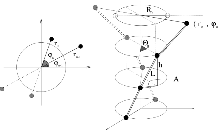
FIG. 1.: Fig. 1: Choice of variables (left) and the schematic view (right) of the model. The n-th base-pair is represented with its radial and angular displacements $(r_{n},\varphi_{n})$ with respect to a fixed external reference frame. Neighbouring base-pairs are linked along the two strands by elastic rods with equilibrium length $L$. $R_{0}$, $\Theta_{0}$ and $h$ are the geometrical parameters of the model, with values deduced from the real B-DNA geometry.

FIG. 2.: Fig. 2: Dispersion curves for the linearized model with $K^{\prime}=K/D\alpha^{2}=1.26$, ${\cal G^{\prime}}=G_{0}/D=K^{\prime}/2\,{R^{\prime}}_{0}^{2}$.

FIG. 3.: Fig. 3a: Analytical solution (56), (60): we show here the radial displacement $r_{n}(t)-R_{0}$, obtained with the model parameters indicated below and with solution parameters $\epsilon=0.1$, $ue=-0.1$, $uc=0.1$. The typical breather oscillation is clearly visible; its period is of $105.1$ time units ($1t.u.=1.0210^{-14}s$). The amplitude $2\epsilon{\cal A}/\alpha$ and the half heigth width, which is about $2.77L_{e}/\epsilon$, are respectively $0.016$ Åand $20\,b.p$.

FIG. 4.: Fig. 3b: Analytical solution (56), (60): the corresponding angular displacement $\varphi_{n}(t)$. The main contribution to this solution is the kink-like term $\epsilon\sigma_{c}L_{e}{\cal A}^{2}\tanh{(\eta(x-V_{e}t))}$ of (60).

FIG. 5.: Fig. 3c: Analytical solution (56), (60): the twist angle, given by the difference between neighboring angles, $\Delta\varphi_{n}(t)$. We stress that the breather opening mode in the radial variables corresponds to an untwisted region.

FIG. 6.: Fig. 4a: Numerical integration (obtained with a Runge Kutta algorithm) of the initial condition which corresponds to the analytical solution of Fig. 3. The amplitude and width parameters preserve their initial values $2\epsilon{\cal A}\sim 0.016$ Åand $2.77L_{e}/\epsilon\sim 20\,b.p.$ with good accuracy, as well as the oscillation period. The total simulation time corresponds to $2234$ oscillation periods. We introduce here absorbing boundary conditions to avoid noise effects produced by reflection of the small amount of radiated energy (less then $10^{-5}$ of the total energy).

FIG. 7.: Fig. 4b: Angular displacement $\varphi_{n}(t)$ generated by the numerical integration of the same initial conditions.

FIG. 8.: Fig. 4c: Numerical integration of the same initial conditions, twist angle.

FIG. 9.: Fig. 5a: Numerical integration of an initial condition obtained with solution parameters $\epsilon=0.2$, $ue=-0.2$, $uc=0.6$. We perform again the simulation with absorbing boundary conditions. The initial amplitude is $2\epsilon{\cal A}=0.1$ Åand the half height width $2.77L_{e}/\epsilon\sim 4\,b.p.$ This initial solution is not stable. The initial radiation is clearly visible. However, after some time, the system tends to stabilize to a smaller breather+kink mode with amplitude $2\epsilon{\cal A}\sim 0.07$ and width $2.77L_{e}/\epsilon\sim 6\,b.p.$ (We stress that the apparent slow modulation of the maximum amplitudes and the apparent oscillation period are due to the beating between the effective oscillation and the sampling time.)

FIG. 10.: Fig. 5b: Numerical integration for the same parameters as in Fig. 5a, angular displacement $\varphi_{n}(t)$.

FIG. 11.: Fig. 5c: Total system energy during the simulation with parameters as in Fig. 5a. The loss of energy is due to the absorbtion at the boundaries and represent essentially the radiative part. After the initial transition to the smaller amplitude breather+kink mode the energy tends to stabilize.

REFERENCES

• [1] G.Gaeta, C. Reiss, M. Peyrard, T. Dauxois Simple Models of Non-Linear DNA Dynamics, Rivista del Nuovo Cimento 17, 1 (1994) and references herein;
• [2] M. Peyrard, A.R. Bishop Statistical Mechanics of a Nonlinear Model for DNA Denaturation, Phys. Rev. Letters 62, 2755 (1989);
• [3] T. Dauxois, M. Peyrard, Entropy-driven transition in a one-dimensional system, Phys. Rev. E 51, 4027 (1995);
• [4] O.Bang, M. Peyrard, Generation of High-energy Localized Vibrational Modes in Nonlinear Klein-Gordon Lattices, Phys. Rev. E 53, 4143 (1996);
• [5] J.L, Ting, M. Peyrard, Effective breather trapping mechanism for DNA transcription, Phys. Rev. E 53, 1011 (1996);
• [6] J.F. Marko and E.D. Siggia, Bending and twisting elasticity of DNA. Macromolecules 27, 981-988 (1994)
• [7] J.F. Marko and E.D. Siggia, Fluctuations and supercoiling of DNA. Science 265, 506-508 (1994)
• [8] S. Smith, Y. Cui, C. Bustamante Overstretching B-DNA: The Elastic Response of Individual Double-Stranded and Single Stranded DNA Molecules, Science 271, 795 (1996);
• [9] T. R. Strick, J. F. Allemand, D. Bensimon, A. Bensimon, V. Croquette The Elasticity of a Single Supercoiled DNA Molecule Science 271,1835 (1996);
• [10] U. Bockelmann, B. Essevaz-Roulet, F, Heslot Molecular Stick-Slip Motion Revealed by Opening DNA with Piconewton Forces, Phys. Rev. Letters 79, 4489 (1997);
• [11] M. Remoissenet, Low Amplitude Breather and Envelope Solitons in Quasi-one-dimensional Physical Models, Phisical Review B, 33, 2386 (1996);
• [12] C. R. Calladine, H. Drew Understanding DNA, (Academic Press, London, 1992);
• [13] C. Bouchiat, M. Mezard Elasticity of a Supercoiled DNA Molecule, Phys. Rev. Letters 80, 1556 (1998);
• [14] T. Dauxois, M. Peyrard, C.R. Willis Discreteness effects on the formation and propagation of breathers in nonlinear Klein-Gordon equations, Phys. Rev. E 48, 4768 (1993);
• [15] S. Cocco, M. Barbi, M. Peyrard, submitted to Phys. Lett. A.
Refer to caption