Spectrum of stochastic evolution operators: local matrix representation approach

Abstract

A matrix representation of the evolution operator  associated with a nonlinear stochastic flow with additive noise is used to compute its spectrum. In the weak noise limit a perturbative expansion for the spectrum is formulated in terms of local matrix representations of the evolution operator centered on classical periodic orbits. The evaluation of perturbative corrections is easier to implement in this framework than in the standard Feynman diagram perturbation theory. The result are perturbative corrections to a stochastic analog of the Gutzwiller semiclassical spectral determinant computed to several orders beyond what has so far been attainable in stochastic and quantum-mechanical applications.

I Introduction

Any dynamical evolution that occurs in nature is affected by noise. In a neuronal system the noise might be comparable in magnitude to purported underlying deterministic dynamics; in celestial mechanics the degrees of freedom omitted from a particular set of equations may be accounted for by very weak noise. Our task here and in two preceding papers [1, 2] is to systematically account for the effects of noise on measurable properties such as dynamical averages[3] in classical chaotic dynamical systems.

The theory is also closely related to the semiclassical expansions based on Gutzwiller’s formula for the trace in terms of classical periodic orbits [4] in that both are perturbative theories (in the noise strength or $\hbar$) derived from saddlepoint expansions of a path integral containing a Cantor set of unstable stationary points (typically periodic orbits). The analogy with quantum mechanics and field theory has been made explicit in [1] where Feynman diagrams were used to find the lowest nontrivial noise corrections. Unfortunately like its quantum counterpart, the Feynman diagram method for stochastic dynamics quickly becomes unwieldy at higher orders; rather than applying it directly we turn the argument around and suggest that the more efficient recent approaches of [2] and the present paper be applied to difficult perturbative problems of quantum mechanics and field theory.

An elegant method, inspired by the classical perturbation theory of celestial mechanics, is that of smooth conjugations [2]. In this approach the neighborhood of each saddlepoint is flattened by an appropriate coordinate transformation, so the focus shifts from the original dynamics to the properties of the transformations involved. An elementary example is the Ulam map $f(x)=4x(1-x)$ which is solved exactly by the transformation $x=\sin^{2}(\pi\theta/2)$ leading to the piecewise linear tent map $f(\theta)=1-|1-2\theta|$. In general there is no such explicit solution, but the expressions obtained for perturbative corrections are much simpler than those found from the equivalent Feynman diagrams. Using these techniques, we were able to extend the stochastic perturbation theory to the fourth order in the noise strength.

Fourth order should be sufficient for most realistic calculations, but does not provide enough information to determine the convergence properties of the expansion, or determine eigenvalues beyond the first few. In this paper we develop a third approach, based on construction of an explicit matrix representation of the stochastic evolution operator. Numerical implementation requires a truncation to finite dimensional matrices, and is less elegant than the smooth conjugation method, but for high expansion orders (here eighth, but higher orders seem quite feasible) and many eigenvalues it is currently unsurpassed. As with the previous formulations, it retains the periodic orbit structure, thus inheriting valuable information about the dynamics.

In the following sections we define the stochastic dynamics and show how to obtain matrix representations, both globally and located on the periodic orbits, as an expansion in terms of the noise strength $\sigma$. The matrix elements are obtained from derivatives of the dynamics computed around each periodic orbit. We give as a numerical example the quartic map considered in both previous papers, although the approach is very general and is by no means restricted to one dimension, to maps, or to Gaussian noise. We find that up to eighth order, the cumulants converge super-exponentially with the length of periodic orbit and the expansion is now shown to be accurate to larger values of $\sigma$.

II The stochastic evolution operator and its spectrum

An individual trajectory in presence of additive noise is generated by iteration

$$x_{n+1}=f(x_{n})+\sigma\xi_{n}\,,$$ (1)

where $f(x)$ is a map, $\xi_{n}$ a random variable with the normalized distribution $p(\xi)$, and $\sigma$ parametrizes the noise strength. In what follows we shall assume that the mapping $f(x)$ is one-dimensional and expanding, and that the $\xi_{n}$ are uncorrelated. A density of trajectories $\phi(x)$ evolves with time as

$$\phi_{n+1}(y)=\left({\cal L}\circ\phi_{n}\right)(y)=\int dx\,{\cal L}(y,x)\phi_{n}(x)$$ (2)

where ${\cal L}$ is the evolution operator

$${\cal L}(y,x) = \delta_{\sigma}(y-f(x))$$ (3)

$$\delta_{\sigma}(x) = \int\delta(x-\sigma\xi)p(\xi)d\xi\,=\,\frac{1}{\sigma}p\left(\frac{x}{\sigma}\right)\,.$$ (4)

For a repeller the leading eigenvalue of the evolution operator yields a physically measurable property of the dynamical system, the escape rate from the repeller. In the case of deterministic flows, the periodic orbit theory yields explicit formulas for the spectrum of ${\cal L}$ as zeros of its spectral determinant [6]. Our goal here is to explore the extent to which such methods are applicable to systems with noise and to quantum systems. In particular, we are interested in exploring the dependence of the eigenvalues ${\nu}(\sigma)$ of ${\cal L}$ on the noise strength parameter $\sigma$.

The eigenvalues are determined by the eigenvalue condition

$$F(\sigma,{\nu}(\sigma))=\mbox{\rm det}(1-{\cal L}/{\nu}(\sigma))=0$$ (5)

where $F(\sigma,1/z)=\mbox{\rm det}(1-z{\cal L})$ is the spectral determinant of the evolution operator ${\cal L}$. Computation of such determinants commences with evaluation of the traces of powers of the evolution operator

$${\rm tr}\,{z{\cal L}\over 1-z{\cal L}} = \sum_{n=1}^{\infty}C_{n}z^{n}\,,\qquad C_{n}={\rm tr}\,{\cal L}^{n}\,,$$ (6)

which are then used to compute the cumulants $Q_{n}=Q_{n}({\cal L})$ in the cumulant expansion

$$\mbox{\rm det}(1-z{\cal L})=1-\sum_{n=1}^{\infty}Q_{n}z^{n}\,,$$ (7)

by means of the recursion formula

$$Q_{n}={1\over n}\left(C_{n}-C_{n-1}Q_{1}-\cdots C_{1}Q_{n-1}\right)$$ (8)

which follows from the relation

$$\mbox{\rm det}(1-z{\cal L})=\exp\left(-\sum_{n}^{\infty}{z^{n}\over n}{\rm tr}\,{\cal L}^{n}\right)\,.$$ (9)

Our task is to compute the cumulants $Q_{n}$. We start by introducing a matrix representation for ${\cal L}$.

III Matrix representation of evolution operator

As the mapping $f(x)$ is expanding by assumption, the evolution operator (2) smoothes the initial distribution $\phi(x)$. Hence it is natural to assume that the distribution $\phi_{n}(x)$ is analytic, and represent it as a Taylor series, intuition being that the action of ${\cal L}$ will smooth out fine detail in initial distributions and the expansion of $\phi_{n}(x)$ will be dominated by the leading terms in the series.

An analytic function $g(x)$ has a Taylor series expansion

$\displaystyle g(x)=\sum_{m=0}^{\infty}\frac{x^{m}}{m!}\left.\frac{\partial^{m}}{\partial y^{m}}g(y)\right|_{y=0}\,.$

Expanding ${\cal L}(y,x)$ in Taylor series in $y$ enables us to rewrite traces of ${\cal L}^{n}$ as

$${\rm tr}\,{\cal L}^{2} = \int dxdy\,{\cal L}(y,x){\cal L}(x,y)$$ (10)

$$= \sum_{m,m^{\prime}}\int dxdy\,\left(\frac{y^{m^{\prime}}}{m^{\prime}!}\left.\frac{\partial^{m^{\prime}}}{\partial v^{m^{\prime}}}{\cal L}(v,x)\right|_{v=0}\right)$$ (12)

$$\qquad\qquad\left(\frac{x^{m}}{m!}\left.\frac{\partial^{m}}{\partial u^{m}}{\cal L}(u,y)\right|_{u=0}\right)$$

Following H.H. Rugh [7] we now define the matrix ($m,m^{\prime}=0,1,2,...$)

$$\left({{\bf L}}\right)_{m^{\prime}m}=\left.\frac{\partial^{m^{\prime}}}{\partial y^{m^{\prime}}}\int dx\,{\cal L}(y,x)\frac{x^{m}}{m!}\right|_{y=0}.$$ (13)

${{\bf L}}$ is a matrix representation of ${\cal L}$ which maps the $x^{m}$ component of the density of trajectories $\phi_{n}(x)$ in (2) to the $y^{m^{\prime}}$ component of the density $\phi_{n+1}(y)$, with $y=f(x)$. The desired traces can now be evaluated as traces of the matrix representation ${{\bf L}}$, ${\rm tr}\,{\cal L}^{n}={\rm tr}\,{{\bf L}}^{n}\,.$ As ${{\bf L}}$ is infinite dimensional, in actual computations we have to truncate it to a given finite order. The Feynman diagrammatic and the smooth conjugation methods developed in the preceding papers [1, 2] require no such approximations. However, as we shall see below, for expanding flows the structure of ${{\bf L}}$ is such that its finite truncations give very accurate spectra.

Our next task is to evaluate the matrix elements of ${{\bf L}}$.

IV Weak noise expansion of the evolution operator

We have written the operator ${\cal L}$ in (4) in terms of the Dirac delta function, ${\cal L}(x^{\prime},x)=\int\delta(x^{\prime}-f(x)-\sigma\xi)p(\xi)d\xi$, in order to emphasize that in the weak noise limit the stochastic trajectories are concentrated along the deterministic trajectory $x^{\prime}=f(x)$. Hence it is natural to expand the delta function in a Taylor series in $\sigma$

$${\cal L}(x^{\prime},x) = \delta(x^{\prime}-f(x))$$ (15)

$$+\,\sum_{n=2}^{\infty}\frac{(-\sigma)^{n}}{n!}\delta^{(n)}(x^{\prime}-f(x))\int\xi^{n}p(\xi)d\xi\,,$$

where $\delta^{(n)}(y)={\partial^{n}\over\partial y^{n}}\delta(y)\,.$ This yields a representation of the evolution operator centered along the deterministic trajectory, with the Perron-Frobenius operator $\delta(x^{\prime}-f(x))$, and corrections given by derivatives of delta functions weighted by moments of the noise distribution $a_{n}=\int p(\xi)\xi^{n}d\xi$,

$${\cal L}(x^{\prime},x)=\delta(x^{\prime}-f(x))\,+\,\sum_{n=2}^{\infty}\frac{(-\sigma)^{n}}{n!}a_{n}\delta^{(n)}(x^{\prime}-f(x)).$$ (16)

In our numerical tests we find it convenient to assume that the noise is Gaussian, $p(\xi)=e^{-\xi^{2}/2}/{\sqrt{2\pi}}\,.$ For the Gaussian noise all $a_{n}$ moments are known, and the weak noise expansion of ${\cal L}$ is

$${\cal L}(x^{\prime},x) = {1\over\sqrt{2\pi\sigma^{2}}}e^{-{(x^{\prime}-f(x))^{2}/2\sigma^{2}}}$$ (17)

$$= \sum_{n=0}^{\infty}\frac{\sigma^{2n}}{n!2^{n}}\delta^{(2n)}(x^{\prime}-f(x))$$ (18)

$$= \delta(x^{\prime}-f(x))+{\sigma^{2}\over 2}\delta^{(2)}(x^{\prime}-f(x))$$ (20)

$$\qquad\qquad+{\sigma^{4}\over 8}\delta^{(4)}(x^{\prime}-f(x))+\cdots\,.$$

The choice of Gaussian noise is not essential, as the methods that we develop here apply equally well to any other peaked smooth noise distribution, as well as space dependent noise distributions $p(x,\xi)$. In any case, as the neighborhood of any trajectory is nonlinearly distorted by the flow, the integrated noise is never Gaussian, but colored.

V Local matrix representation of evolution operator

Traces of powers of the evolution operator ${\cal L}^{n}$ are now also a power series in $\sigma$, with contributions composed of $\delta^{(m)}(f(x_{a})-x_{a+1})$ segments. The contribution is non-vanishing only if the sequence $x_{1},x_{2},...,x_{n},x_{n+1}=x_{1}$ is a periodic orbit of the deterministic map $f(x)$. Thus the series expansion of ${\rm tr}\,{\cal L}^{n}$ has support on all periodic points $x_{a}=x_{a+n}$ of period $n$, $f^{n}(x_{a})=x_{a}$; the skeleton of periodic points of the deterministic problem also serves to describe the weakly stochastic flows. The contribution of the $x_{a}$ neighborhood is best presented by introducing a coordinate system $\phi_{a}$ centered on the cycle points, together with a notation for the map (1) and the operator (4) centered on the $a$-th cycle point

$$x_{a} \to x_{a}+\phi_{a}\,,\qquad a=1,...,n_{p}$$ (21)

$$f_{a}(\phi) = f(x_{a}+\phi)$$ (22)

$${{\cal L}}_{a}(\phi_{a+1},\phi_{a}) = {\cal L}(x_{a+1}+\phi_{a+1},x_{a}+\phi_{a})\,.$$ (23)

The weak noise expansion (16) for the $a$-th segment operator is given by

$\displaystyle{{\cal L}}_{a}(\phi^{\prime},\phi)=\sum_{n=0}^{\infty}\frac{(-\sigma)^{n}}{n!}a_{n}\delta^{(n)}(\phi^{\prime}+x_{a+1}-f_{a}(\phi))\,.$

Repeating the steps that led to (13) we construct the local matrix representation of ${\cal L}_{a}$ centered on the $x_{a}\to x_{a+1}$ segment of the deterministic trajectory

$$\left({{\bf L}_{a}}\right)_{m^{\prime}m} = \left.\frac{\partial^{m^{\prime}}}{\partial\phi^{\prime m^{\prime}}}\int d\phi\,{\cal L}_{a}(\phi^{\prime},\phi)\frac{\phi^{m}}{m!}\right|_{\phi^{\prime}=0}.$$ (24)

$$= \sum_{n=max(m-m^{\prime},0)}^{\infty}\frac{(-\sigma)^{n}}{n!}a_{n}({{\bf B}_{a}})_{m^{\prime}+n,m}\,.$$ (25)

Due to its simple dependence on the Dirac delta function, ${{\bf B}}$ can expressed in terms of derivatives of the inverse of $f_{a}(\phi)$:

$$({{\bf B}_{a}})_{nm} = \left.\frac{\partial^{n}}{\partial\phi^{\prime n}}\int d\phi\,\delta(\phi^{\prime}+x_{a+1}-f_{a}(\phi))\frac{\phi^{m}}{m!}\right|_{\phi^{\prime}=0}$$ (26)

$$= \left.\frac{\partial^{n}}{\partial\phi^{\prime n}}\frac{(f_{a}^{-1}(x_{a+1}+\phi^{\prime})-x_{a})^{m}}{m!|f_{a}^{\prime}(f_{a}^{-1}(x_{a+1}+\phi^{\prime}))|}\right|_{\phi^{\prime}=0}$$ (27)

$$= \frac{\mbox{sign}(f_{a}^{\prime})}{(m+1)!}\left.\frac{\partial^{n+1}({\cal F}_{a}(\phi^{\prime})^{m+1})}{\partial\phi^{\prime n+1}}\right|_{\phi^{\prime}=0},$$ (28)

where we introduced the shorthand notation ${\cal F}_{a}(\phi^{\prime})=f_{a}^{-1}(x_{a+1}+\phi^{\prime})-x_{a}$.

If we expand ${\cal F}_{a}(\phi^{\prime})$ in a Taylor series, the constant term is zero, since $f_{a}^{-1}(x_{a+1})=x_{a}$. So we can write:

$${\cal F}_{a}(\phi^{\prime})=\sum_{l=1}^{\infty}\frac{{\cal F}_{a}^{(l)}}{l!}\phi^{\prime l},$$ (29)

where $1/{\cal F}_{a}^{(1)}=f^{\prime}_{a}$.

The matrix elements can be calculated explicitly as a multinomial expansion [5]

$$\left(\sum_{l=1}^{\infty}\frac{x_{l}}{l!}t^{l}\right)^{m} = m!\sum_{n=l}^{\infty}\frac{t^{n}}{n!}$$ (32)

$$\cdot\,\sum(n|a_{1},...,a_{n})^{\prime}x_{1}^{a_{1}}...x_{n}^{a_{n}},$$

where the second sum $\left(\sum\right)$ goes over all non-negative integers such that:

$$a_{1}+2a_{2}+...+na_{n}=n,\mbox{\hskip 8.5359pt}a_{1}+a_{2}+...+a_{n}=m,$$ (33)

and the multinomial coefficient is:

$$(n|a_{1},a_{2},...,a_{n})^{\prime}=\frac{n!}{(1!)^{a_{1}}a_{1}!(2!)^{a_{2}}a_{2}!...(n!)^{a_{n}}a_{n}!}.$$ (34)

We apply the formula $(\ref{Abram})$ to ${\cal F}_{a}(\phi^{\prime})$ with power $m+1$:

$$({\cal F}_{a}(\phi^{\prime}))^{m+1} = (m+1)!\sum_{l=m+1}^{\infty}\frac{\phi^{\prime n}}{n!}\sum(l|a_{1},a_{2},...,a_{l})^{\prime}$$ (37)

$$\mbox{}\cdot\,({{\cal F}_{a}}^{(1)})^{a_{1}}({{\cal F}_{a}}^{(2)})^{a_{2}}...({{\cal F}_{a}}^{(l)})^{a_{l}}.$$

For the $(n+1)$ -th derivative of this expression evaluated at $\phi^{\prime}=0$ only the $l=n+1$ term is non-vanishing. The matrix elements vanish for $n<m$, so ${{\bf B}}$ is a lower triangular matrix:

$$({{\bf B}_{a}})_{nm} = \sum(n+1|a_{1},a_{2},...,a_{n+1})^{\prime}$$ (40)

$$\cdot\,({{\cal F}_{a}}^{(1)})^{a_{1}}({\cal F}_{a}^{(2)})^{a_{2}}...({\cal F}_{a}^{(n+1)})^{a_{n+1}}.$$

The diagonal and the nearest off-diagonal matrix elements can easily be worked out. Here we show the first four expressed in terms of the derivatives of the original map:

$$({{\bf B}_{a}})_{mm}~{}~{}~{} = \frac{1}{|f_{a}^{\prime}|f_{a}^{\prime m}}$$ (41)

$$({{\bf B}_{a}})_{m+1,m} = -\frac{1}{2}\frac{(m+2)!}{m!}\frac{f_{a}^{\prime\prime}}{|f_{a}^{\prime}|f_{a}^{\prime m+2}}$$ (42)

$$({{\bf B}_{a}})_{m+2,m} = -\frac{(m+3)!}{24m!|f_{a}^{\prime}|f_{a}^{\prime m}}\left(\frac{f_{a}^{\prime\prime\prime}}{f_{a}^{\prime 3}}-3(m+4)\frac{(f_{a}^{\prime\prime})^{2}}{f_{a}^{\prime 4}}\right)$$ (43)

$$({{\bf B}_{a}})_{m+3,m} = -\frac{(m+4)!}{48m!}{|f_{a}^{\prime}|f_{a}^{\prime m}}\left(2\frac{f_{a}^{\prime\prime\prime\prime}}{f_{a}^{\prime 4}}-4(m+5)\frac{f_{a}^{\prime\prime}f_{a}^{\prime\prime\prime}}{f_{a}^{\prime 5}}\right.$$ (46)

$$\qquad\qquad\left.+(m+5)(m+6)\frac{f_{a}^{\prime\prime 3}}{f_{a}^{\prime 6}}\right)$$

$$\cdots\,,$$

where $f_{a}^{\prime}$, $f_{a}^{\prime\prime}$, $\cdots$ refer to the derivatives of $f(x)$ evaluated at the periodic point $x_{a}$.

By assumption the map is expanding, $|f_{a}^{\prime}|>1$. Hence the diagonal terms drop off exponentially, as $1/|f_{a}^{\prime}|^{m+1}$, the terms below the diagonal fall off even faster, and we are justified in truncating ${{\bf B}_{a}}$, as truncating the matrix to a finite one introduces only exponentially small errors.

In the local matrix approximation the traces of evolution operators are approximated by

$$\left.{\rm tr}\,{{\cal L}}^{n}\right|_{\mbox{saddles}}=\sum_{p}n_{p}\sum_{r=1}^{\infty}\delta_{n,n_{p}r}{\rm tr}\,{{\bf L}_{p}}^{r}=\sum_{j=0}^{\infty}C_{nj}\sigma^{j}\,,$$ (47)

where ${\rm tr}\,{{\bf L}_{p}}={\rm tr}\,{{{\bf L}_{{n_{p}}}}{{\bf L}_{2}}\cdots{{\bf L}_{1}}}$ is the contribution of the $p$ cycle, and the power series in $\sigma^{j}$ follows from the expansion (25) of ${{\bf L}_{a}}$ in terms of ${{\bf B}_{a}}$. The subscript saddles is a reminder that this is a saddle-point approximation to ${\rm tr}\,{{\cal L}}^{n}$ (see ref. [1] for a discussion), valid as an asymptotic series in the limit of weak noise.

As a simple check of the above formulas, consider the noiseless case, for which the $({{\bf L}_{a}})_{m^{\prime}m}=({{\bf B}_{a}})_{m^{\prime}m}$ matrices are a representation of the deterministic Perron-Frobenius operator $\left.{\cal L}\right|_{\sigma=0}$. The ${{\bf L}_{a}}$ are triangular with diagonal elements $({{\bf L}_{a}})_{mm}=\frac{1}{|f_{a}^{\prime}|f_{a}^{\prime m}}\,.$ The trace of the ${\cal L}$ on a periodic orbit $p$ is therefore

$\displaystyle{\rm tr}\,{{\bf L}_{p}}={\rm tr}\,{{{\bf L}_{{n_{p}}}}{{\bf L}_{2}}\cdots{{\bf L}_{1}}}=\sum_{m=0}^{\infty}\frac{1}{|\Lambda_{p}|\Lambda_{p}^{m}}=\frac{1}{|1-\Lambda_{p}|}\,,$

and we recover the standard deterministic trace formula [6] for the Perron-Frobenius operator

$${\rm tr}\,{{\cal L}}^{n}=\sum_{p}{n_{p}}\sum_{r=1}^{\infty}\delta_{n,{n_{p}}r}\frac{1}{|1-\Lambda_{p}^{r}|}\,.$$ (48)

VI Perturbative corrections to eigenvalues

The eigenvalue condition (5) is an implicit equation for the eigenvalue ${\nu}={\nu}(\sigma)$ of form $F(\sigma,{\nu}(\sigma))=0$. As the eigenvalue condition is satisfied for any $\sigma$, all total derivatives of the eigenvalue condition with respect to $\sigma$ vanish, leading to

$$0 = {d\over d\sigma}F(\sigma,{\nu}(\sigma))={d{\nu}\over d\sigma}{\partial F\over\partial{\nu}}\,+\,{\partial F\over\partial\sigma}$$ (49)

$$0 = {d^{2}{\nu}\over d\sigma^{2}}{\partial F\over\partial{\nu}}\,+\,\left({d{\nu}\over d\sigma}\right)^{2}{\partial^{2}F\over\partial{\nu}^{2}}\,+\,2{d{\nu}\over d\sigma}{\partial^{2}F\over\partial\sigma\partial{\nu}}\,+\,{\partial^{2}F\over\partial\sigma^{2}}$$ (50)

$$0 = {d^{3}{\nu}\over d\sigma^{3}}{\partial F\over\partial{\nu}}\,+\,3{d^{2}{\nu}\over d\sigma^{2}}{d{\nu}\over d\sigma}{\partial^{2}F\over\partial{\nu}^{2}}\,+\,\left({d{\nu}\over d\sigma}\right)^{3}{\partial^{3}F\over\partial{\nu}^{3}}$$ (54)

$$\,+\,3{d^{2}{\nu}\over d\sigma^{2}}{\partial^{2}F\over\partial\sigma\partial{\nu}}\,+\,3\left({d{\nu}\over d\sigma}\right)^{2}{\partial^{3}F\over\partial\sigma\partial{\nu}^{2}}$$

$$\,+\,3{d{\nu}\over d\sigma}{\partial^{3}F\over\partial\sigma^{2}\partial{\nu}}\,+\,{\partial^{3}F\over\partial\sigma^{3}}\,,$$

and so on. ${\nu}(0)$ can be computed by cycle expansions for a deterministic, noiseless flow. $\sigma\neq 0$ then parametrizes a weak perturbation to the deterministic Perron-Frobenius operator $\left.{\cal L}\right|_{\sigma=0}$. The above formulas enable us to compute recursively, order by order in $\sigma^{n}$, the perturbative corrections to the eigenvalues of ${\cal L}$

$${\nu}(\sigma)=\sum_{m=0}^{\infty}{\nu}_{m}\sigma^{m}\,,\qquad{\nu}_{m}={1\over m!}\left.{d^{m}~{}\over d\sigma^{m}}{\nu}(\sigma)\right|_{\sigma=0}\,,$$ (55)

in terms of partial derivatives of the eigenvalue condition $F(\sigma,{\nu}(\sigma))$

$$F_{kl}=\left.{\partial^{k+l}~{}~{}~{}\over\partial{\nu}^{k}\partial\sigma^{l}}F(\sigma,{\nu})\right|_{\sigma=0,{\nu}={\nu}(0)}\,.$$ (56)

In this notation the formulas (50) for ${\nu}_{m}$ take the form

$${\nu}_{1} = -{F_{01}\over F_{10}}$$ (57)

$${\nu}_{2} = -{1\over 2\,F_{10}}\left(F_{02}+2\,F_{11}\,{\nu}_{1}+2\,F_{20}\,{\nu}_{1}^{2}\right)$$ (58)

$${\nu}_{3} = -{1\over 3!\,F_{10}}\left(F_{01}+3\,F_{12}\,{\nu}_{1}+6\,F_{11}\,{\nu}_{2}\right.$$ (60)

$$\qquad\qquad\left.+\,3\,F_{21}\,{\nu}_{1}^{2}+6\,F_{20}\,{\nu}_{1}\,{\nu}_{2}+F_{30}\,{\nu}_{1}^{3}\right)\,.$$

As shown in ref. [6], $F_{kl}$ can be computed from explicit cycle expansions. However, in numerical calculations we find it more expedient to proceede by first expressing the spectral determinant $F$ in terms of the cumulants. The traces of ${{\bf L}}^{n}$ evaluated by (25) yield a series in $\sigma^{j}$, and the $\sigma^{j}$ coefficients $Q_{nj}$ in the cumulant expansion

$$F=\mbox{\rm det}(1-z{\cal L})=1-\sum_{n=1}^{\infty}\sum_{j=0}^{\infty}Q_{nj}z^{n}\sigma^{j}$$ (61)

are then obtained recursively from the traces, as in (8):

$$Q_{nj}=\frac{1}{n}\left(C_{nj}-\sum_{k=1}^{n-1}\sum_{l=0}^{j}Q_{k,j-l}C_{n-k,l}\right)\,.$$ (62)

This gives $F=F(z=1/{\nu}\,,\sigma)$ and the partial derivatives $F_{kl}$ can be found. Substituted in (58) they yield the perturbative corrections to the eigenvalues. The above calculations can be efficiently done by manipulating formal Taylor series.

VII Numerical tests

Here we continue the calculations of the eigenvalue corrections described in refs. [1, 2], where more details and discussion may be found. We test our perturbative expansion on the repeller of the 1-dimensional map

$$f(x)=20\left(\frac{1}{16}-\left(\frac{1}{2}-x\right)^{4}\right)\,.$$ (63)

This repeller is a clean example of an “Axiom $A$” expanding system of bounded nonlinearity and complete binary symbolic dynamics, for which the deterministic evolution operator eigenvalues converge super-exponentially with the cycle length [7].

We start the numerical calculations by determining all prime cycles up to a given length. For each prime cycle $p$ we compute the truncated evolution matrix ${{\bf L}_{p}}$ and its repetitions ${{\bf L}_{p}}^{r}$ to the given order in $\sigma$, and evaluate the traces (47). For the map at hand we find that truncations of size [$16\times 16$] suffice to achive double precision accuracy for most cycles. However, as the short orbits are less unstable, they require larger matrix truncations in order to attain the same precision, and we employ a [$28\times 28$] truncation for the $2$-cycles, and a [$34\times 34$] truncation for the fixed points. With the coefficients in the traces expansion (47) evaluated numerically, the cumulants and the perturbative eigenvalue corrections follow from (62) and (58). In case at hand, a good first approximation is obtained already at $n=2$ level, using only 3 prime cycles, and $n=6$ (23 prime cycles in all) is in this example sufficient to exhaust the limits of double precision arithmetic.

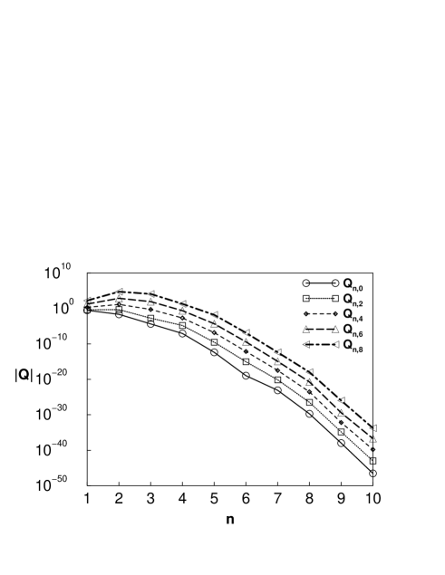
FIG. 1.: The perturbative corrections (62) to the cumulants $Q_{nj}$ plotted as a function of cycle length $n$ (for perturbation orders $j=0,2,4,6,8$) all exhibit super-exponential convergence.

The size of the cumulants is indicated in fig. 1, and the perturbative corrections to the leading eigenvalue of the weak-noise evolution operator are given in table I. Encouragingly, the value of ${\nu}_{6}=2076.47\ldots$ computed here is not wildly different to our previous numerical estimate [2] of 2700. Both the cumulants and the eigenvalue corrections exhibit a super-exponential convergence with the truncation cycle length $n$. The super-exponential convergence has been proven for the deterministic, ${\nu}_{0}$ part of the eigenvalue [7], but the proof has not been extended to the stochastic evolution operators.

We have chosen to test the formalism on this simple example, as here we are in a fortunate situation that the escape rate for arbitrary noise strength $\sigma$ can be calculated numerically by other methods to a rather high accuracy. For example, one can discretize the stochastic kernel on a spatial lattice [1] and determine numerically the leading eigenvalue.

The perturbative result in terms of periodic orbits and the weak noise corrections is compared to the eigenvalue computed by the numerical lattice discretizationin fig. 2, with the absolute difference between the numerical and the $m$th order perturbative results plotted. We see that the perturbative result ${\nu}(m,\sigma)=\sum_{k=0}^{m/2}{\nu}_{2k}\sigma^{2k}$ indeed improves as more perturbative terms are added.

FIG. 2.: The difference between the numerical and perturbative eigenvalue $|{\nu}(\sigma)-{\nu}(m,\sigma)|$. The plateau at $10^{-7}$ is a numerical artifact due to the limited accuracy of the lattice discretization calculation.

VIII Summary and outlook

In this paper we study evolution of a classical dynamical system with additive noise. In the limit of weak noise the traces of the corresponding evolution operator are approximated by sums of local traces computed on periodic orbits. Here we present a new, computationally efficient technique for evaluation of these local traces based on a matrix representation of the evolution operator, and show that method is powerful enough to enable us to compute 2 more orders of perturbation theory.

The local matrix representation can be interpreted as follows. Substituting (47) into (9) we obtain

$$\left.\mbox{\rm det}(1-z{\cal L})\right|_{\mbox{saddles}}=\prod_{p}\mbox{\rm det}(1-z^{n_{p}}{{\bf L}_{p}})\,.$$ (64)

In other words, in the saddle-point approximation the spectrum of the global evolution operator ${\cal L}$ is in this approach pieced together from the local spectra computed cycle-by-cycle on neighborhoods of individual prime cycles with periodic boundary conditions. Vattay [8] was first to formulate the $\hbar$ corrections to the semi-classical Gutzwiller theory in terms of local spectra. Here we have shown that also the stochastic flows can be suspended on the skeleton of classical periodic orbits in this way.

With so many orders of perturbation theory, we are now poised to address the issues raised by the asymptotic series nature of perturbative expansions. We can now hope to resum the series to all orders, making use of techniques such as the Borel resummation, the asymptotic expansions of general integrals of saddlepoint type, and asymptotics beyond all orders [9]. All of this is beyond the scope of the present paper, and we defer a full discussion of asymptotics to a forthcoming paper [10].

IX Acknowledgements

G.V. and G.P. gratefully acknowledges the financial support of the Hungarian Ministry of Education, FKFP 0159/1997, OMFB, OTKA T25866/F17166. G.V. thanks Bruno Eckhardt the cordial hospitalty at the Department of Physics of the Philipps-Universität Marburg and the Humboldt Fundation for support. G.P. thanks the EU network “Pattern formation, noise and spatio-temporal chaos in complex systems”, TMR contract ERBFMRXCT960085, for partial support. N.S. is supported by the Danish Research Academy Ph.D. fellowship.

$n$	${\nu}_{0}$	${\nu}_{2}$	${\nu}_{4}$	${\nu}_{6}$	${\nu}_{8}$
1	0.308	0.42	2.2	17.4	168.0
2	0.37140	1.422	32.97	1573.3	112699.9
3	0.3711096	1.43555	36.326	2072.9	189029.0
4	0.371110995255	1.435811262	36.3583777	2076.479	189298.8
5	0.371110995234863	1.43581124819737	36.35837123374	2076.4770492	189298.12802
6	0.371110995234863	1.43581124819749	36.358371233836	2076.47704933320	189298.128042526

TABLE I.: Significant digits of the leading deterministic eigenvalue ${\nu}_{0}$, and the $\sigma^{2},\cdots,\sigma^{8}$ perturbative coefficients (55), calculated from the cumulant exapansion of the spectral determinant, as a function of the cycle truncation length $n$. Note the super-exponential convergence of all coefficients.

REFERENCES

• [1] P. Cvitanović, C.P. Dettmann, R. Mainieri and G. Vattay, J. Stat. Phys. 93, 981 (1998); chao-dyn/9807034.
• [2] P. Cvitanović, C.P. Dettmann, R. Mainieri and G. Vattay, Trace formulas for stochastic evolution operators: Smooth conjugation method, submitted to Nonlinearity (November 1998); chao-dyn/9811003.
• [3] J. Bene and P. Szépfalusy, Phys. Rev. A 37, 871 (1988).
• [4] M.C. Gutzwiller, Chaos in Classical and Quantum Mechanics (Springer, New York 1990).
• [5] M. Abramowitz and I. A. Stegun, Handbook of mathematical functions with formulas, graphs and mathematical tables, Chapter 24, page 823, formula I.B, Dover, New York (1972).
• [6] P. Cvitanović, et al., Classical and Quantum Chaos, http://www.nbi.dk/ChaosBook/, (Niels Bohr Institute, Copenhagen 1999).
• [7] H.H. Rugh, Nonlinearity 5, 1237 (1992).
• [8] G. Vattay and P.E. Rosenqvist, Phys. Rev. Lett. 76, 335 (1996), chao-dyn/9509015; G. Vattay, Phys. Rev. Lett. 76, 1059 (1996).
• [9] R.B. Dingle, Asymptotic Expansions: their Derivation and Interpretation (Academic Press, London, 1973).
• [10] P. Cvitanović, C.P. Dettmann, G. Palla, N. Søndergaard and G. Vattay, Trace formulas for stochastic evolution operators: Beyond all orders, in preparation.