Structure function of passive scalars in two-dimensional turbulence

Abstract

The structure function of a scalar $\theta({\bf x},t)$, passively advected in a two-dimensional turbulent flow ${\bf u}({\bf x},t)$, is discussed by means of the fractal dimension $\delta^{(1)}_{g}$ of the passive scalar graph. A relation between $\delta^{(1)}_{g}$, the scaling exponent $\zeta_{1}^{(\theta)}$ of the scalar structure function $D_{1}^{(\theta)}(r)$, and the structure function $D_{2}(r)$ of the underlying flow field is derived. Different from the 3-d case, the 2-d structure function also depends on an additional parameter, characteristic of the driving of the passive scalar. In the enstrophy inertial subrange a mean field approximation for the velocity structure function gives a scaling of the passive scalar graph with $\delta^{(1)}_{g}<2$ for intermediate and large values of the Prandtl number $Pr$. In the energy inertial subrange a model for the energy spectrum and thus $D_{2}(r)$ gives a passive scalar graph scaling with exponent $\delta^{(1)}_{g}=\frac{5}{3}$. Finally, we discuss an application to recent observations of scalar dispersion in non-universal 2-d flows.

I Introduction

The dynamics of a scalar field $\theta({\bf x},t)$ advected in a turbulent velocity field ${\bf u}({\bf x},t)$ is of practical relevance in many fields of current research such as air pollution or chemical reactions in the stratosphere in connection with the ozone hole [1]. Especially for problems in atmospheric physics, models of two-dimensional turbulent flows give a good approximation of the dynamical processes and are frequently used[2, 3]. More recently, two-dimensional turbulence has become experimentally accessible in mercury layers[4], thin salt water layers[5, 6, 7, 8], and soap films[9, 10, 11, 12]. Two-dimensional turbulence is also interesting because of its fundamentally different behavior compared to the three-dimensional case. Since the enstrophy is a second inviscid invariant beside the energy two cascades develop: starting from a fixed, intermediate injection scale, energy is transported to larger spatial scales in an inverse energy cascade and to smaller ones in an enstrophy cascade[13, 14].

The scaling behavior of a passive scalar in a turbulent fluid was analyzed mainly in three dimensions where three different regimes could be identified. Depending on the Reynolds number of the underlying fluid turbulence and the ratio of the kinematic viscosity to the scalar diffusivity one distinguishes the viscous-convective Batchelor regime[15], the inertial-convective regime[16, 17], and the inertial-diffusive regime. In 2-d the situation is more complicated, since already the velocity field shows a variety of scaling regimes. In particular, the inverse cascade process gives rise to the formation of large scale vortices that change on very slow time scales only [18] and can dominate the dynamics of the passive scalar, at least on intermediate time scales [19, 20]. The formation of coherent vortices can be suppressed by a large scale dissipation mechanism. If this additional dissipation is present a statistically stationary homogeneous and isotropic turbulent flow field develops, that can be characterized by its structure function. We assume that a passive scalar in such a flow field also develops a statistically stationary state which can be characterized by its own structure function.

The approach used to analyse the structure function of the passive scalar is geometric measure theory [21, 22, 23, 24]. This powerful method allows to connect the structure function of the passive scalar to that of the underlying flow field and thus to link the statistical behavior of both. The result are scale resolved bounds on the scaling behavior. Upper bounds are easiest to derive and often give very good results, see e.g. the favorable comparison between theory and numerical simulations in [25]. The derivation of lower bounds is possible[23] but much more difficult and will not be attempted here. So assuming the reliability of the upper bounds we would like to see how the different regimes in ${\bf u}$ are reflected in the scaling properties of the scalar field passively advected by the flow. Some aspects of the 2-d case have been discussed previously [24], see below. In addition, we would like to compare the predictions to the results of experiments of Cardoso et al. [8], where certain discrepancies to theory were noted. As we will see the discrepancies can be accounted for if the experimentally measured structure function is substituted for the velocity field.

The model we consider is that of a scalar field $\theta({\bf x},t)$ transported in the turbulent flow field ${\bf u}({\bf x},t)$ according to

$$\frac{\partial\theta}{\partial t}+({\bf u}\cdot{\bf\nabla})\theta=\kappa{\bf\nabla}^{2}\theta+f_{\theta}\;.$$ (1)

$\kappa$ denotes the diffusivity. The force density $f_{\theta}$ models external boundary conditions and the driving and assures a statistically stationary field $\theta({\bf x},t)$. The scalar $\theta$ is assumed to be passive, i.e. it does not affect the dynamics and the statistical properties of the velocity field. We assume that in the presence of a large scale dissipation mechanism a homogeneous, isotropic, and stationary turbulent state develops. The ratio of the kinematic viscosity $\nu$ to the scalar diffusivity $\kappa$ defines the Prandtl number $Pr=\nu/\kappa$ (this is the nomenclature used when $\theta$ is a temperature field; if it describes a concentration then the corresponding ratio is known as the Schmidt number). The scaling exponents $\zeta^{(\theta)}_{n}$ of the $n$-th order scalar structure functions, defined as

$$D^{(\theta)}_{n}(r)=\langle|\theta({\bf x}+{\bf r},t)-\theta({\bf x},t)|^{n}\rangle\sim r^{\zeta^{(\theta)}_{n}}\;,$$ (2)

can be obtained from an analysis of the fractal dimension $\delta_{g}^{(d)}$ of $d$-dimensional scalar field graphs; $\langle\cdot\rangle$ denotes the statistical ensemble average. The fundamentals of the geometric measure theory approach were laid out by Constantin et al. [21, 22, 23] who derived the fractal dimension $\delta_{g}^{(d)}$ ($d$ is the space dimension). Closely related to the present investigation is the application to two-dimensional chaotic surface waves[24]. The $Pr$ dependence of 3-d passive scalar advection within this approach was discussed in [25]. As in that work we will aim at a rather direct relation between scaling exponents and velocity structure functions.

The outline of the paper is as follows. In Sec. II the basic concepts of the evaluation of the fractal graph dimension are summarized. The results of the mean-field approach[26] for fully developed two-dimensional turbulence in the direct enstrophy cascade range – the scaling behavior of the 2nd order velocity structure function $D_{2}(r)=\langle|{\bf u}({\bf x}+{\bf r},t)-{\bf u}({\bf x},t)|^{2}\rangle$ – are recalled. In a second step we interpolate the scaling of $D_{2}(r)$ to the inverse energy cascade range, where no analytical result is known. We obtain $D_{2}(r)$ from Fourier transform of an energy spectrum as is found in many numerical simulations. In Sec. III the fractal dimension of the passive scalar graph is derived over a broad range of Prandtl numbers, both in the enstrophy inertial subrange (ISR) and in the energy ISR with the previous relations for the structure function. We conclude with a summary, a discussion of the relation to the findings in the quasi-two-dimensional dispersion experiments by Cardoso et al.[8], and some remarks on open questions.

II Basic concepts

A Fractal dimension of the passive scalar graph

From now on all considerations are made for the case of a two-dimensional flow field. The graph of the scalar field is then a 2-d surface in 3-d space. The Hausdorff dimension of this graph is obtained from the scaling behavior of the Hausdorff volume $H(G(B_{r}^{(2)}))$ of the graph $G(B_{r}^{(2)})=\{({\bf x},\theta)|{\bf x}\in B_{r}^{(2)},\,\theta=\theta({\bf x})\}$ over a disk of radius $r$ (the 2-d ball $B_{r}^{(2)}$) [27],

$$H(G(B_{r}^{(2)}))\sim r^{\delta_{g}^{(2)}}\;.$$ (3)

In two dimensions the fractal dimension $\delta_{g}^{(2)}$ is connected to the scaling exponent $\zeta^{(\theta)}_{1}$, cf. eq. (2), through the inequality[22]

$$\delta_{g}^{(2)}\leq 3-\zeta^{(\theta)}_{1}\;.$$ (4)

We assume equality in (4)[22, 25] and use the relation $\delta_{g}^{(1)}=\delta_{g}^{(2)}-1$, where $\delta_{g}^{(1)}$ is the fractal dimension of the level sets $\theta_{0}=\theta({\bf x})$. The relative Hausdorff volume $H(G(B_{r}^{(2)}))/V(B_{r}^{(2)})$ is given by geometric measure theory[28, 29] as

$$\frac{H(G(B_{r}^{(2)}))}{V(B_{r}^{(2)})} = \frac{1}{V(B_{r}^{(2)})}\int_{B_{r}^{(2)}}\,\sqrt{1+r^{2}|{\bf\nabla}\tilde{\theta}|^{2}}\,\mbox{d}^{2}{\bf x}\;,$$ (5)

$$\leq \sqrt{1+\frac{1}{\pi}\int_{B_{r}^{(2)}}\,|{\bf\nabla}\tilde{\theta}|^{2}\,\mbox{d}^{2}{\bf x}}\;,$$ (6)

where the Cauchy-Schwartz inequality and $V(B_{r}^{(2)})=\pi\,r^{2}$ were used in the last line. The passive scalar field $\theta({\bf x},t)$ is measured in units of $\theta_{r.m.s.}=\sqrt{\langle\theta^{2}\rangle}$, thus leading to dimensionless $\tilde{\theta}=\theta/\theta_{r.m.s.}$. Equation (5) is a generalization of the well-known volume formula $V=\int\sqrt{g}\,\mbox{d}^{2}{\bf y}$ to fractal sets, where $V$ is a two-dimensional curved hyper surface embedded in the three-dimensional Euclidean space and $g$ the determinant of the metric tensor $g_{ij}(y^{1},y^{2})$.

We now turn to the evaluation of $\delta_{g}^{(2)}$. The term $|{\bf\nabla}\tilde{\theta}|^{2}$ can be replaced by means of (1) by

$$|{\bf\nabla}\tilde{\theta}|^{2}=\frac{1}{2\kappa}(\kappa\Delta\tilde{\theta}^{2}-({\bf u}\cdot{\bf\nabla})\tilde{\theta}^{2})+\frac{f_{\theta}\tilde{\theta}}{\kappa\theta_{r.m.s.}}\;.$$ (7)

With this eq. (5) becomes

$$\frac{H(G(B_{r}^{(2)}))}{V(B_{r}^{(2)})}\leq\sqrt{1+\frac{1}{\pi}\int_{B_{r}^{(2)}}\,\left\{\frac{1}{2\kappa}[-({\bf u}\cdot{\bf\nabla})\tilde{\theta}^{2}+\kappa\Delta\tilde{\theta}^{2}]+\frac{f_{\theta}\tilde{\theta}}{\kappa\theta_{r.m.s.}}\right\}\,\mbox{d}^{2}{\bf x}}\;.$$ (8)

We will consider the three integrals under the square root separately and denote them by $I_{1}$, $I_{2}$, and $I_{3}$, respectively. In the three-dimensional case[25] the terms $I_{2}$ and $I_{3}$ vanish in the large Reynolds number limit. They also satisfy the inequality $I_{2}\leq 3\sqrt{I_{3}}$ which changes to $I_{2}\leq 2\sqrt{I_{3}}$ in the two-dimensional case. $I_{3}$ can be estimated as

$$I_{3}=\frac{1}{\pi}\int_{B_{r}^{(2)}}\,\frac{f_{\theta}\tilde{\theta}}{\kappa\theta_{r.m.s.}}\,\mbox{d}^{2}{\bf x}=\frac{r^{2}\epsilon_{\theta}}{\kappa\theta_{r.m.s.}^{2}}=\frac{\epsilon_{\theta}\epsilon_{\omega}^{-1/3}}{\theta_{r.m.s.}^{2}}Pr\,\tilde{r}^{2}\;,$$ (9)

where the scalar dissipation rate $\epsilon_{\theta}=\kappa\langle|{\bf\nabla}\theta|^{2}\rangle$, the enstrophy dissipation rate $\epsilon_{\omega}=\nu\langle|{\boldmath\nabla}\omega|^{2}\rangle$, and stationarity are used. In the case of a three-dimensional passive scalar this term contains a factor $\nu^{1/2}$ and thus can be neglected. In 2-d the smallest scales are given by the enstrophy dissipation rate and this factor disappears. Hence $I_{3}$ cannot be neglected; its importance is evidently controlled by Prandtl number $Pr$, length scale $r$ and dimensionless prefactor

$$\alpha=\frac{\epsilon_{\theta}\epsilon_{\omega}^{-1/3}}{\theta_{r.m.s.}^{2}}\,.$$ (10)

The term $I_{2}$ can still be neglected on account of its subdominant scaling in $r$. We introduce dimensionless length scales $\tilde{r}=r/\eta_{\omega}$ by means of the enstrophy dissipation length $\eta_{\omega}=\nu^{1/2}\epsilon_{\omega}^{-1/6}$ since in 2-d turbulence it is the enstrophy cascade that brings the energy to the smallest scales where viscosity dominates.

It follows from (8) for $I_{1}$ by applying the Gauss Theorem and the Cauchy-Schwarz inequality

$$I_{1} = \frac{r}{\kappa}\oint_{\partial B_{r}^{(2)}}\frac{\tilde{\theta}^{2}({\bf u}-{\bf u}_{0})\cdot{\bf n}}{u_{r}}\,\mbox{d}\,r\;,$$ (11)

$$\leq \frac{r}{\kappa}\sqrt{\oint_{\partial B_{r}^{(2)}}\frac{\tilde{\theta}^{4}}{u_{r}}\,\mbox{d}\,r}\;\sqrt{\oint_{\partial B_{r}^{(2)}}\frac{(({\bf u}-{\bf u}_{0})\cdot{\bf n})^{2}}{u_{r}}\,\mbox{d}\,r}\;.$$ (12)

The quantity $u_{r}=2\pi r$ is the circumference. It is possible to add ${\bf u}_{0}$, the velocity at the center of $B_{r}^{(2)}$, due to the assumed homogeneity.

The first term on the right hand side contains the square root of the passive scalar flatness. Since we are interested in the scaling properties of $I_{1}$, it suffices to know that the scalar flatness is a constant, independent of $r$. However, there do not seem to be numerical or experimental data for the passive scalar flatness in 2-d. Data for the velocity field from the experiments [6] and the numerical simulations [30] suggest Gaussian behavior in the absence of coherent structures in the regime of the inverse cascade. More recent experiments suggest that this result also extends into the region of the direct enstrophy cascade [31]. However, since there are models where a Gaussian statistics for a random velocity field causes non-Gaussian scalar statistics [32, 33], this information is insufficient to infer Gaussian statistics for the passive scalar. In the following we will work with the Gaussian flatness value of three for the passive scalar. It should be kept in mind that deviations from this value will most likely be scale dependent and will give rise to modifications of the scaling exponents.

The second term is the longitudinal velocity structure function $D_{\parallel}(r)$. Thus we find

$$I_{1}\leq\frac{\sqrt{3}}{\kappa}r\sqrt{D_{\parallel}(r)}\;.$$ (13)

Combining (3), (8), (9), and (13) we end up with an inequality for the fractal dimension $\delta^{(2)}_{g}$ of the passive scalar graph in two dimensions,

$$\delta^{(2)}_{g}-2\leq\frac{\mbox{d}}{\mbox{d}\,\ln\tilde{r}}\ln\sqrt{1+\frac{\epsilon_{\theta}\epsilon_{\omega}^{-1/3}}{\theta_{r.m.s.}^{2}}Pr\,\tilde{r}^{2}+\sqrt{3}Pr\tilde{r}\sqrt{\tilde{D_{\parallel}}}}\;,$$ (14)

where $\tilde{D}_{\parallel}=D_{\parallel}/(\epsilon^{2/3}_{\omega}\eta_{\omega}^{2})$. This inequality, relating the scaling exponent $\delta^{(2)}_{g}$ to the longitudinal structure function of the underlying turbulent flow field $\tilde{D_{\parallel}}$ is the main result of this section. For most of the discussion that follows we will assume equality in (14); in the three-dimensional case this is a very good assumption [25].

B Structure functions in two-dimensional turbulence

To evaluate (14) we need information on the scaling behavior of the 2nd order longitudinal structure function $D_{\parallel}$. The longitudinal structure function $D_{\parallel}(r)$ and transversal structure function $D_{\perp}(r)$ make up the velocity structure function $D_{2}(r)$ and are connected by incompressibility, $D_{\perp}=D_{\parallel}+r\frac{dD_{\parallel}}{dr}$. Eliminating the transversal part then gives [34, 35]

$$D_{\parallel}(r)=\frac{1}{r^{2}}\int_{0}^{r}\rho\,D_{2}(\rho)\,\mbox{d}\,\rho\;.$$ (15)

As there are two inertial ranges with several different scaling regimes, there is no analytical expression for the structure function. As far as we are aware, the best that can be achieved analytically is the structure function for the enstrophy cascade as discussed by Grossmann and Mertens[26]. They used a mean field type approach for the fully developed, turbulent velocity field in the enstrophy cascade, i.e. for spatial scales $\eta_{\omega}<r<r_{in}$. Separating small and large scales one finds energy and enstrophy balance equations where terms resulting from the small scale fluctuations act like an effective eddy viscosity for the large scale components of $\omega$. Analytical expressions for the 2nd order vorticity structure function $D^{(\omega)}_{2}(r)$ and the 2nd order velocity structure function $D_{2}(r)$ can be found using the Batchelor interpolation technique[26, 36]. In dimensionless form they read

$$\tilde{D}_{2}(\tilde{r}) = \frac{\tilde{D}_{2}^{(\omega)}(\infty)}{4}\,\frac{\tilde{r}^{2}}{(1+a\,\tilde{r}^{2})^{1/3}}+\left(\frac{Re^{\ast}}{2}-\frac{\tilde{D}_{2}^{(\omega)}(\infty)}{4}\right)\,\tilde{r}^{2}\;,$$ (16)

with the parameter $a=\frac{15}{592}$ and the asymptotic value $\tilde{D}^{(\omega)}_{2}(\infty)=D^{(\omega)}_{2}(\infty)/\epsilon_{\omega}^{2/3}=14.8$. This spectrum also depends on the energy dissipation $\epsilon$, which when expressed in the length and energy scales of the enstrophy cascade becomes the dimensionless parameter $Re^{\ast}=\epsilon/(\epsilon_{\omega}^{2/3}\nu)$. The structure functions are shown in Fig. 1. Besides the prominent $\tilde{r}^{2}$ behavior that follows already by dimensional analysis one notes an intermediate scaling with $\tilde{r}^{4/3}$; the range over which this scaling is observed depends on $Re^{\ast}$ (see below). The corresponding longitudinal velocity structure function $\tilde{D}_{\parallel}(\tilde{r})$ is given with eq. (15) by

$$\tilde{D}_{\parallel}(\tilde{r}) = \left(\frac{Re^{\ast}}{8}-\frac{\tilde{D}_{2}^{(\omega)}(\infty)}{16}\right)\,\tilde{r}^{2}+\frac{3\tilde{D}_{2}^{(\omega)}(\infty)}{8a}$$ (17)

$$\times \left[\frac{(1+a\,\tilde{r}^{2})^{5/3}-1}{5\,a\,\tilde{r}^{2}}-\frac{(1+a\,\tilde{r}^{2})^{2/3}-1}{2\,a\,\tilde{r}^{2}}\right]\;.$$ (18)

For the energy ISR no such analytical expression is known. We therefore combine a model for the energy distribution in $k$-space with numerical transformations to obtain the longitudinal structure function. Recent experiments on forced two-dimensional turbulence[6, 12], a number of direct numerical simulations[30, 37, 38, 39, 40, 41], field theoretical investigations[42] as well as cascade models[43] support the existence of a Kolmogorov-like scaling for the energy spectrum, $E(k)\sim\,k^{-5/3}$ for $(k<k_{f})$, in the energy ISR and $E(k)\sim\,k^{-\beta}$ with $\beta\geq 3$ for $(k>k_{f})$ for the enstrophy ISR. We therefore start with the following model spectrum for the amplitudes $\langle|{\bf u}_{\bf k}|^{2}\rangle$ of the velocity field in a Fourier representation in a periodic box of size $L=2\pi$

$$\langle|{\bf u}_{\bf k}|^{2}\rangle\!\sim\!\left\{\begin{array}[]{r@{\quad:\quad}l}k^{3}&\frac{2\pi}{L}\leq k\leq k_{1},\\ k^{-2/3}&k_{1}<k\leq k_{f},\\ k^{-\beta}&k_{f}<k\leq k_{\omega}=\frac{1}{\eta_{\omega}},\;\beta\geq 2\,,\\ k^{-\beta}\exp\left[-\left(\frac{k-k_{\omega}}{k_{\omega}}\right)^{2}\right]&k_{\omega}<k\;.\end{array}\right.$$ (23)

Note the different scalings for $\langle|{\bf u}_{\bf k}|^{2}\rangle$ and the energy spectrum $E(k)$ due to phase space factor, i.e. $E(k)\!\sim\!k^{-\beta-1}$ corresponds to $\langle|{\bf u}_{\bf k}|^{2}\rangle\!\sim\!k^{-\beta}$.

The first range approximates finite system size effects where we have chosen a slope of 3 in correspondence with results of numerical experiments[37, 41]. This is followed by the inverse energy cascade range with a Kolmogorov-like scaling law. At the injection scale $k_{f}$ the enstrophy cascade to larger values of $k$ starts, followed by the viscous cutoff. The energy spectra with $\beta=3$ for three different values of the injection wavenumber $k_{f}$ are shown in Fig. 2.

The relation between velocity spectrum scaling and the velocity structure function $D_{2}(r)$ assuming stationarity, homogeneity, and isotropy is given by the volume average

$$D_{2}(r) = \frac{1}{V}\int_{V}\,|\,{\bf u}({\bf x}+{\bf r})-{\bf u}({\bf x})\,|^{2}\,\mbox{d}\!V,$$ (24)

$$= \frac{1}{V}\int_{V}\,|\,\sum_{{\bf k}}{\bf u}_{\bf k}\,\exp(i{\bf k}\cdot{\bf x})[\exp(i{\bf k}\cdot{\bf r})-1]\,|^{2}\,\mbox{d}\!V,$$ (25)

$$= 2\,\sum_{{\bf k}}\,\langle|{\bf u}_{\bf k}|^{2}\rangle\,(1-\cos{({\bf k}\cdot{\bf r})})\,.$$ (26)

By averaging over all directions (due to isotropy) in ${\bf k}$-space the cosine gives rise to the Bessel function $\mbox{J}_{0}(kr)$,

$$D_{2}(r)=2\,\sum_{k}\,\langle|{\bf u}_{\bf k}|^{2}\rangle\,(1-\mbox{J}_{0}(kr))\,.$$ (27)

The model spectrum (23) is then substituted and the summation in (27) is evaluated numerically using a finite, geometrically scaling set of wave numbers. It should be mentioned here that the model does not contain a spectral range that would correspond to the intermediate $\tilde{r}^{4/3}$–scaling of the structure function in the enstrophy ISR found in the analytical theory. We will come back to this point in the discussion of our results.

III Results

A Fractal dimension in the enstrophy ISR

We first calculate the scaling behavior in the enstrophy ISR where the analytical expression (16) is available. Inserting (16) in (14) and neglecting the term $I_{3}$ for the moment, one notes that $\delta_{g}^{(2)}$ depends on three quantities: the parameter $Re^{\ast}$, the Prandtl number $Pr$, and the scale $\tilde{r}$ itself. The numerical result for $\delta_{g}^{(1)}=\delta_{g}^{(2)}-1$ are shown in Fig. 3 for a Prandtl number range varying over ten orders of magnitude and $Re^{\ast}=7.6$. The grey shaded area denotes the range of scales where $\tilde{r}^{4/3}$ gives the main contribution to the structure function. It is only in this range that we find $1<\delta_{g}^{(1)}<2$. The range is bounded by $\tilde{r}_{1}\leq\tilde{r}\leq\tilde{r}_{2}$ where $\tilde{r}_{1}$ is the crossover scale from the viscous subrange (VSR) and $\tilde{r}_{2}$ is the crossover scale to the $\tilde{r}^{2}$–scaling in the enstrophy ISR,

$$\tilde{r}_{1} = \frac{1}{\sqrt{3}}(\tilde{D}_{2}^{(\omega)}(\infty))^{2}(Re^{\ast})^{-3/2}\;,$$ (28)

$$\tilde{r}_{2} = \frac{1}{\sqrt{3}}(\tilde{D}_{2}^{(\omega)}(\infty))^{2}(Re^{\ast}-\tilde{D}_{2}^{(\omega)}(\infty)/2)^{-3/2}\;,$$ (29)

where $\tilde{D}_{2}^{(\omega)}(\infty)=14.8$ has to be taken. The larger $Re^{\ast}$ the smaller the range of the $\tilde{r}^{4/3}$–scaling. It can be observed only for $Re^{\ast}$ within the interval

$$7.4\!\approx\!\frac{\tilde{D}_{2}^{(\omega)}(\infty)}{2}\leq Re^{\ast}\leq\left(\frac{(\tilde{D}_{2}^{(\omega)}(\infty))^{4}}{3}\right)^{1/3}\!\approx\!25\;.$$ (30)

The lower bound follows from the positivity of the structure function by its definition (cf. second term of (16)). The upper bound is a result of eq. (28) and the constraint $\tilde{r}_{1}\geq 1$. For $Re^{\ast}$ approaching 7.4 follows $\tilde{r}_{2}$ goes to infinity. The $\tilde{r}^{4/3}$– scaling range is then extended over the whole enstrophy ISR. We see in Fig. 4 that for increasing $Re^{\ast}$ the intermediate fractal scaling of the graph is more and more suppressed and conclude that this behavior of $\delta^{(1)}_{g}$ is due to the presence of the $\tilde{r}^{4/3}$–scaling range. The above estimates give $\tilde{r}_{1}\!\approx\!6.0$ and $\tilde{r}_{2}\!\approx\!1400$ for $Re^{\ast}=7.6$ and $\tilde{r}_{1}\!\approx\!1.0$ and $\tilde{r}_{2}\!\approx\!1.7$ for $Re^{\ast}=25.0$, respectively. In the lower panel the corresponding scaling exponent of the scalar structure function $\zeta^{(\theta)}_{1}=2-\delta^{(1)}_{g}$ is plotted. The plateau of the structure function $D_{1}^{(\theta)}$ for large Prandtl number and scales below the smallest scales in the turbulent fluid ($r/\eta_{\omega}<1$) corresponds to the Batchelor regime of chaotic scalar advection in a smooth fluid[15].

For small values of $Pr$ the diffusion $\kappa$ dominates the passive scalar dynamics. The scalar field is smooth, $\delta^{(1)}_{g}=1$. The exponent $\delta^{(1)}_{g}$ grows when the second term in the square root of eq. (14) becomes dominant. By inserting the power law $\tilde{D}_{\parallel}=\frac{\sqrt[3]{9}}{20}(\tilde{D}_{2}^{(\omega)}(\infty)\tilde{r})^{4/3}$ for the enstrophy ISR at $\tilde{r}=\tilde{r}_{c}$ one gets a crossover for

$$\tilde{r}_{c}=\sqrt[10]{\frac{8000}{243}}Pr^{-3/5}(\tilde{D}_{2}^{(\omega)}(\infty))^{-2/5}\approx 0.48\,Pr^{-3/5}.$$ (31)

By putting $\tilde{r}_{c}=\tilde{r}_{2}$ and using (28) the maximum Prandtl number $Pr_{s}$ without fractal $\delta^{(1)}_{g}$ can be estimated as

$$Pr_{s}<2\sqrt{5}(\tilde{D}_{2}^{(\omega)}(\infty))^{-4}(Re^{\ast}-\tilde{D}_{2}^{(\omega)}(\infty)/2)^{5/2}\;.$$ (32)

With $Re^{\ast}=7.6$ and $25.0$ this gives $Pr_{s}\lesssim 2\cdot 10^{-6}$ and $10^{-1}$, respectively.

For large values of $Pr$ one observes a transition to $\delta^{(1)}_{g}=2$ even when the velocity field is in the VSR. Again the second term of (14) dominates because of its large prefactor $Pr$. Taking $\tilde{D}_{\parallel}=\frac{Re^{\ast}}{8}\tilde{r}^{2}$ for the VSR gives

$$\tilde{r}_{c}=\sqrt[4]{\frac{8}{3}}Pr^{-1/2}(Re^{\ast})^{-1/4}\;.$$ (33)

With $\tilde{r}_{c}=\frac{1}{10}\tilde{r}_{1}$ we get those $Pr_{l}$ which give $\delta^{(1)}_{g}=2$ in the VSR over at least one decade of scales,

$$Pr_{l}>200\sqrt{6}(\tilde{D}_{2}^{(\omega)}(\infty))^{-4}(Re^{\ast})^{5/2}\;.$$ (34)

For $Re^{\ast}=7.6$ and $25.0$ this results in $Pr_{l}\!\gtrsim\!2.0$ and $30.0$, respectively.

The structure function of a passive scalar in the enstrophy ISR shows four different regimes. For very small $\tilde{r}$ smoothness gives $\delta_{g}^{(1)}=1$. This is followed by the Batchelor regime $\delta_{g}^{(1)}=2$ for sufficiently large $Pr$. The $\tilde{r}^{4/3}$–scaling discovered by Grossmann and Mertens is reflected in a decrease of $\delta_{g}^{(1)}$ below $2$ near $r/\eta_{\omega}\approx 10^{1\pm 1}$. For larger $\tilde{r}$ it goes back up to $2$.

So far we neglected the term $I_{3}=\alpha\,Pr\,\tilde{r}^{2}$ (see (9) and (10)) in our calculation. Because of its $\tilde{r}^{2}$-scaling it dominates the structure function for large $\tilde{r}$. In [24] this term was assumed to be subdominant. Substituting the various definitions it can be expressed as a ratio of two rates,

$$\alpha=\frac{\kappa\langle|{\bf\nabla}\theta|^{2}\rangle}{(\nu\langle|{\bf\nabla}\omega|^{2}\rangle)^{1/3}\langle\theta^{2}\rangle}=\frac{r_{\theta}}{r_{\omega}}\,.$$ (35)

The rate $r_{\theta}=\epsilon_{\theta}/\theta^{2}_{r.m.s.}$ is a scalar forcing rate. $r_{\omega}=\epsilon_{\omega}^{1/3}$ is the strain rate in the enstrophy cascade and characteristic of the passive scalar advection by the vortices. The case $\alpha>1$ then corresponds to $r_{\theta}>r_{\omega}$, i.e. fast driving and slow advection. Then the scalar field fills space and $\delta_{g}^{(1)}\sim 2$. In the other case, $\alpha<1$, the advection dominates and the structure function of the fluid is reflected in that of the scalar. It is this latter case that was discussed in [24] for surface waves. The size of $\alpha$ is determined by the experimental situation and has to be taken from measurements. All quantities that enter (35) are experimentally accessible; note that the enstrophy dissipation rate is related to velocity gradients via $\epsilon_{\omega}=-8\langle(\partial_{x}u_{x})^{3}\rangle$[26].

Results for different $Pr$ with $\alpha=1$ are shown in Fig. 5. The main effect of an increasing $I_{3}$ is the suppression of the crossover scaling and a transition for large $r$.

B Extension to the energy ISR

The extension of $D_{2}(r)$ to the whole range of scales is done with (27) and the results for $\delta_{g}^{(1)}$ are given in Fig. 6 for three input model spectra (see Fig. 2) which differ by the injection wavenumber $k_{f}$. The smaller $k_{f}$ the longer is the enstrophy ISR extended which results in a dominant range where $\delta_{g}^{(1)}=2$. On the other hand, the larger $k_{f}$ the more dominant the inverse energy cascade range, indicated as the grey shaded area in Fig. 6. The corresponding longitudinal velocity structure function $D_{\parallel}(r)$ is superimposed. Note that the model spectrum has to be normalized to give $\tilde{D}_{\parallel}=\frac{Re^{\ast}}{8}\tilde{r}^{2}$ in the VSR. In the enstrophy ISR we find $\tilde{D}_{\parallel}(r)\sim\tilde{r}^{2}$ and in the energy ISR $\tilde{D}_{\parallel}(r)\sim\tilde{r}^{2/3}$, leading to $\delta_{g}^{(1)}=2$ and $\delta_{g}^{(1)}=\frac{5}{3}$, respectively. As mentioned, the model spectrum does not show the $\tilde{r}^{4/3}$–scaling predicted by [26]. Therefore, if $Re^{\ast}$ is in the range where a $\tilde{r}^{4/3}$–scaling appears the $\delta_{g}^{(1)}$ values for $r\simeq\eta_{\omega}$ have to be replaced by the ones in Figs. 3, 4, and 5. For very large values of $r$ we can replace $\mbox{J}_{0}(kr)$ by its asymptotic form $\mbox{J}_{0}(kr)\approx\sqrt{\frac{2}{\pi kr}}\cos(kr-\frac{\pi}{4})$ resulting in $D_{2}(r)\approx 2\,\sum_{k}\,\langle|{\bf u}_{\bf k}|^{2}\rangle$ in (27). The constant asymptotic behavior of the structure function corresponds with $\delta_{g}^{(1)}=\frac{3}{2}$ (cf. (14)).

The model spectrum contains a free parameter $\beta$ which has no agreed upon value. Numerical simulations [38, 39, 40, 41] suggest a range $\beta\in[2,4]$. For $\beta=2$ we get $\delta_{g}^{(1)}$ slightly below 2 in the enstrophy ISR which changes clearly to $\delta_{g}^{(1)}=2$ for $\beta>2$ (cf. Fig. 7). As expected, the value of $\delta_{g}^{(1)}$ in the energy ISR is insensitive to a $\beta$–variation.

Again we have to discuss the additional influence of the $I_{3}$ term in (8). Will inverse cascade effects be suppressed in the large $Pr$ number case because of the dominance of the $\tilde{r}^{2}$–scaling at large separations? In order to determine the scale $\tilde{r}_{c}$ where $I_{3}\geq I_{1}$, we use the experimental value for the Kolmogorov constant $C_{K}$ [6] and assume a completely extended inverse cascade with no intermittency corrections. Then $D_{2}(r)=4\,C_{K}\,\epsilon^{2/3}\int^{\infty}_{0}(1-\mbox{J}_{0}(kr))k^{-5/3}\,\mbox{d}\,k$ and $\tilde{D_{2}}=b_{2}\tilde{r}^{2/3}$. With $C_{K}$ between 5.5 and 7, we find $b_{2}$ between 31.5 and 40 for the energy ISR and thus finally

$$\tilde{r}_{\alpha}\geq\left(\frac{9b_{2}}{8\alpha^{2}}\right)^{3/4}\approx l\alpha^{-3/2}\;,$$ (36)

where $l$ lies between 14 and 17. The scale $\tilde{r}_{\alpha}$ is shifted towards larger values for decreasing $\alpha$. A factor $\alpha\!\sim\!1$ can suppress the scaling behavior in the energy ISR which was found above completely. This fact is illustrated in Fig. 8. Clearly the asymptotic state for $\tilde{r}$ to infinity leads here to $\delta_{g}^{(1)}$ approaching 2.

IV DISCUSSION

Our main findings for a passive scalar in a 2-d turbulent flow field can be summarized as follows: (1) There is a critical scale set by equation (31) below which the spectrum is smooth, $\delta_{g}^{(1)}=1$, because of diffusion dominance. (2) Between this scale and the injection scale $r_{in}$ the scaling exponent $\delta_{g}^{(1)}=2$ in most cases. (3) An exception is found for $Re^{*}$ in the interval set by (30), where a scaling exponent $\delta_{g}^{(1)}<2$ is found. The limits of this interval are given by (28) and the deviation from 2 is controlled by the parameter $\alpha$, eq. (35). (4) Beyond the injection length and up to a length set by equation (36), the scalar field scales with the exponent $\delta_{g}^{(1)}=5/3$ as expected for the energy inertial subrange. (5) Above the length scale set by (36), the exponent again increases to $2$. What is most surprising is that the scaling derived within geometric measure theory depends not only on the scaling of the velocity field but also on two additional dimensionless numbers, the Reynolds number $Re^{*}$ which causes the intermediate scaling in the enstrophy viscous subrange and on $\alpha$ which suppresses the velocity field induced scaling at large separations for rapid driving.

At this point input from experiments on two-dimensional turbulence is necessary to check and expand the theoretical results. Cardoso et al. [8] measured dispersion in a quasi-two-dimensional turbulent flow and compared with results for the energy inertial subrange. They observed a velocity structure function with scaling $\tilde{r}^{0}$ and a fractal dimension $\delta_{g}^{(1)}$ between $1.3$ and $1.5$ with an average of about $1.4$. Substituting a velocity scaling function $\tilde{D}_{\parallel}=C\tilde{r}^{0}$ in our main equation (14) gives

$$\delta^{(1)}_{g}\leq 1+\frac{\mbox{d}}{\mbox{d}\,\ln\tilde{r}}\ln\sqrt{1+5000(\alpha\tilde{r}^{2}+\sqrt{3C}\tilde{r})}\;.$$ (37)

If the quadratic term can be neglected, i.e. if $\tilde{r}$ is small enough, the inequality reads $\delta^{(1)}_{g}\leq 3/2$. The experimental results are indeed below but close to this limit, so that the assumption that the distances are small is probably reasonable. For larger separation there is a crossover to $\delta^{(1)}_{g}\leq 2$, and it would be interesting to see whether the experimental data follow this behavior. For the energy inertial subrange [and not too large separations, see (36)], the inequality would be $\delta^{(1)}_{g}\leq 5/3$, higher than the one for the experimentally observed spectrum.

Further experiments or numerical studies to check the results from geometric measure theory, especially the ones for the enstrophy cascade and for the dependence on $\alpha$, are clearly needed. Perhaps it is possible to combine the experiments on passive scalar mixing [8, 7] with the set-up for extended, stationary inverse and direct cascades [6, 31] in order to measure the scaling behavior mentioned in (2). In order to check the predictions for the enstrophy cascade in (1) the spatial resolution has to be enlarged. Otherwise e.g. the existence of the intermediate $\tilde{r}^{4/3}$–scaling of $\tilde{D}_{2}(\tilde{r})$ cannot be detected. We remind the reader that this range is only well established for values of $Re^{\ast}$ close to its lower threshold (see Fig. 1). Its localization with respect to $\tilde{r}$ prevents it from being seen in the Fourier spectrum, as already discussed by Grossmann and Mertens [26].

Another open question which calls for more input from numerical simulations and experiments is that of the scalar flatness in 2-d. For a non-Gaussian scalar statistics we would expect a scale–dependent flatness $F_{\theta}(\tilde{r})$ causing a further scale dependence of the third term in (14) and thus leading to a modification of the present model.

The problem studied here has also interesting links to magnetohydrodynamics. First steps towards using geometric measure theory in this context were undertaken by Grauer and Marliani[44]. In two dimensions there is a direct relation between magnetic field advection and the scalar dynamics studied here since the vector potential for the magnetic field has only a $z$-component. Consequences of this relation are under investigation.

FIG. 1.: Velocity structure function $D_{2}(r)$ in the enstrophy inertial subrange for four different values of $Re^{\ast}$.

FIG. 2.: Model spectrum $\langle|{\bf u}_{\bf k}|^{2}\rangle$ for three different values of $\tilde{k}_{f}$ indicated by the arrows ($\tilde{k}_{f}\approx 2\cdot 10^{-5},5\cdot 10^{-4},10^{-2}$). The wavenumbers are given in units of $k_{\omega}=\eta_{\omega}^{-1}.$ The exponent $\beta$ was set to three.

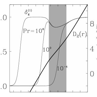
FIG. 3.: Fractal dimension $\delta_{g}^{(1)}$ for three Prandtl numbers and the corresponding velocity structure function $\tilde{D_{2}}(\tilde{r})$ (thick line) for $Re^{\ast}=7.6$. The grey shaded area denotes the range of scales where the $\tilde{r}^{4/3}$ term dominates for the parameter set. A fractal $\delta_{g}^{(1)}$ can be observed in this range of scales.

FIG. 4.: Fractal dimension $\delta_{g}^{(1)}$ and scaling exponent $\zeta^{(\theta)}_{1}$ as a function of $Pr=10^{\lambda}$ and of $Re^{\ast}$. The solid line is $Re^{\ast}=7.4$ (the lower bound), the dotted line is $Re^{\ast}=7.6$, and the dashed line is $Re^{\ast}=13.0$ in both panels. Note that $\zeta^{(\theta)}_{1}=2-\delta_{g}^{(1)}$.

FIG. 5.: Fractal dimension $\delta_{g}^{(1)}$ as a function of $Pr=10^{\lambda}$ for $Re^{\ast}=7.6$, $\alpha=1$. The solid line plots show the results when only the advection term $I_{1}$ is taken. The dotted lines show the additional influence of the forcing term $I_{3}$.

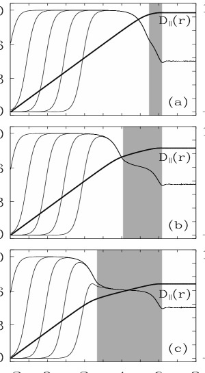
FIG. 6.: Longitudinal velocity structure function $\tilde{D}_{\parallel}(\tilde{r})$ (thick line) and fractal dimension $\delta^{(1)}_{g}$ over $\tilde{r}$ for $Re^{\ast}=7.6$ and $Pr=10^{4},10^{2},10^{0},10^{-2}$, and $10^{-4}$ decreasing from left to right. The grey shaded range of scales denotes the inverse energy cascade range of $\langle|{\bf u}_{\bf k}|^{2}\rangle$. (a): $\tilde{k}_{f}\approx 2\cdot 10^{-5}$, (b): $\tilde{k}_{f}\approx 5\cdot 10^{-4}$, (c): $\tilde{k}_{f}\approx 10^{-2}$. The exponent $\beta=3$ was taken.

FIG. 7.: Fractal dimension $\delta_{g}^{(1)}$ for $Pr=10^{4}$ and $Re^{\ast}=7.6$ for different values of the scaling exponent $\beta$ taken in the enstrophy ISR for the model spectrum $\langle|{\bf u}_{\bf k}|^{2}\rangle$ (cf. (23)).

FIG. 8.: Fractal dimension $\delta_{g}^{(1)}$ for $Re^{\ast}=7.6$ and for three different values of the parameter $\alpha=\epsilon_{\theta}\epsilon_{\omega}^{-1/3}/\theta_{r.m.s.}^{2}$. The exponent $\beta=3$ was taken.

REFERENCES

- [1] S. Edouard, B. Legras, F. Levèvre, and R. Eymard, Nature 384, 444 (1996).
- [2] D. K. Lilly, J. Atmos. Sci. 46, 2026 (1989).
- [3] M. Lesieur, Turbulence in Fluids, (Martinus Nijhoff Publishers, Dodrecht) 1987.
- [4] J. Sommeria, J. Fluid Mech. 170, 139 (1986).
- [5] P.Tabeling, S. Burkhart, O. Cardoso, and H. Willaime, Phys. Rev. Lett. 67, 3772 (1991).
- [6] J. Paret and P.Tabeling, Phys. Rev. Lett. 79, 4162 (1997).
- [7] B. S. Williams, D. Marteau, and J. P. Gollub, Phys. Fluids 9, 2061 (1997).
- [8] O. Cardoso, B. Gluckmann, O. Parcollet, and P.Tabeling, Phys. Fluids 8, 209 (1996).
- [9] M. Gharib and P. Derango, Physica D 37, 406 (1989).
- [10] B. K. Martin, X. L. Wu, W. I. Goldburg, and M. A. Rutgers, Phys. Rev. Lett. 80, 3964 (1998).
- [11] M. Rivera, P. Vorobieff, and R. E. Ecke, Phys. Rev. Lett. 81, 1417 (1998).
- [12] M. A. Rutgers, Phys. Rev. Lett. 81, 2244 (1998).
- [13] R. H. Kraichnan, Phys. Fluids 10, 1417 (1967).
- [14] G. K. Batchelor, Phys. Fluids Supplement 2, 233 (1969).
- [15] G. K. Batchelor, J. Fluid Mech. 5, 113 (1959).
- [16] A. M. Obukhov, Izv. Akad. Nauk SSSR, Ser. Geog. Geofiz. 13, 58 (1949).
- [17] S. Corrsin, J. Appl. Phys. 22, 469 (1951).
- [18] R. Benzi, S. Patarnello, and P. Santangelo, Europhys. Lett. 3, 811 (1987).
- [19] A. Babiano, C. Basdevant, B. Legras, and R. Sadourny, J. Fluid Mech. 183, 379 (1987).
- [20] C. Basdevant and T. Philipovitch, Physica D 37, 17 (1994).
- [21] P. Constantin, I. Procaccia, and K. R. Sreenivasan, Phys. Rev. Lett. 67, 1739 (1991).
- [22] P. Constantin and I. Procaccia, Phys. Rev. E 47, 3307 (1993).
- [23] P. Constantin and I. Procaccia, Nonlinearity 7, 1045 (1994).
- [24] I. Procaccia and P. Constantin, Europhys. Lett. 22, 689 (1993).
- [25] S. Grossmann and D. Lohse, Europhys. Lett. 27, 347 (1994).
- [26] S. Grossmann and P. Mertens, Z. Phys. B 88, 105 (1992).
- [27] K. J. Falconer, The Geometry of Fractal Sets, (Cambridge University Press, Cambridge) 1985.
- [28] H. Federer, Geometric Measure Theory, (Springer, Berlin) 1969.
- [29] F. Morgan, Geometric Measure Theory, a Beginners Guide, (Academic Press, Boston) 1988.
- [30] L. M. Smith and V. Yakhot, Phys. Rev. Lett. 71, 352 (1993).
- [31] J. Paret, M.-C. Jullien, and P.Tabeling, Vorticity Statistics in the two-dimensional enstrophy cascade, submitted to Phys. Rev. Lett. (1999).
- [32] B. I. Shraiman and E. D. Siggia, Phys. Rev. E 49, 2912 (1994).
- [33] R. H. Kraichnan, Phys. Rev. Lett. 72, 1016 (1994).
- [34] A. S. Monin and A. M. Yaglom, Statistical Fluid Mechanics, (MIT Press, Cambridge, Massachusetts) 1975.
- [35] L. D. Landau and E. M. Lifschitz, Course of Theoretical Physics Vol. 6, (Pergamon Press, Oxford) 1987.
- [36] G. K. Batchelor, Proc. Camb. Phil. Soc. 47, 359 (1951).
- [37] U. Frisch and P. L. Sulem, Phys. Fluids 27, 1921 (1984).
- [38] R. Benzi, C. Paladin, S. Patarnello, P. Santangelo, and A. Vulpiani, J. Phys. A 19, 3771 (1986).
- [39] V. Borue, Phys. Rev. Lett. 71, 3967 (1993).
- [40] N. K.-R. Kevlahan and M. Farge, J. Fluid Mech. 346, 49 (1997).
- [41] A. Babiano, B. Dubrulle, and P. Frick, Phys. Rev. E 55, 2693 (1997).
- [42] G. Falkovich and V. Lebedev, Phys. Rev. E 49, R1800 (1994).
- [43] J. Schumacher, Diploma thesis, Philipps University Marburg, 1994 (unpublished).
- [44] R. Grauer and C. Marliani, Phys. Plasmas 2, 41 (1995).