One-dimensional dynamics for travelling fronts in coupled map lattices

Abstract

Multistable coupled map lattices typically support travelling fronts, separating two adjacent stable phases. We show how the existence of an invariant function describing the front profile, allows a reduction of the infinitely-dimensional dynamics to a one-dimensional circle homeomorphism, whose rotation number gives the propagation velocity. The mode-locking of the velocity with respect to the system parameters then typically follows. We study the behaviour of fronts near the boundary of parametric stability, and we explain how the mode-locking tends to disappear as we approach the continuum limit of an infinite density of sites.

   

PACS numbers: 05.45.-a,05.45.Ra

I Introduction

Coupled map lattices (CML) are arrays of low-dimensional dynamical systems with discrete time, originally introduced in 1984 as simple models for spatio-temporal complexity [1]. CMLs have been extensively used in modelling spatio-temporal chaos in fluids phenomena such as turbulence [2], convection [3] and open flows [4]. Equally important is the analysis of pattern dynamics, which has found applications in chemistry [5] and patch population dynamics [6]. One important feature of pattern dynamics is the existence of travelling fronts, which occur at the pattern boundaries, and are also seen to emerge from apparently decorrelated media [7]. This paper extends the work on the behaviour of a travelling interface on a lattice developed in [8, 9, 10, 11]. Our main results are: $i)$ a constructive procedure for the reduction of the infinitely-dimensional dynamics of a front to one dimension; $ii)$ a characterization of the behaviour of fronts near the boundary of parametric stability; $iii)$ a characterization of the behaviour of fronts near the continuum limit.

We consider a one-dimensional infinite array of sites. At the $i$-th site there is a real dynamical variable $x(i)$, and a local dynamical system —the local map. The latter is given by a real function $f$ which we assume to be the same at all sites. The dynamics of the CML is a combination of local dynamics and coupling, which consists of a weighted sum over some neighbourhood. The time-evolution of the $i$-th variable is given by

$$x_{t+1}(i)=\sum_{k}\varepsilon_{k}f(x_{t}(i+k))$$

where the range of summation defines the neighbourhood. The coupling parameters $\varepsilon_{k}$ are site-independent, and they satisfy the conservation law $\sum\varepsilon_{k}=1$, to prevent unboundedness as time increases to infinity. The two most common choices for the coupling are

$$x_{t+1}(i)=(1\!-\!\varepsilon)f(x_{t}(i))+\varepsilon f(x_{t}(i\!-\!1)),$$ (1)

and

$$x_{t+1}(i)=(1\!-\!\varepsilon)f(x_{t}(i))\displaystyle+{\varepsilon\over 2}\left(f(x_{t}(i\!-\!1))+f(x_{t}(i\!+\!1))\right)$$ (2)

which are called one-way and diffusive CML, respectively. The diffusive CML corresponds to the discrete analogue of the reaction-diffusion equation with a symmetrical neighbouring interaction. There is now a single coupling parameter $\varepsilon$ which is constrained by the inequality $0\leq\varepsilon\leq 1$, to ensure that the sign of the coupling coefficients in (2) and (1) (i.e. $\varepsilon$, $\varepsilon/2$ and $1-\varepsilon$) remains positive.

In this paper we study front propagation in bistable CMLs. The local mapping $f$ is continuous and has two stable equilibria, and a front is any monotonic arrangement of the state variables, linking asymptotically the two equilibria.

We will show how to construct a one-dimensional circle map describing the motion of the front. Such a mapping originates from the existence of an invariant function describing the asymptotic front profile, and of a one-dimensional manifold supporting the transient motions. The rotation number of the circle map will then give the velocity of propagation, resulting in the occurrence of mode-locking, i.e., the parametric stability of the configurations that correspond to rational velocity. We will describe the vanishing of this phenomenon in the continuum limit, as the width of the front becomes infinite. We shall also be concerned with the evolution of the front shape near the boundary of parametric stability, where the continuity of the local map ensures a smooth evolution of the front shape.

Velocity mode-locking is commonplace in nonlinear coupled systems (e.g., Frenkel-Kontorova models [12], Josephson-junction arrays [13], excitable chemically reactions [14], and nonlinear oscillators [15]): the present work provides further support for its genericity, and highlights key dynamical aspects.

Throughout this paper, the very existence of fronts in the regimes of interest to us is inferred from extensive numerical evidence. We are not concerned with existence proofs here. Fronts have been proved to exist in various situations, mainly for discontinuous piecewise affine maps (see [11] and references therein); in the present context however, continuity is crucial.

Following [9], we consider a CML whose local map $f$ is continuous, monotonically increasing and which possesses exactly two stable fixed points ${x^{*}_{-}}$ and ${x^{*}_{+}}$. It then follows that there exists a unique unstable fixed point $x^{*}$ such that $x_{-}^{*}<x^{*}<x_{+}^{*}$. The homogeneous fixed states $x(i)=x_{\pm}^{*}$, $\forall\,i\in{Z}$, inherit the stability of the fixed points $x_{\pm}^{*}$ [16]. We denote by $I_{-}=[x_{-}^{*},x^{*})$ and $I_{+}=(x^{*},x_{+}^{*}]$ the basins of attraction of $x_{-}^{*}$ and $x_{+}^{*}$, respectively, while $I=[x^{*}_{-},x^{*}_{+}]$.

A minimal mass state is a state satisfying the monotonicity condition $x(i)\leq x(i+1)$, for all $i$. It can be shown directly from the system equation that the image of a minimal mass state has the same property. A front is a minimal mass state satisfying the asymptotic condition: $\lim_{i\to\pm\infty}x(i)=x^{*}_{\pm}.$ The main properties of a front are its centre of mass $\mu_{t}$ and its width $\sigma_{t}^{2}$, which measure its position and spread at time $t$, respectively. They are defined as the mean and variance of the variable $i$ with respect to the time-dependent probability distribution

$$p_{t}(i)={|\Delta x_{t}(i)|\over\displaystyle\sum_{i=-\infty}^{\infty}{|\Delta x_{t}(i)}|},$$ (3)

where $\Delta x_{t}(i)=x_{t}(i+1)-x_{t}(i)$ is the variation of the local states. We have

$$\begin{array}[]{rcl}\mu_{t}&=&\displaystyle\sum_{i=-\infty}^{\infty}{ip_{t}(i)},\\[12.91663pt] \sigma_{t}^{2}&=&\displaystyle\sum_{i=-\infty}^{\infty}{(i-\mu_{t})^{2}p_{t}(i)}.\end{array}$$ (4)

A state $X_{t}=\{x_{t}(i)\}$ with finite centre of mass and width is said to be localised.

In this paper we are interested in fronts of fixed shape, moving at velocity $v$. They are described by the equation

$$x_{t}(i)=h(i-vt);\qquad v=\lim_{t\to\infty}{\mu_{t}\over t},\qquad t,i\in{{Z}}.$$ (5)

Here the function $h:{{R}}\mapsto[x^{*}_{-},x^{*}_{+}]=I$ is to be determined subject to the condition that it be monotonic, with $\lim_{x\to\pm\infty}=\pm x^{*}_{\pm}$. The degree of smoothness of $h$ will depend on the regime being considered.

The object of interest to us is the central part of the front. Far away from the centre, the lattice is almost homogeneous (i.e., $|\Delta x_{t}(i)|\ll|I|$), and the dynamics is dominated by the attraction towards the stable points of the local map. The qualitative evolution of the centre of the front can be understood as the result of the competition between local dynamics and coupling (see Figure 1, for the one-way case). For small $\varepsilon$, the attraction towards the fixed points $x_{\pm}^{*}$ overcomes the effect of the coupling, resulting in propagation failure (zero velocity) [9]. A sufficiently large coupling will instead cause a site located within the basin $I_{+}$ to switch to the basin $I_{-}$, and move rapidly towards $x_{-}^{*}$. As a consequence, the centre of mass of the front will move to the right, resulting in propagation.

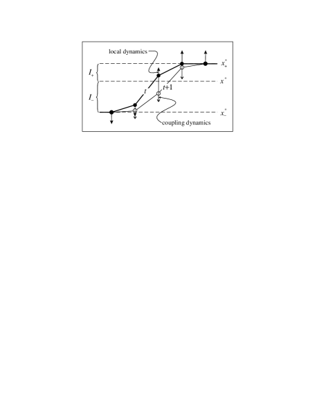
FIG. 1.: The dynamics of a front for a one-way CML results from the competition between local dynamics and coupling. The schematic contributions from the local dynamics (arrows with filled arrow-head) and coupling (arrows with empty arrow-head) are depicted for all front sites at time $t$ (filled circles). A sufficiently large coupling causes a site located within the basin $I_{+}$ (filled circle at the centre of front) to switch to the basin $I_{-}$, and move rapidly towards $x_{-}^{*}$. As a consequence, the centre of mass of the front will move to the right, resulting in propagation.

A similar argument can be applied in the diffusive case. Now however the coupling is symmetric, and a bias to either of the stable points will have to be introduced via an asymmetry in the local map. For instance, increasing the size of the basin of attraction of $x_{-}^{*}$, will result in propagation from left to right for an increasing front.

In previous works we have shown that the dynamics of a finite-size interface in a class of piece-wise linear one-way CMLs can be reduced to a single one-dimensional map [9, 10]. The finiteness of the front depended on the existence of degenerate superstable fixed points of the local map, that caused nearby orbits to collapse unto the stable states in a single iteration. In this paper we remove such degeneracy, and consider smooth local maps and infinitely extended fronts (the case of a discontinuous local map was treated in [11]). We shall provide evidence that every front evolves towards a unique asymptotic regime, characterized by a constant velocity as well as an invariant shape. Under these assumptions, we then show how the front behaves at the boundary of the regions of parametric stability (here the continuity of the local map is essential), and how the reduction to one-dimensional dynamics can be achieved.

This paper is organised as follows. In section II we describe the behaviour of travelling fronts in the continuum limit, when the density of interfacial sites is large. We obtain an ODE describing the shape of the travelling front, and with it we find new classes of fronts. In section III we consider the asymptotic shape of the front, and we provide extensive evidence that such a shape is fixed and is described by a continuous function. This result allows us to derive a procedure for the reduction of the infinite-dimensional interface dynamics to a one-dimensional problem described by the auxiliary map. In section IV we show that the auxiliary map is a circle map and we relate its rotation number to the velocity of the front, from which the mode-locking of the velocity with respect to the system parameters follows. Finally, we explain in terms of reduced dynamics the vanishing effect of mode-locking when the continuum limit is approached.

II The continuum limit

In this section we consider fronts with large widths, for which the relative density of sites is large, and the continuum approximation becomes appropriate. To achieve a front with such features, the attraction towards $x_{\pm}^{*}$ and the repulsion of $x^{*}$ must be small. Because $f$ is continuous and monotonic, then $f$ is necessarily close to the identity, i.e.

$$\delta_{f}=\sup_{x^{*}_{-}<x<x^{*}_{+}}\,|f(x)-x|\,\ll\,1.$$

Choosing functions $f$ such that $\delta_{f}\rightarrow 0$ is referred to as the continuum limit.

Inserting equation (5) into the equations of motion (1) and (2) we find that

$$\begin{array}[]{lrcl}\hbox{\rm a)}&h(z-v)&=&(1-\varepsilon)f(h(z))+\varepsilon f(h(z-1)),\\[12.91663pt] \hbox{\rm b)}&h(z-v)&=&(1-\varepsilon)f(h(z))\\[4.30554pt] &&&+\displaystyle{\varepsilon\over 2}\left(f(h(z-1))+f(h(z+1))\right),\end{array}$$ (6)

for the one-way and diffusive CML, respectively, where $z=i-vt$. A function $h$ satisfying the functional equation (6) represents the fixed shape of a front travelling at the velocity $v$.

To solve equation (6) in the continuum limit, we assume $f$ and $h$ to be twice differentiable, and consider the Taylor series of $h$ in $z$, up to second order. The Taylor expansion becomes accurate as the width increases, since in this case the variation of $h$ over adjacent lattice sites tends to zero. We obtain

$$\begin{array}[]{rl}h(z)-f(h(z))&+A\,h^{\prime}(z)-\displaystyle\left({{\displaystyle\varepsilon\,f^{\prime\prime}(h(z))}\over\displaystyle 2}\right){h^{\prime}(z)}^{2}\\[8.61108pt] &+\displaystyle\left({\displaystyle v^{2}-\varepsilon\,f^{\prime}(h(z))\over\displaystyle 2}\right)h^{\prime\prime}(z)\,=\,0,\end{array}$$ (7)

where $A=\left(\varepsilon\,f^{\prime}(h(z))-v\right)$ and $A=-v$, for the one-way and diffusive CML, respectively. In the continuum limit we can further simplify equation (7) by considering $f^{\prime}(x)=1$ and $f^{\prime\prime}(x)=0$, to obtain

$$\begin{array}[]{ll}\hbox{\rm a)}&h(z)-f(h(z))+\displaystyle\left({\displaystyle\varepsilon(\varepsilon-1)\over\displaystyle 2}\right)h^{\prime\prime}(z)=0,\\[17.22217pt] \hbox{\rm b)}&h(z)-f(h(z))-v\,h^{\prime}(z)+\displaystyle\left({\displaystyle v^{2}-\varepsilon\over\displaystyle 2}\right)h^{\prime\prime}(z)=0,\end{array}$$ (8)

for the one-way and diffusive CML, respectively, where we set $v=\varepsilon$ in the one-way case since in the continuum limit $f(x)\rightarrow x$ and thus the rate of information exchange (i.e. the velocity) is equal to $\varepsilon$. For the diffusive case the velocity is not equal to $\varepsilon$, since the total information exchange comes from the competition between the left and right neighbours. Nevertheless, as we shall see, it is possible to give an analytical approximation to the velocity for the case of an asymmetric cubic local map.

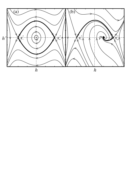
FIG. 2.: Phase space $h^{\prime}(t)$ vs. $h(t)$ of the ODEs (8) corresponding to the travelling front solution in the continuum limit. (a) A one-way CML corresponds to Hamiltonian motions. (b) A diffusive CML corresponds to dissipative motions. Note that in (b) an heteroclinic connection between unstable points can still exist in presence of friction.

Equations (8) are similar to those obtained in [17], where the travelling front in a lattice of coupled ODEs, is reduced to a single equation. The ODEs (8) describe the motion of a particle of mass $m=(v^{2}-\varepsilon)/2$, subject to the potential $V(x)=\int{(f(x)-x)\,dx}$, with maxima located at the stable fixed points of the local map (Figure 2).

In the one-way case, the system is conservative. For numerical experiments, we choose a symmetric local map $f$ with fixed point $x_{\pm}^{*}=\pm 1$ and $x^{*}=0$. The resulting potential is also symmetric. There exist two heteroclinic connections, joining $x_{-}^{*}$ to $x_{+}^{*}$, and $x_{+}^{*}$ to $x_{-}^{*}$, respectively (the thick lines in Figure 2(a)). They correspond, respectively, to an increasing and a decreasing symmetric travelling front for the CML.

In the diffusive case, the differential equation has the dissipative term $-v\,h^{\prime}(z)$. For the local map, we choose $0<x^{*}=p<1$, which introduces an asymmetry in the system, and the maxima of the potential are now unequal: $V(x_{-}^{*})>V(x_{+}^{*})$. Imposing a heteroclinic connection from $x_{-}^{*}$ and $x_{+}^{*}$, constrains the velocity $v$ of the front (see below). For larger velocities, the separatrix emanating from $x_{-}^{*}$ approaches $p$, while for smaller $v$ it escapes to infinity. Since the presence of friction breaks the time-reversal symmetry, only one heteroclinic connection is possible, and the separatrix emanating from $x_{+}^{*}$ always approaches $p$ (the thick lines in Figure 2(b)).

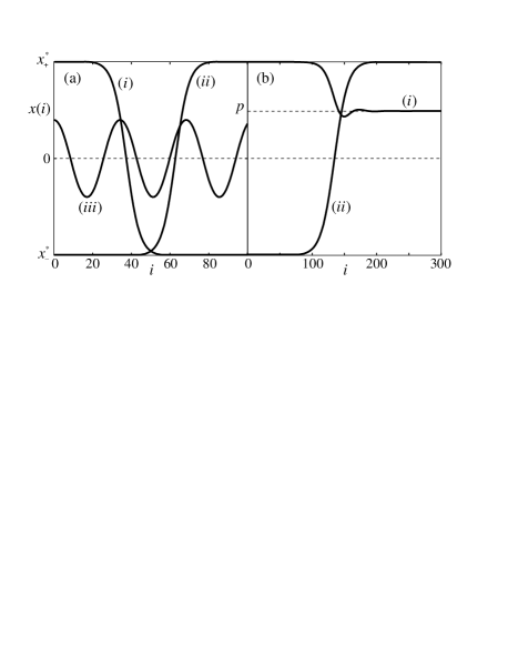
FIG. 3.: Travelling front solutions in the continuum limit approach. (a) Heteroclinic ($(i)$ and $(ii)$), and oscillatory $(iii)$ solutions in a one-way CML. (b) Damped heteroclinic solutions: $(i)$ connects the stable fixed point $x_{+}^{*}$ to the unstable fixed point $x^{*}=p$; $(ii)$ connects the two stable points.

The continuum approximation can be used to construct new kinds of travelling fronts. For example, the librating orbits in Figure 2(a) (one-way case), correspond to spatially-periodic travelling fronts that never touch the stable points (see Figure 3(a) $(iii)$). Such spatially-periodic orbits do not exist in the diffusive case. Nevertheless, it is possible to construct the travelling front departing from $x_{+}^{*}$ that dissipates down to $p$. This new solution has a damped oscillatory profile (see Figure 3(b) $(i)$), and it is unstable, because the fixed point at $p$ is unstable (for the CML).

In the remainder of this section, we briefly examine the case of a cubic local map, providing the dominant behaviour of a general bistable local map in the continuum limit. We use the one-parameter families of cubics

$$\begin{array}[]{ll}\hbox{\rm a)}&f(x)={\displaystyle x\over\displaystyle 2}(3-\nu-(1-\nu)\,x^{2})\,,\\[17.22217pt] \hbox{\rm b)}&f(x)=(1-\nu)\,(p\,x^{2}-x^{3}-p)+(2-\nu)\,x.\end{array}$$ (9)

for the one-way and diffusive CML, respectively. Again, $x_{\pm}^{*}=\pm 1$ for both cases, while $x^{*}=0$ in the one-way case and $x^{*}=p$ in the diffusive case, where $0<p<1$ controls the asymmetry. The continuum limit is attained by letting the parameter $\nu$ approach 1 from below. Substituting the cubic local maps (9) in the differential equations (8), one finds expressions for the heteroclinic connections corresponding to the travelling front solutions:

$$\begin{array}[]{ll}\hbox{\rm a)}&h(z)=\tanh\left(\sqrt{\displaystyle 1-\nu\over\displaystyle 2\varepsilon(1-\varepsilon)}\,z\right),\\[17.22217pt] \hbox{\rm b)}&h(z)=\tanh\left({\displaystyle(1-\nu)p\over\displaystyle v}\,z\right),\end{array}$$ (10)

where

$$\begin{array}[]{lll}\hbox{\rm a)}&v=\varepsilon&\quad\displaystyle\sigma^{2}={2\pi^{2}\over 3}{\varepsilon(1-\varepsilon)\over 1-\nu}\\[17.22217pt] \hbox{\rm b)}&v=p\sqrt{\varepsilon(1-\nu)}&\quad\displaystyle\sigma^{2}={\pi^{2}\over 3}{\varepsilon\over 1-\nu}.\end{array}$$ (11)

for the one-way and diffusive CML, respectively. In the diffusive case, the expression for the velocity is derived from imposing an heteroclinic connection, while the scaling of the width $\sigma^{2}$ is found from the solutions (10). Note that for both models the functional dependence of the width on the parameter $\nu$ is the same, and it describes the rate at which the front broadens as the continuum limit is approached. Moreover, from (10) and (11) we have that in the diffusive case $h$ is independent of $p$.

While in the continuum limit the front is described by a continuous function $h$ (cf. equations (10)), there is no a-priori reason why such a function should continue to exist away from the limit, due to the discrete nature of the system. We shall nonetheless give evidence that the dynamics of a front far from the continuous limit remains one-dimensional.

III Reduced dynamics of the travelling front

In this section we provide evidence that every front has a fixed profile, which can be characterized by an invariant function $h$. Such a function will then be used to construct a one-dimensional mapping describing the front evolution —the auxiliary map.

If the velocity $v$ of the front is irrational, then the collection of points $i-vt$, with $i$ and $t$ integers, form a set dense on the real line. Numerical experiments consistently suggest that in the case of a front, the closure of the set of points $(i-vt,\,x_{t}(i))\in{{R}}^{2}$ forms the graph of a continuous and monotonic function: $h:{{Z}}\mapsto[x_{-}^{*},\,x_{+}^{*}]$, which is a solution to the functional equation (6).

The results for both CML models are summarised in Figure 4, where we have superposed all translates of the discrete fronts, after eliminating transient behaviour. This procedure requires computing $v$ numerically, which was done using some $10^{7}$–$10^{8}$ iterations of the CML. (In principle, a numerical solution to (6) can be found using various iterative functional schemes. However, all the schemes considered were plagued by slow convergence and are not discussed here.)

FIG. 4.: The travelling front shape is reconstructed by superimposing snapshots of the discrete interface in a co-moving reference frame. (a) One-way coupling: $f(x)=\tanh(x/0.2)$, $\varepsilon=0.398011$, $v(\varepsilon)\simeq 0.2856031\simeq 2/7$. (b) Diffusive coupling: $f$ is the second iterate of the logistic map, with $\varepsilon=0.2$ and $v(\varepsilon)\simeq 0.0097915$; (c) Diffusive coupling: $f$ as in (b), with $\varepsilon=0.6$ and $v(\varepsilon)\simeq 0.1118273$.

In the case in which $v=p/q$ is rational, the function $h$ is specified only at a set of $q$ equally spaced points. It turns out, however, that the definition of $h$ becomes unequivocal in a prominent parametric regime, corresponding to the boundary of the so-called mode-locking region or tongue. The latter is defined as the collection of parameters $(\varepsilon,\nu)$ corresponding to a given rational velocity, where $\nu$ (not necessarily one-dimensional) parametrizes the family of local maps —for the one-way CML we typically use $f(x)=\tanh(x/\nu)$.

We defer the discussion of the origin of such regions to the next section. Here we consider a sequence of parameters $(\varepsilon_{n},\nu_{n})\rightarrow(\varepsilon_{*},\nu_{*})$, converging from the outside towards a boundary point $(\varepsilon_{*},\nu_{*})$ of the tongue (see Figure 5). Independently from the path chosen to approach the boundary point, the front $h$ appears to approach a unique limiting shape. The limiting shape is a step function with $q$ steps (where $v=p/q$) for every unit length —the horizontal length of each step is $1/q$ since there are $q$ equidistant points in every horizontal interval of unit length for a $v=p/q$ orbit. In the limit, the front dynamics becomes periodic, with periodic points corresponding to the midpoint of each step. This observation suggests that choosing step fronts with the periodic points at their midpoints ensures continuity of the front shapes at the resonance tongue boundaries.

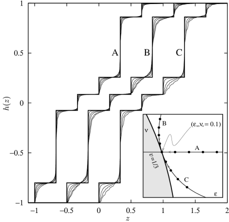
FIG. 5.: Approximating travelling front for a rational velocity. The parametric point located at the edge of a tongue (small box), is approached both transversally (path $A$) and tangentially (paths $B$ and $C$). The tongue corresponds to a travelling front with velocity $v(\varepsilon)=1/3$, which is periodic with period 3. In all cases the front shape approaches the same step function, with 3 steps per unit length in $z$. Note that the fronts have been shifted for clarity. Here the local map is $f(x)=\tanh(x/\nu)$, and the parameters at the boundary of the mode-locking region are $(\varepsilon_{*}=0.3983,\nu_{*}=0.1)$.

In the next section, we shall explain this phenomenon in terms of the dynamics of a one-dimensional map —the auxiliary map $\Phi$— which we now define. The idea is to describe the evolution of any site in the front by means of a single site, the central site $\bar{x}_{t}(0)$, defined as the site which is closest to the unstable point $x^{*}$. The position of the central site moves along the lattice with an average velocity $v(\varepsilon)$, since it follows the centre of the interface. Following [9, 10], we define the map $\Phi$ as

$$\bar{x}_{t+1}(0)=\Phi(\bar{x}_{t}(0)).$$ (12)

If the velocity is irrational, the domain of definition of the map is a set of points dense in an interval (see next section), and the possibility exists of extending $\Phi$ continuously to the interval. In Figure 6(a) and (b), we plot the graph of $\Phi$ for a one-way and a diffusive CML, respectively. The auxiliary map corresponds to the square region depicted with thick lines, while the other regions represent delay Poincaré maps of some neighbouring sites. Indeed for each neighbour $j$ of the central site, there is a corresponding auxiliary circle map $\Phi_{j}$, such that $\bar{x}_{t+1}(j)=\Phi_{j}(\bar{x}_{t}(j))$, with $\Phi=\Phi_{0}$ (see below).

FIG. 6.: Auxiliary maps $\Phi$ for the central site of the interface defined in the square region depicted by the thick lines. (a) one-way CML: local map $f(x)=\tanh(x/0.2)$ with $\varepsilon=0.4$, $v=0.28973453$. (b) Diffusive: same parameters as in Figure 4(c). The delay Poincaré section $\Phi(x)$ corresponds to the central rectangular region of each plot (region 1) in Figure (a). Each rectangular region corresponds to the return map for a particular combination of sites. For instance, the region 2) in Figure (a) corresponds to $\bar{x}_{t+1}(1)$ vs. $\bar{x}_{t}(1)$.

If the velocity is rational, equation (12) defines $\Phi$ only at a finite set of points, and to extend the domain of definition, one must make use of equation (12) on suitable transients. We have verified numerically that when a front is perturbed, the perturbation relaxes quickly onto a one-dimensional manifold, along which the original front is approached. The process of randomly disturbing the front amounts to a random walk path reconstruction of the one-dimensional manifold. Such one-dimensional transients were found to be independent of the detail of the perturbation, giving a unequivocal definition of the auxiliary map also in the rational case. This is illustrated in Figure 7. Crucially, this construction yields a map that changes continuously within the tongue, matching the the behaviour at the boundary of the tongue. Thus we conjecture that the auxiliary map $\Phi$ depends continuously on the coupling parameter $\varepsilon$. In the next section we shall explore some consequences of the continuity.

FIG. 7.: Typical reconstruction of the auxiliary map $\Phi$ inside a mode-locking tongue. The large stars locate the original periodic orbit well inside a tongue (in this example $v=1/5$). A small random perturbation is periodically applied to the central site of the front. The state of each perturbed front is depicted by circles. After few transient iterations (2 or 3), the perturbed front relaxes onto the one-dimensional manifold represented by the thick line. This technique is applied repeatedly until the whole one-dimensional manifold is filled in.

We finally relate the dynamics of the entire front to that of the central site, governed by $\Phi(x)$. Let $\bar{x}_{t}(j)$ denote the $j$-th neighbouring site of the central site $\bar{x}_{t}(0)$, where $j$ is positive (negative) for the right (left) neighbours. The dynamics of $\bar{x}_{t}(j)$ can be deduced from that of $\bar{x}_{t}(0)$ and the knowledge of $h$, as follows

$$\bar{x}_{t}(j)=h\circ\tau_{j}\circ h^{-1}(\bar{x}_{t}(0))$$ (13)

where $\tau_{j}$ is the translation by $j$ on ${{R}}$. Since $\Phi_{j}(x)$ maps $\bar{x}_{t}(j)$ to $\bar{x}_{t+1}(j)$, the pair $\left(\bar{x}_{t}(j),\,\bar{x}_{t+1}(j)\right)$ belongs to the graph of $\Phi_{j}$. By applying the operator $h\circ\tau_{j}\circ h^{-1}$ to the function $\Phi(\bar{x}_{t}(0))$ we obtain:

$$\begin{array}[]{rcl}h\circ\tau_{j}\circ h^{-1}\Phi(\bar{x}_{t}(0))&=&h\circ\tau_{j}\circ h^{-1}(\bar{x}_{t+1}(0))\\[8.61108pt] &=&\bar{x}_{t+1}(j)\,=\,\Phi_{j}\left(\bar{x}_{t}(j)\right),\end{array}$$

where we used equation (13) which relates neighbouring sites. Thus $h\circ\tau_{j}\circ h^{-1}$ provides a conjugacy between $\Phi$ and $\Phi_{j}$ and enables us to reconstruct the whole interfacial dynamics from the behaviour of the central site.

IV Mode-locking of the propagation velocity

In this section we show that the auxiliary map $\Phi$ is a circle homeomorphism (see Figure 8). The mode-locking of the front velocity will then follow from the mode-locking of the rotation number of $\Phi$. Furthermore, the conjectured continuous dependence of $\Phi$ on $\varepsilon$ implies a continuous dependence of the rotation number on $\varepsilon$, and in particular, $\Phi$ takes all rotation numbers between any two realised values. For instance, the front velocity in a one-way CML takes the values $0$ and $1$ for $\varepsilon=0$ and $1$, respectively, and thus as the coupling parameter varies, all velocities $v\in[0,1]$ are realised. For a diffusive CML only an interval $[0,v_{max}]$ is attained since the maximum velocity $v_{max}=v(\varepsilon=1)$ does not reach 1 because of the competition between the attractors.

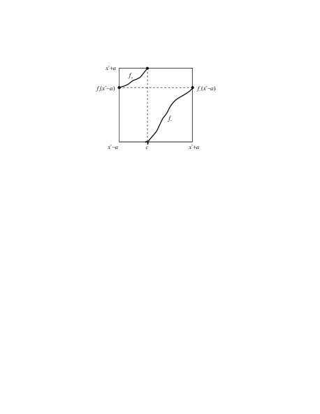
FIG. 8.: The auxiliary map $\Phi$, accounting for the dynamics of the site closest to the unstable point $x^{*}$, is a circle map on $[x^{*}-a,x^{*}+a]$, with two increasing branches $f_{+}$ and $f_{-}$.

Let us consider a continuous and increasing travelling front $h(i-vt+i_{0})$ with positive irrational velocity $0<v<1$. The largest possible separation between $\bar{x}_{t}(0)$ and $x^{*}$ corresponds to the position of $h$ for which two consecutive points on the lattice are equally spaced from the unstable point $x^{*}$. Suppose that the front shape $h$ is positioned such that for site $i$, we have $h(i)=x^{*}$. We choose $\alpha$ such that

$$h(i-\alpha)=x^{*}-a\quad{\rm and}\quad h(i+1-\alpha)=x^{*}+a$$ (14)

where $0\leq a\leq\min(|x_{+}^{*}-x^{*}|,|x_{-}^{*}-x^{*}|)$. By adding the two equations in (14) one obtains an equation for $\alpha$, and $a$ can then be evaluated. If the front is at a position where it satisfies the equations (14) for some $i$, then the $i$-th and $(i+1)$-th sites are equally spaced from $x^{*}$, and the dynamics of the site closest to $x^{*}$ is contained in the interval $[x^{*}-a,x^{*}+a]$. Any shift of the front will cause either one of the two sites to be closer to $x^{*}$ than originally.

We now follow the dynamics of $\bar{x}_{t}(0)$ in $[x^{*}-a,x^{*}+a]$. Suppose that at time $\tau$ the $i$-th site is the closest to $x^{*}$ so $\bar{x}_{\tau}(0)=x_{\tau}(i)$. We want to know which site will be closest to $x^{*}$ at time $\tau+1$. Since we are considering the case $v>0$ there are two possibilities: a) the $i$-th site again ($\bar{x}_{\tau+1}(0)=x_{\tau+1}(i)$) or b) the $(i+1)$-th site ($\bar{x}_{\tau+1}(0)=x_{\tau+1}(i+1)$). Redefining $h_{t}(i)=h(i-vt+i_{0})$, we find two cases

$$h_{\tau+1}^{-1}(\bar{x}_{\tau+1}(0))=\left\{\begin{array}[]{ll}h_{\tau}^{-1}(\bar{x}_{\tau}(0))&\quad\mbox{(a)}\\[8.61108pt] h_{\tau}^{-1}(\bar{x}_{\tau}(0))+1&\quad\mbox{(b)}\end{array}\right..$$ (15)

But, by definition, $h_{\tau+1}(x)=h_{\tau}(x-v)$, so from equation (15) one obtains

$$\bar{x}_{\tau+1}(0)=\left\{\begin{array}[]{ll}f_{-}(\bar{x}_{\tau}(0))&\quad\mbox{(a)}\\[8.61108pt] f_{+}(\bar{x}_{\tau}(0))&\quad\mbox{(b)}\end{array}\right.$$ (16)

where

$$\begin{array}[]{rcl}f_{-}(x)&=&h_{\tau}\left(h_{\tau}^{-1}(x)-v\right)\\[8.61108pt] f_{+}(x)&=&h_{\tau}\left(h_{\tau}^{-1}(x)-v+1\right).\end{array}$$ (17)

The functions $f_{-}$ and $f_{+}$ inherit some of the properties of $h$. In particular, $f_{-}$ and $f_{+}$ are continuous and increasing. In the the interval $[x^{*}-a,x^{*}+a]$ we have that $f_{-}(x)<f_{+}(x)$, because $h$ is increasing, so we just evaluate at the following points:

$$\begin{array}[]{rcl}f_{-}(x^{*}+a)&=&h_{\tau}(h_{\tau}^{-1}(x^{*}+a)-v)\\[4.30554pt] &=&h_{\tau}(i+1-\alpha-v)\\[12.91663pt] f_{+}(x^{*}-a)&=&h_{\tau}(h_{\tau}^{-1}(x^{*}-a)-v+1)\\[4.30554pt] &=&h_{\tau}(i-\alpha-v+1)\end{array}$$

where we have made use of equations (14). Thus we have the periodicity condition

$$f_{-}(x^{*}+a)=f_{+}(x^{*}-a).$$ (18)

Next we find when $f_{-}$ and $f_{+}$ reach the extrema of the interval $[x^{*}-a,x^{*}+a]$. To this end we determine $c_{\pm}$ such that $f_{\pm}(c_{\pm})=x^{*}\pm a$. So we solve

$$\begin{array}[]{rl}&\left\{\begin{array}[]{rcccl}f_{-}(c_{-})&=&h_{\tau}(h_{\tau}^{-1}(c_{-})-v)&=&x^{*}-a\\[8.61108pt] f_{+}(c_{+})&=&h_{\tau}(h_{\tau}^{-1}(c_{+})-v+1)&=&x^{*}+a\end{array}\right.\\[21.52771pt] \Rightarrow&\left\{\begin{array}[]{rcccl}h_{\tau}^{-1}(c_{-})-v&=&h_{\tau}^{-1}(x^{*}-a)&=&i-\alpha\\[8.61108pt] h_{\tau}^{-1}(c_{+})-v+1&=&h_{\tau}^{-1}(x^{*}+a)&=&i+1-\alpha\end{array}\right.\\[25.83325pt] \end{array}$$

whence $h_{\tau}^{-1}(c_{-})=h_{\tau}^{-1}(c_{+})$, and since $h$ is monotonic, we have that $c_{-}=c_{+}=c.$

Therefore, the map $\Phi$ giving the dynamics of the central site (12) is given by

$$\Phi(x)=\left\{\begin{array}[]{lrcccl}f_{+}(x)&\mbox{~{}~{}if~{}~{}}x^{*}-a&\leq&x&\leq&c\\[8.61108pt] f_{-}(x)&\mbox{~{}~{}if~{}~{}}x^{*}+a&\geq&x&>&c.\end{array}\right.$$ (19)

From the above properties of $f_{-}$ and $f_{+}$, it follows that the auxiliary map $\Phi$ is a homeomorphism of the circle (see Figure 8).

A natural binary symbolic dynamics for $\Phi$ is introduced by assigning the symbols ‘0’ and ‘1’ whenever the branch $f_{-}$ or $f_{+}$, respectively, is used in (15). These symbols corresponds to the central site $x(i)$ remaining unchanged, or being replaced by the new site $x(i+1)$, respectively.

FIG. 9.: Onset of intermittent regime in the auxiliary map, corresponding to the development of a step-like travelling front. For the parameter values and the front shape please refer to Figure 4(c). The intermittency is the precursor of a pair of period-7 orbits.

Every time a ‘1’ is encountered, the front advances by roughly one site. So the density of ‘1’s in the sequence gives an approximation to the velocity, which becomes exact in the limit $t\rightarrow\infty$. In terms of the circle map, the proportion of ‘1’s in the sequence corresponds to its rotation number $\rho$:

$$\rho(\varepsilon)=v(\varepsilon)=\lim_{t\rightarrow\infty}{{\displaystyle 1\over\displaystyle t}\sum_{i=1}^{t}{s_{i}}},$$ (20)

where $s_{i}$ is the $i$-th term in the symbolic sequence. We have stressed the $\varepsilon$-dependence of $\rho$, since for a fixed local map, $\Phi$ depends on $\varepsilon$, and so does its rotation number. Because all sites $\bar{x}(j)$ belong to the same front, the site interchanges all occur at the same time, and therefore the rotation number of any $\Phi_{i}$ is the same as the one for $\Phi$.

The representation of the motion of a front as a circle map implies the likelihood of mode-locking for rational velocities, corresponding to Arnold tongues in parameter space, and it affords a simple explanation of the various dynamical phenomena described in the previous sections.

The appearance of a $q$-period tongue as $\varepsilon$ is varied thorough some critical value $\varepsilon_{*}$, corresponds to a fold bifurcation of $\Phi^{q}$. Generically, a pair of period-$q$ orbits is created at $\varepsilon=\varepsilon_{*}$. Thus the orbits of $\Phi$ will undergo intermittency in the region of the period-$q$ orbit for $\varepsilon_{n}$ close to $\varepsilon_{*}$. The intermittency will manifest itself in the graph of $\Phi$ as shown by the darkly shaded areas of the orbit web in Figure 9.

Moreover, the periodic orbit will form towards the centre of the dark bands and the corresponding front shape will “flatten” at the heights taken by the periodic points because of the time spent in their neighbourhood by the orbits of $\Phi$ for $\varepsilon_{n}\approx\varepsilon_{*}$. It then follows that the approximating fronts will form steps for the periodic front with the periodic points close to their centre points, and independently from the parametric path chosen to approach the boundary point (see Figure 5).

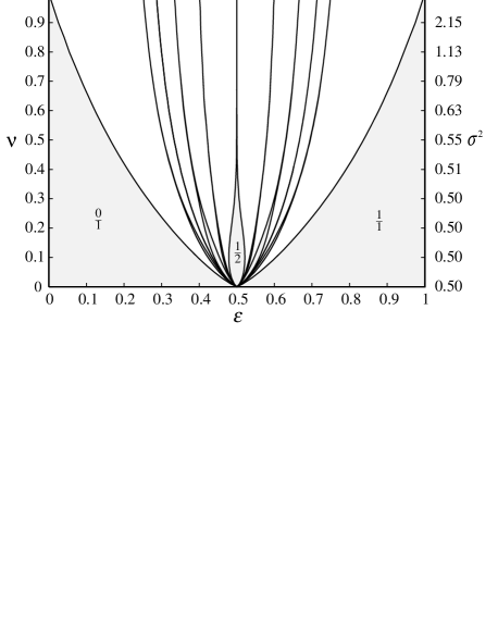
FIG. 10.: Principal Arnold’s tongues of the travelling front velocity in the one-way CML with the hyperbolic tangent local map $f(x)=\tanh(x/\nu)$ in the $(\varepsilon,\nu)\in[0,1]^{2}$ parameter space. The right hand side scale gives the width $\sigma^{2}$ of the corresponding travelling front for fixed $\varepsilon=1/2$.

In Figure 10 we plot the main mode-locking regions in parameter space (Arnold tongues), corresponding to $v=p/q$ with small $q$. Here the local map is given by $f(x)=\tanh(x/\nu)$, while the parameters vary within the unit square: $(\varepsilon,\nu)\in[0,1]^{2}$. We believe that mode-locking is a common phenomenon in front propagation in CMLs, because the nonlinearity of the local map induces nonlinearity in the auxiliary map [9, 10], and mode-locking is generic for such maps. However, this phenomenon often takes place on very small parametric scales, since the width of the tongues decreases sharply with increasing $\nu$ (Figure 10). This explains why this phenomenon has not been widely reported (with the notable exception of the large $v=0$ region, corresponding to the well-known propagation failure in the anti-continuum limit [18]).

FIG. 11.: Auxiliary maps $\Phi_{i}(x)$ for the reduced dynamics of the travelling front near the continuum limit. The CML was taken to be one-way with local map $f(x)=\tanh(x/\nu)$, $\nu=100/101$ and coupling strength $\varepsilon=0.45$.

In the continuum limit (see Figure 10), the stability of the attractors $x_{\pm}^{*}$ becomes weaker, causing the front to broaden. In Figure 11 we plotted the auxiliary maps $\Phi_{i}$ corresponding to $\nu=100/101\simeq 1$ for the one-way CML with local map $f(x)=\tanh(x/\nu)$. This figure should be compared with Figure 6, corresponding to a narrower front. The domain of each $\Phi_{i}$ is now smaller, since the interval $I=[x_{-}^{*},x_{+}^{*}]$ has to be shared between a larger number of sites. As a consequence, the nonlinearity of each $\Phi$ is reduced (note that the auxiliary maps in Figure 11 are almost linear) and with it the size of the tongues. Thus, the larger the width $\sigma^{2}$ of the travelling front, the thinner the mode-locking tongue (see right hand side scale in Figure 10).

REFERENCES

- [1] K. Kaneko. Period-doubling of kink-antikink patterns, quasiperiodicity in anti-ferro-like structures and spatial intermittency in coupled logistic lattice. Prog. Theor. Phys. 72, 480 (1984); I. Waller and K. Kapral. Spatial and temporal structure in systems of coupled nonlinear oscillators. Phys. Rev. A 30, 2047 (1984); J. Crutchfield. Space-time dynamics in video feedback. Physica D 10, 229 (1984).
- [2] C. Beck. Chaotic cascade model for turbulent velocity distribution. Phys. Rev. E 49, 3641 (1994); K. Kaneko. Spatiotemporal chaos in one- and two-dimensional coupled map lattices. Physica D 37, 60 (1989).
- [3] T. Yanagita and K. Kaneko. Coupled map lattice model for convection. Phys. Lett. A 175, 415 (1993).
- [4] F.H. Willeboordse and K. Kaneko. Pattern dynamics of a coupled map lattice for open flow. Physica D, 101 (1995).
- [5] R. Kapral, R. Livi, G.-L. Oppo and A. Politi. Dynamics of complex interfaces. Phys. Rev. E 49, 2009 (1994).
- [6] M.P. Hassell, O. Miramontes, P. Rohani and R.M. May. Appropriate formulations for dispersal in spatially structured models. J. Anim. Ecology 64, 662 (1995); R.V. Solé and J. Bascompte. Measuring chaos from spatial information. J. theo. Biol. 175, 139 (1995);
- [7] K. Kaneko. Global travelling wave triggered by local phase slips. Phys. Rev. Lett. 69, 905 (1992); K. Kaneko. Chaotic travelling waves in a coupled map lattice. Physica D 68, 299 (1993).
- [8] R. Carretero-González. Front propagation and mode-locking in coupled map lattices. PhD thesis, Queen Mary and Westfield College, University of London (1997). http://www.ucl.ac.uk/ucesrca/abstracts.html.
- [9] R. Carretero-González, D.K. Arrowsmith and F. Vivaldi. Mode-locking in coupled map lattices. Physica D 103, 381 (1997).
- [10] R. Carretero-González, Low dimensional travelling interfaces in coupled map lattices. Int. J. Bifurcation and Chaos 7, 2745 (1997).
- [11] R. Coutinho and B. Fernandez, Fronts and interfaces in bistable extended mappings. Nonlinearity 11, 1407 (1988).
- [12] L.M. Floria and J. Mazo, Dissipative dynamics of the Frenkel-Kontorova model. Advances in Physics 45, 505 (1996).
- [13] M. Basler, W. Krech and K.Y. Platov. Theory of phase-locking in generalized hybrid Josephson-junction arrays. Phys. Rev. B 55, 1114 (1997).
- [14] J. Kosek, I. Schreiber and M. Marek. Phase mappings from diffusion-coupled excitable chemical media. Phil. Trans. R. Soc. Lond. A 347, 643 (1994).
- [15] P.C. Bressloff, S. Coombes and B. deSouza. Dynamics of a ring of pulse-coupled oscillators: Group theoretic approach. Phys. Rev. Lett. 79, 2791 (1997); R. Kuske and T. Erneux. Bifurcation to localized oscillations. Euro. J. Appl. Math. 8, 389 (1997).
- [16] P.M. Gade and R.E. Amritkar. Spatially periodic orbits in coupled map lattices. Phys. Rev. E 47, 143 (1993); Q. Zhilin, H. Gang, M. Benkun and T. Gang. Spatiotemporally periodic patterns in symmetrically coupled map lattices. Phys. Rev. E 50, 163 (1994).
- [17] S.N. Chow and J. Mallet-Paret. Pattern formation and spatial chaos in lattice dynamical systems. IEEE Transactions on circuits and systems I 42, 746 (1995); S.N. Chow, J. Mallet-Paret and E.V. Vleck. Dynamics of lattice differential equations. Int. J. Bifurcation and Chaos 6, 1605 (1996).
- [18] S. Aubry and G. Abramovici. Chaotic trajectories in the standard map. The concept of anti-integrability. Physica D 43, 199 (1990); R.S. MacKay and J.-A. Sepulchre. Multistability in networks of weakly coupled bistable units. Physica D 82, 243 (1995).