Spectral properties of Dissipative Chaotic Quantum Maps

I examine spectral properties of a dissipative chaotic quantum map with the help of a recently discovered semiclassical trace formula. I show that in the presence of a small amount of dissipation the traces of any finite power of the propagator of the reduced density matrix, and traces of its classical counterpart, the Frobenius–Perron operator, are identical in the limit of $\hbar\to 0$. Numerically I find that even for finite $\hbar$ the agreement can be very good. This holds in particular if the classical phase space contains a strange attractor, as long as one stays clear of bifurcations. Traces of the quantum propagator for iterations of the map agree well with the corresponding traces of the Frobenius–Perron operator if the classical dynamics is dominated by a strong point attractor.

I Introduction

The interplay between chaos, quantum mechanics and dissipation is rather complex and the subject of strong current research activities [1, 2, 3, 4, 5, 6]. The definition of chaos in classical mechanics via exponentially fast spreading trajectories can not be applied to quantum mechanical systems, since the notion of a trajectory does not exist in quantum mechanics. On a quantum mechanical level chaos manifests itself in the statistical properties of the eigenenergies and eigenfunctions. In the case of Hamiltonian systems the eigenenergies and eigenfunctions obey the universal statistics of large random hermitian matrices restricted only by general symmetry requirements like invariance under time and spin reversal [7, 8]. While no rigorous proof of this conjecture is known yet, overwhelming numerical and experimental evidence has been accumulated [9, 10, 11].
Dissipation has at least two very important effects. The classical dynamics is altered profoundly. It is no longer restricted to a shell of constant energy in phase space, but phase space volume shrinks if no external source compensates for the energy dissipated. In a chaotic system with external driving dissipation typically leads to a strange attractor in phase space, i.e. a multi-fractal structure that is invariant under the dynamics and which has a dimension strictly smaller than the dimension of the phase space. The second effect is of quantum mechanical nature and more subtle: Dissipation destroys very efficiently the quantum mechanical phase information. This typically happens on time scales much shorter than classical ones and even with very tiny amounts of dissipation [12, 13, 14]. Therefore the system behaves more classically, and one might expect to find classical manifestations of chaos again. It was indeed shown in a variety of examples that appropriate quantum mechanical counterparts of the classical phase space density (like Husimi functions or Wigner distributions) approach a smeared out version of the strange attractor [4, 15, 16]. At the same time one might ask whether spectral properties approach their classical counterparts as well. This paper shows that for certain spectral properties the answer is “YES”, even though the structure of the spectrum can be very different in both cases.

My analysis is based on a recently discovered trace formula for dissipative systems which, in the spirit of Gutzwiller’s celebrated formula [17, 18], expresses traces of the propagator of the density matrix in terms of classical periodic orbits [20]. I show in section III that to lowest order asymptotic expansion in $\hbar$ the traces agree with the traces of the classical Frobenius–Perron propagator of the phase space density [19].
In the next section I briefly review basic properties of dissipative quantum maps, semiclassical theory and the trace formula. In section IV I apply the trace formula to a dissipative kicked top and compare with numerical results for finite $\hbar$. The main results are summarized in section V.

II Dissipative Quantum Maps

A General remarks

Dissipation is introduced on a quantum mechanical level most rigorously by the so–called Hamiltonian embedding [21]. The system of interest is considered as part of a larger system including the “environment” to which energy can be dissipated. The total system is assumed to be closed so that it is adequately described by a Schrödinger equation. The degrees of freedom of the “environment” remain unobserved. The system at interest is described by a density matrix in which the environmental degrees of freedom have been traced out, usually termed the reduced density matrix $\rho(t)$.
Dissipative quantum maps are maps of the reduced density matrix from a time $t$ to a time $t+T$: $\rho(t+T)=P\rho(t)$. They are analogous to non–dissipative quantum maps, where the state vector of the system is mapped with a unitary Floquet matrix $F$, $|\psi(t+T)\rangle=F|\psi(t)\rangle$. In the dissipative case $P$ is not a unitary operator and therefore has eigenvalues inside the unit circle.
Maps, dissipative or not, are a natural description of a time evolution if an external driving of the system is periodic in time with period $T$. They give a stroboscopic picture which suffices if the evolution during one period is of no interest. Systems that are periodically driven are capable of chaos even if they have only one degree of freedom. I will restrict myself in the following to such cases.

The maps that I consider are particularly simple in the sense that the dissipation is well separated from a remaining purely unitary evolution where the latter by itself is capable of chaos. The unitary part will be described by a Floquet matrix $F$ acting on the state vector, so that the unitary evolution takes the density matrix from $\rho(t)$ to $\rho^{\prime}(t)=F\rho(t)F^{\dagger}$. After the unitary part a dissipative step follows which I will describe by a propagator $D$. It takes the density matrix from $\rho^{\prime}(t)$ to $\rho(t+T)=D\rho^{\prime}(t)$. The total map therefore reads

$$\rho(t+T)=D(F\rho(t)F^{\dagger})\equiv P\rho(t)\,.$$ (1)

Such a separation into two parts is not purely academic. A most obvious realization of (1) is given when a Hamiltonian $H(t)$ leading to the unitary evolution and the coupling to the environment can be turned on and off alternatively. This should be realizable for instance with atoms flying through a series of cavities where in each cavity either the unitary evolution or the dissipation is realized. Another example might be a billiard, in which the particle only dissipates energy when hitting the walls. But even if the dissipation cannot be turned off, the map (1) may still be a good description. For instance, if the dissipation is weak and if the entire unitary evolution takes place during a very short time, dissipation may be negligible during that time. This is the case if the entire unitary evolution is due to a periodic kicking. The dissipation can then be considered as a relaxation process between two successive kicking events. Finally, a formal reason for such a separation can be given when the generators for the unitary evolution and the dissipation commute.

These ideas might become clearer with a particular model. Let me therefore introduce as prime model system a dissipative kicked top.

B A dissipative kicked top

The dynamical variables of a top [22, 11] are the three components $J_{x,y,z}$ of an angular momentum ${\bf J}$. I will only consider dynamics (including the dissipative ones) which conserve the absolute value of ${\bf J}$, ${\bf J}^{2}=j(j+1)=const$. In the classical limit (formally attained by letting the quantum number $j$ approach infinity) the surface of the unit sphere $\lim_{j\rightarrow\infty}({\bf J}/j)^{2}=1$ becomes the phase space, such that one confronts but a single degree of freedom. Convenient phase space coordinates are

$$\mu\equiv J_{z}/J=\cos\theta=p\mbox{ and }\varphi=q,$$ (2)

where the polar and azimuthal angles $\theta$ and $\varphi$ define the orientation of the angular momentum vector with respect to the $J_{x}$, $J_{y}$ and $J_{z}$ axes. The parameter $J$ is defined as $J=j+1/2$ and allows for more convenient expressions of most semiclassical quantities. Due to the conservation of ${\bf J}^{2}$ the Hilbert space decomposes into $(2j+1)$ dimensional subspaces. The quantum dynamics is confined to one of these according to the initial conditions. The semiclassical limit is characterized by large values of the quantum number $j$ which can be integer or half integer. Since the classical phase space contains $(2j+1)$ states, Planck’s constant may be thought of as represented by $1/J$.

Consider a unitary evolution generated by the Floquet matrix

$$F={\rm e}^{-{\rm i}\frac{k}{2J}J_{z}^{2}}{\rm e}^{-{\rm i}\beta J_{y}}\,.$$ (3)

The corresponding classical motion first rotates the angular momentum by an angle $\beta$ about the $y$-axis and then subjects it to a torsion about the $z$-axis. The latter may be considered as a non–linear rotation with a rotation angle given by the $J_{z}$ component of ${\bf J}$. The dynamics is known to become strongly chaotic for sufficiently large values of $k$ and $\beta$, whereas either $k=0$ or $\beta=0$ lead to integrable motion [11]. For a physical realization of this dynamics it might be best to think of ${\bf J}$ as a Bloch vector describing the collective excitations of two–level atoms, as one is used to in quantum optics. The rotation can be brought about by a laser pulse of suitably chosen length and intensity, and the torsion by a cavity that is strongly off resonance from the atomic transition frequency [23]. The Floquet matrix (3) has also been realized in experiments with magnetic crystallites with an easy plane of magnetization [24].

Our model dissipation is defined in continuous time $\tau$ by the Markovian master equation

$$\frac{d}{d\tau}\rho(\tau)=\frac{1}{2J}([J_{-},\rho(\tau)J_{+}]+[J_{-}\rho(\tau),J_{+}])\equiv\Lambda\rho(\tau)\,,$$ (4)

where the linear operator $\Lambda$ is defined by this equation as generator of the dissipative motion. Equation (4) is well-known to describe certain superradiance experiments, where a large number of two–level atoms in a cavity of bad quality radiate collectively [25, 26]. The angular momentum operator ${\bf J}$ is then again the Bloch vector of the collective excitation and the $J_{+},J_{-}$ are raising and lowering operators, $J_{\pm}=J_{x}\pm{\rm i}J_{y}$. One easily verifies that (4) conserves the skewness in the $J_{z}$ basis ($J_{z}|m\rangle=m|m\rangle$), i.e. matrix elements $\langle m_{1}|\frac{d}{d\tau}\rho|m_{2}\rangle$ with a given skewness $J\eta=m_{1}-m_{2}$ depend only on matrix elements with the same skewness. Eq.(4) is formally solved by $\rho(\tau)=\exp(\Lambda\tau)\rho(0)$ for any initial density matrix $\rho(0)$ and this defines the dissipative propagator

$$D(\tau)=\exp(\Lambda\tau)\,.$$ (5)

Explicit forms of $D$ can be found in [25, 27, 28]. The skewness $\eta$ only enters as a parameter in $D$. The classical limit gives the simple picture of the Bloch vector creeping towards the south pole $\theta=\pi$ as an over-damped pendulum, according to the equations of motion

$$\frac{d}{d\tau}\theta=\sin\theta\mbox{, }\frac{d}{d\tau}\varphi=0\,.$$ (6)

Classically the azimuth $\varphi$ is therefore conserved. Eq.(6) also shows that $\tau$ is the time in units of the classical time scale. In the following it will be set equal to the time between two unitary steps.

The Floquet matrix (3) is usually generated by the Hamiltonian

$$H(t)=\hbar\left(\frac{k}{2JT}J_{z}^{2}+\beta J_{y}\sum_{n=-\infty}^{\infty}\delta(t-nT)\right);$$ (7)

it describes the evolution from immediately before a kick to immediately before the next kick. The generator (4) for the dissipation does not commute with $H(t)$. In order to obtain the map (1) one should replace in (7) $H_{0}=\frac{k}{2JT}J_{z}^{2}$ by $\frac{k}{2JT_{1}}J_{z}^{2}$ and switch on $H(t)$ only for a time $T_{1}<T$ during each period $T$, whereas the dissipation acts during the rest of the time $\tau=T-T_{1}$. Alternatively, when $H(t)$ and $\Lambda$ act permanently one may go to an interaction representation by $\rho(t)=\exp(-\frac{{\rm i}}{\hbar}H_{0}t)\tilde{\rho}(t)\exp(\frac{{\rm i}}{\hbar}H_{0}t)$. In the $J_{z}$ representation this leads only to phase factors in the master equation (4) which can be easily incorporated in $D$ and which vanish moreover for diagonal elements. Let us assume in the following that either has been done and use (1) with $F$ and $D$ given by (3), (4), and (5) as a starting point with $\tau$ as fixed parameter that measures the relaxation time between two unitary evolution and thus the dissipation strength.

C The trace formula

In 1970 Gutzwiller published a trace formula for Hamiltonian flows that has become a center piece of subsequent studies of quantum chaotic systems [17, 18]. A corresponding formula was obtained later for non-dissipative quantum maps by Tabor [29]. Assuming the existence of a corresponding classical map ${\bf y}={\bf f}({\bf x})$ of phase on itself (${\bf x}=(p^{\prime},q^{\prime})$ are the old, ${\bf y}=(p,q)$ the new phase space coordinates), both formulae express a spectral property of the quantum mechanical propagator as a sum over periodic orbits of ${\bf f}$. Each periodic orbit contributes a weighted phase factor, where the weight depends on the stability matrix $M$ of the orbit and the phase is basically given by the classical action $S$ in units of $\hbar$. Tabor’s formula aims at traces of the Floquet matrix $F$,

$${\rm tr}F^{N}=\sum_{p.p.}\frac{{\rm e}^{{\rm i}(\frac{S}{\hbar}-\frac{\pi}{2}\nu)}}{|2-{\rm tr}M|^{1/2}}\,.$$ (8)

I have written the sum over periodic orbits as a sum over periodic points ($p.p.$) of the $N$ times iterated map ${\bf f}^{N}$; the integer $\nu$ (the so–called Maslov index) counts the number of caustics along the orbit. All quantities have to be evaluated on the periodic points. The squared modulus of ${\rm tr}F^{N}$ has in the unitary case an interpretation as (discrete time) form factor of spectral correlations.

In [20] a corresponding trace formula for dissipative quantum maps of the form (1) was derived. It is based on semiclassical approximations for both $F$ and $D$. The semiclassical approximation of $F$ has the general form of a van Vleck propagator [30, 31]; a corresponding semiclassical approximation for $D$ was obtained in [28]. A WKB ansatz lead to a fictitious Hamiltonian system which depends on the skewness as a parameter. Its trajectories connect initial and final points specified by the arguments of $D$. Much as in the unitary case, an action $R$ is accumulated along the trajectories; it has the usual generating properties of an action. Based only on the general van Vleck forms of $F$ and $D$ and the generating properties of the actions $S$ and $R$ we derived the trace formula

$${\rm tr}P^{N}=\sum_{p.p.}\frac{{\rm e}^{\sum_{i=1}^{N}JR_{i}}}{\left|{\rm tr}\prod_{i=N}^{1}M_{d}^{(i)}-{\rm tr}M\right|}\mbox{, }\quad\quad N=1,2,\ldots\,.$$ (9)

The sum is over all periodic points of the $N$–times iterated dissipative classical map; the $R_{i}$ are the actions of the fictitious Hamiltonian system for vanishing skewness accumulated during the $i$th dissipative step. The denominator contains the stability matrices $M_{d}^{(i)}$ for the $i$th dissipative step and $M$ for the entire map ${\bf f}^{N}$. The matrix $M_{d}^{(i)}$ with index $i=N$ is at the left of the product. Eq.(9) is a leading order asymptotic expansion in $1/J$ for propagators $P$ of the type (1). The following restrictions apply:

• The phase space is two dimensional.

• The classical limit of the dissipative part of the map conserves one phase space coordinate (the azimuthal coordinate $\varphi$ for the dissipation described by (4)).

• The propagator $D$ for the dissipative part conserves the skewness $\eta$ of the density matrix in a suitably chosen basis and $D$ has a single maximum as a function of $\eta$ at $\eta=0$. As indicated the dissipation (4) conserves the skewness in the $J_{z}$ basis.

• The dissipation exceeds a certain minimum value. It is given by $\tau\gtrsim 1/J$ for the dissipation (4) and thus may become infinitesimally small in the classical limit $J\to\infty$.

Eq.(9) shows that periodic orbits and classical quantities related to them still determine the spectral properties of the quantum system even in the presence of dissipation. The formula will now be studied in more detail.

III Connection to classical trace formula

Remarkable about (9) is its simplicity. First of all, when propagating a density matrix, one would expect a double sum over periodic points. Indeed, in the dissipation free case one easily shows ${\rm tr}P=|{\rm tr}F|^{2}$, and ${\rm tr}F$ is given by the Tabor formula (8) as a simple sum over periodic points [29]. Out of the double sum, only the “diagonal parts” survive. Decoherence induced through dissipation destroys the interference terms between different periodic points. For the diagonal terms the actions $S$ and $-S$ stemming from $F$ and $F^{\dagger}$ and the phases due to the Morse indices cancel. The square roots in the denominator combine to a power 1. Due to the cancellation of the phase factors the traces (9) are always real and positive. They fulfill herewith a general requirement for all propagators of density matrices that follows from conservation of positivity of the density matrix. On the other hand one may wonder whether the trace formula should not be an entirely classical formula, if all interference terms are destroyed. This is indeed what I am going to show now.

The classical propagator of phase space density is given by $P_{cl}({\bf y},{\bf x})=\delta({\bf y}-{\bf f}({\bf x}))$. In the case where $P_{cl}({\bf y},{\bf x})$ describes the map arising from the evolution during a finite time of an autonomous system, $P_{cl}$ is commonly called the Frobenius–Perron operator. For brevity I use the same name in the present dissipative situation. The trace of the $N$th iteration of $P_{cl}$ is given by [19]

$${\rm tr}P_{cl}^{N} = \sum_{p.o.}\sum_{r=1}^{\infty}\frac{n_{p}\delta_{N,n_{p}r}}{|\det({\bf 1}-M_{p}^{r})|}$$ (10)

$$= \sum_{p.p.}\frac{1}{|\det({\bf 1}-M)|}\,,$$ (11)

where the first sum in (10) is over all primitive periodic orbits of length $n_{p}$, $r$ is their repetition number and $M_{p}$ the stability matrix of the primitive orbit. In (11), $p.p.$ labels all periodic points belonging to a periodic orbit of total length $N$, including the repetitions, and $M$ is the stability matrix for the entire orbit.
The fact that $M$ in (9) is a $2\times 2$ matrix leads immediately to $\det({\bf 1}-M)=1+\det M-{\rm tr}M$. Since the map is a periodic succession of unitary evolutions (with stability matrices $M_{u}^{(i)}$) and dissipative evolutions (with stability matrices $M_{d}^{(i)}$), $M$ is given by the product $M=\prod_{i=N}^{1}M_{d}^{(i)}M_{u}^{(i)}$. The stability matrices $M_{u}^{(i)}$ are all unitary so that $\det M_{u}^{(i)}=1$ for all $i=1\ldots N$ and $\det M=\prod_{i=N}^{1}\det M_{d}^{(i)}$. The dissipative process for which (9) was derived conserves $q$ which means that $M_{d}^{(i)}$ is diagonal,

$$M_{d}^{(i)}=\left(\begin{array}[]{cc}1&0\\ 0&m_{d}^{(i)}\end{array}\right)\,.$$ (12)

The upper left element is $\frac{\partial q(p^{\prime},q^{\prime})}{\partial q^{\prime}}$, the lower right $\frac{\partial p(p^{\prime},q^{\prime})}{\partial p^{\prime}}$. But then $\det M_{d}^{(i)}=m_{d}^{(i)}$, and we find with $\left|{\rm tr}\prod_{i=N}^{1}M_{d}^{(i)}-{\rm tr}M\right|=|1+\det M-{\rm tr}M|=|\det({\bf 1}-M)|$ exactly the denominator in (11).
The actions $R_{i}$ are zero on the classical trajectories for the dissipative process (4), as one immediately sees by using their explicit form [28]. Their vanishing can be retraced more generally to conservation of probability by the master equation and therefore holds for other master equations of the same structure as well. To see this write (4) in the $J_{z}$ basis and look at the part with vanishing skewness, i.e. the probabilities $p_{m}=\langle m|\rho|m\rangle$. We obtain a set of equations

$$\frac{d}{d\tau}p_{m}=(g_{m+1}p_{m+1}-g_{m}p_{m})\,,$$ (13)

where the specific form of the coefficients $g_{m}$ is of no further concern. Important is rather that the same function $g_{m}$ appears twice. This is sufficient and necessary for the conservation of probability, ${\rm tr}\rho=\sum_{m=-j}^{j}p_{m}=1$. On the other hand, had we coefficients $f_{m}$ and $g_{m}$ (i.e. $\dot{p}_{m}=(g_{m+1}p_{m+1}-f_{m}p_{m})$) we would obtain the action $R$ on the classical trajectory as $JR=\sum_{l=m}^{n}(\ln(g_{l})-\ln(f_{l}))$ as one easily verifies by writing down the exact Laplace image of $D$ following the lines in [27]. Thus, the action is zero iff probability is conserved. But then the trace formula (9) is identical to the classical trace formula (11).

This result proves that the traces of any finite power of the evolution operator of the quantum mechanical density matrix, are, in the limit of $\hbar\to 0$, exactly given by the corresponding traces of the evolution operator of the classical phase space density, provided a small amount of dissipation is introduced. This is quite surprising since it is clear that even the basic structure of the two spectra can be very different: For all finite Hilbert space dimensions $d=2j+1$ the quantum mechanical propagator $P$ can be represented as a finite $d^{2}\times d^{2}$ matrix. Its spectrum is therefore always discrete, regardless of whether the corresponding classical map is chaotic or not. On the other hand, it is known that $P_{cl}$ has necessarily a continuous spectrum if the classical dynamics is mixing [32].

A formal reason why the spectra may differ in spite of the fact that the traces agree to lowest order in $\hbar$ is easily found. In order to construct the entire spectrum of $P$ one needs $d^{2}=(2j+1)^{2}$ traces. But already for traces of order $j$ the next order corrections in the asymptotic expansion in $1/J$ that lead to (9) become comparable to the classical term; and for the highest traces needed (i.e. traces of order $j^{2}$) the next order in $1/J$ would be even more important than the classical term, so that one may not expect ${\rm tr}P^{j^{2}}={\rm tr}P_{cl}^{j^{2}}$ for $j\to\infty$. In other words, if we do not keep $n$ fixed in the classical limit, ${\rm tr}P^{n}={\rm tr}P_{cl}^{n}$ may not hold for $j\to\infty$ and therefore the spectrum of $P$ can be very different from that of $P_{cl}$.

The asymptotic equality of ${\rm tr}P^{n}$ and ${\rm tr}P_{cl}^{n}$ strengthens substantially the quite envolved semiclassical derivation of (9) [20]. It also sheds light on the question what happens if the dissipation does not conserve the coordinate $q$. We should then not expect (9) to be valid but presumably replace it with the more general form (11).

IV Comparison with numerical results

The question arises how good the agreement between quantum and classical traces is for finite $J$. To answer this question I have calculated numerically the exact quantum mechanical traces for our dissipative kicked top and compared them with the traces obtained from the trace formula (9). These results will be presented now.

A The first trace

The quantum mechanical propagator $P$ is most conveniently calculated in the $J_{z}$ basis, since the torsion part is then already diagonal. The rotation about the $y$–axis leads to a Wigner $d$–function whose values are obtained numerically via a recursion relation as described in [30]. The propagator for the dissipation is obtained by inverting numerically the exactly known Laplace image [25, 27]. The total propagator $P$ is a full, complex, non–hermitian, and non–unitary matrix of dimension $(2j+1)^{2}\times(2j+1)^{2}$. Since for the first trace the knowledge of the diagonal matrix elements suffices I was able to calculate ${\rm tr}P$ up to $j=80$. Higher traces are most efficiently obtained via diagonalization which limited the numerics to $j\leq 40$.
The effort for calculating the first classical trace is comparatively small. In all examples considered and even in the presence of a strange attractor, $P_{cl}$ had at most 4 fixed points that could easily be found numerically by a simple Newton–method in two dimensions. For each fixed point the stability matrix is found via the formulae in Appendix A and so the trace is immediately obtained .
In Fig.1 I show ${\rm tr}P$ for different values of $j$ as a function of $\tau$ and compare with ${\rm tr}P_{cl}$, eq.(9). The values for torsion strength and rotation angle, $k=4.0$ and $\beta=2.0$ were chosen such that the system is already rather chaotic in the dissipation free case at $\tau=0$; a phase space portrait of many iterations of $P_{cl}$ shows a large chaotic sea and 6 relatively small stable islands. When $\tau$ reaches a value of the order $\tau\simeq 0.5$ a strange attractor appears which rapidly changes its form and dimension when $\tau$ is increased. The attractor shrinks and is pushed more and more towards the south pole, as the angular momentum has more and more time to relax towards the ground state $J_{z}=-j$ between two kicks. At values of $\tau$ of the order of $\tau\simeq 2.0-3.0$ the attractor degenerates to a strong point attractor close to the south pole which absorbs even remote initial points in very few steps. At even stronger damping the point attractor reaches the south pole asymptotically.
Figure 1 shows that – with the exception of very small damping – ${\rm tr}P_{cl}$ reproduces ${\rm tr}P$ perfectly well for all $\tau$, in spite of the strongly changing phase space structure. The agreement extends to smaller $\tau$ with increasing $j$, as is to be expected from the condition of validity of the semiclassical approximation, $\tau\gtrsim 1/J$ [28]. The analysis of the fixed points shows that at $k=4.0$, $\beta=2.0$ always two fixed points exist for $\tau\gtrsim 0.1$. Their $\mu$ component slowly decreases and the lower one converges towards the south pole with increasing $\tau$, where it finally coincides with the point attractor.

Fig.2 shows the fixed point structure for a more complicated situation ($k=8.0$, $\beta=2.0$). The dissipation free dynamics at $\tau=0$ is entirely chaotic, no visible phase space structure is left. The above statements about the creation of a strange attractor (see Fig.3) and its degeneration to a point attractor when $\tau$ is increased apply equally well.

In Fig.4 I show the first trace as function of $\tau$ for this situation. The classical trace diverges whenever a bifurcation is reached. Such a behavior is well known from the Gutzwiller formula in the unitary case; the reason for the divergence is easily identified as breakdown of the saddle point approximation in the semiclassical derivation of the trace formula. Whereas the quantum mechanical traces for small $j$ (say $j\simeq 10$) seem not to take notice of the bifurcations, they approximate the jumps and divergences better and better when $j$ is increased. At $j=80$ the agreement with the classical trace is already very good between the bifurcations. Remarkable, however, is the fact that there are some values of $\tau$ close to the bifurcations, where all ${\rm tr}P$ curves for different $j$ in the entire $j$ range examined cross. The trace seems to be independent of $j$ at these points, but they nevertheless do not lie on the classical curve. One is reminded of a Gibbs phenomenon, but I do not have any explanation for it.

B Higher Traces

Let us now examine higher traces ${\rm tr}P^{N}$ for given values of $k$, $\beta$, and $\tau$ as a function of $N$. For large $N$ all higher traces must converge exponentially to $1$, independent of the system parameters. This is due to the fact that $P$ has always one eigenvalue equal to $1$. Its existence follows from elementary probability conservation [11]. The corresponding eigenmode is an invariant density matrix, its classical counterpart the (strange or point) attractor, the fixed points or any linear combinations thereof [32]. All other eigenvalues have an absolute value smaller than $1$ since there is only dissipation and no amplification in the system. Their powers decay to zero as a function of $N$.
I will focus on two limiting cases: The case where the basic phase space structure is a point attractor and the case where it is a well extended strange attractor. As explained above a point attractor can always be obtained by sufficiently strong damping. Consider the example $k=4.0$, $\beta=2.0$ and $\tau=4.0$. Fig.5 shows that indeed both quantum mechanical and classical result converge rapidly towards $1$, and the agreement is very good even for $j=10$. If one examines the convergence rate one finds that it is slightly $j$-dependent, but rapidly reaches the classical value. It should be noted that the calculation of ${\rm tr}P_{cl}^{N}$ is enormously simplified here by the fact that with increasing $N$ no additional periodic points arise. The dissipation is so strong that the system is integrable again. In the example given there are only two fixed points, one at $(\mu,\phi)\simeq(-0.3812219,-3.098751)$, a strong point repeller, and one at $(\mu,\phi)\simeq(-0.9984018,-1.444154)$ a strong point attractor, and all periodic points of $P_{cl}^{N}$ are just repetitions of these two points.
The situation is quite different in the case of a strange attractor (Fig.6). The number of periodic points increases exponentially with $N$, as is typical for chaotic systems. This makes the classical calculation of higher traces exceedingly difficult. For $k=8.0$, $\beta=2.0$, and $\tau=1.0$ I was able to calculate ${\rm tr}P_{cl}^{N}$ reliably up to $N=5$, where about 400 periodic points have to be taken into account. The obtained numerical result for ${\rm tr}P_{cl}^{N}$ can always be considered as lower bound for the exact result for ${\rm tr}P_{cl}^{N}$ as long as one can exclude over-counting of fixed points since all terms in the sum (9) are positive. It is then clear that at $N=5$ the quantum mechanical result at $j=40$ is still more than a factor 3 away from ${\rm tr}P_{cl}^{N}$, even though for $N=1$ the agreement is very good. The convergence of ${\rm tr}P^{N}$ to ${\rm tr}P_{cl}^{N}$ as a function of $j$ becomes obviously worse with increasing $N$.

V Summary

I have shown for certain dissipative quantum maps that the traces of (iterations of) the propagator of the quantum mechanical density matrix agrees to first order in an asymptotic expansion in $\hbar$ with the traces of the classical Frobenius–Perron propagator of the phase space density if a small amount of dissipation is present. This holds in spite of the fact that the corresponding spectra are very different. I have tested the theory numerically for finite values of $\hbar$ for a dissipative kicked top and have found good agreement in parameter regimes that ranged from very weak to strong dissipation. The phase space structure turned out to be important in the sense that higher quantum mechanical traces agree with very high precision with the classical ones if the phase space is dominated by a point attractor (strong dissipation), whereas the precision is lost for higher traces in the case of an extended strange attractor (weak dissipation). Sufficiently far away from bifurcations the lowest traces always agree very well with their classical counterpart.

Acknowledgments: I gratefully acknowledge fruitful discussions with P.A.Braun, F.Haake, and J.Weber, and hospitality of the ICTP Trieste, where part of this work was done. Numerical computations were partly performed at the John von Neumann–Institute for Computing in Jülich.

A Classical maps and their stability matrices

I give here the classical maps for the three components rotation, torsion and dissipation as well as their stability matrices in phase space coordinates. All maps will be written in the notation $(\mu,\phi)\longrightarrow(\nu,\psi)$, i.e. $\mu$ and $\nu$ stand for the initial and final momentum, $\phi$ and $\psi$ for the initial and final (azimuthal) coordinate. The latter is defined in the interval from $-\pi$ to $\pi$. The stability matrices will be arranged as

$$M=\left(\begin{array}[]{cc}\frac{\partial\psi}{\partial\phi}&\frac{\partial\nu}{\partial\phi}\\ \frac{\partial\psi}{\partial\mu}&\frac{\partial\nu}{\partial\mu}\\ \end{array}\right)\,.$$ (A1)

a. Rotation by an angle $\beta$ about $y$–axis
The map reads

$$\nu = \mu\cos\beta-\sqrt{1-\mu^{2}}\sin\beta\cos\phi$$ (A2)

$$\psi = \Big{(}\arcsin(\sqrt{\frac{1-\mu^{2}}{1-\nu^{2}}}\sin\phi)\theta(x^{\prime})+$$ (A4)

$$({\rm sign}(\phi)\pi-\arcsin(\sqrt{\frac{1-\mu^{2}}{1-\nu^{2}}}\sin\phi)\theta(-x^{\prime})\Big{)}{\rm mod}2\pi$$

$$x^{\prime} = \sqrt{1-\mu^{2}}\cos\phi\,\cos\beta+\mu\sin\beta\,,$$ (A5)

where $x^{\prime}$ is the $x$ component of the angular momentum after rotation, $\theta(x)$ the Heaviside theta–function, and ${\rm sign}(x)$ denotes the sign function.
The stability matrix connected with this map is

$$M_{r}=\left(\begin{array}[]{cc}\sqrt{1-\mu^{2}}\left(\frac{\cos\phi}{\sqrt{1-\nu^{2}}\cos\psi}+\frac{\nu\sin\phi\tan\psi\sin\beta}{1-\nu^{2}}\right)&\,\,\sqrt{1-\mu^{2}}\sin\phi\sin\beta\\ \frac{\nu\sin\psi(\sqrt{1-\mu^{2}}\cos\beta+\mu\cos\phi\sin\beta)}{\sqrt{1-\mu^{2}}(1-\nu^{2})\cos\psi}-\frac{\mu\sin\phi}{\sqrt{(1-\nu^{2})(1-\mu^{2})}\cos\psi}&\cos\beta+\frac{\mu\cos\phi\sin\beta}{\sqrt{1-\mu^{2}}}\end{array}\right)\,.$$ (A6)

b. Torsion about $z$–axis
Map and stability matrix are given by

$$\nu = \mu$$ (A7)

$$\psi = (\phi+k\mu){\rm mod}2\pi$$ (A8)

$$M_{t} = \left(\begin{array}[]{cc}1&0\\ k&1\\ \end{array}\right)\,.$$ (A11)

c. Dissipation
The dissipation conserves the angle $\phi$, and the stability matrix is diagonal:

$$\nu = \frac{\mu-\tanh\tau}{1-\mu\tanh\tau}$$ (A12)

$$\psi = \phi$$ (A13)

$$M_{d} = \left(\begin{array}[]{cc}1&0\\ 0&\frac{1-(\tanh\tau)^{2}}{(1-\mu\tanh\tau)^{2}}\\ \end{array}\right)\,.$$ (A16)

The total stability matrix for the succession rotation, torsion, dissipation is given by $M=M_{d}M_{t}M_{r}$.

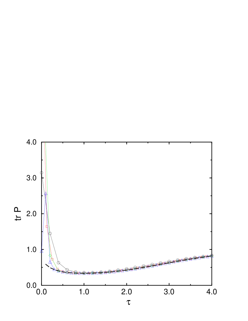
FIG. 1.: Comparison of quantum mechanical traces ($j=10$ (circles), $j=30$ (squares), $j=50$ (diamonds) and $j=80$ (triangles)) with classical trace (thick dashed line) for $k=4.0$, $\beta=2.0$ as function of $\tau$. There are no bifurcations for $\tau\gtrsim 0.1$.

FIG. 2.: The $\mu$–component of the fixed points at $k=8.0$, $\beta=2.0$ as a function of $\tau$. There are four fixed points at $\tau=0.0$ out of which two coincide and disappear at $\tau\simeq 0.57$. A new pair is born at $\tau\simeq 1.89$, but one fixed point disappears again at $\tau\simeq 2.47$, in close vicinity with one of the original fixed points.

FIG. 3.: Strange attractor for $k=8.0$, $\beta=2.0$, $\tau=1.0$. The diamonds mark the position of the two fixed points. The borders $\varphi=\pi$ and $\varphi=-\pi$ have to be identified.

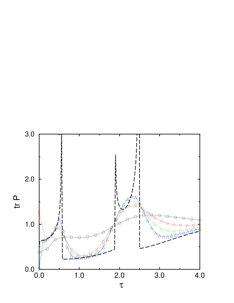
FIG. 4.: Comparison of quantum mechanical traces with classical trace for $k=8.0$, $\beta=2.0$ as a function of $\tau$ (same symbols as in Fig.1). The classical trace diverges whenever a bifurcation is reached.

FIG. 5.: Quantum mechanical and classical trace as a function of $N$ for $k=4.0$, $\beta=2.0$, $\tau=4.0$ (same symbols as in Fig.1). The classical trace is shown as dashed line for better visibility, even though it is only defined for integer $N$. The inset shows that the exponential convergence to 1 also holds in the classical case. The classical dynamics is dominated by a single point–attractor/repeller pair.

FIG. 6.: Quantum mechanical and classical trace as a function of $N$ for $k=8.0$, $\beta=2.0$, $\tau=1.0$ (same symbols as in Fig.1). The corresponding phase space portrait is the strange attractor shown in Fig3.

REFERENCES

- [1] T.Dittrich in Quantum Transport and Dissipation, T. Dittrich, P. Hänggi, G.-L. Ingold, B. Kramer, G. Schön, and W. Zwerger, Wiley–VCH, Weinheim (1998).
- [2] S.Habib, K.Shizume, and W.H.Zurek, Phys.Rev.Lett.80, 4361 (1998).
- [3] D.Cohen, Phys.Rev.Lett.78, 2878 (1997).
- [4] T.Dittrich and R.Graham, Ann.of Phys.200, 363 (1990).
- [5] T.Dittrich and R.Graham, Z.Phys.B 62, 515 (1986).
- [6] R.Graham and T.Tél, Z.Phys.B 60, 127 (1985).
- [7] O.Bohigas, M.J. Giannoni and C.Schmitt, Phys.Rev.Lett 52, 1 (1984).
- [8] M.V.Berry in Les Houches Session XXXVI 1981, Chaotic Behavior of Deterministic Systems, eds. G.Ioss, H.R.Helleman, R.Stora, North–Holland, Amsterdam (1983).
- [9] T.Guhr, A.Müller-Groeling, H.A.Weidenmüller, Phys. Rep. 299,190 (1998).
- [10] L.E.Reichl, The Transition to Chaos, Springer, New York (1992).
- [11] F.Haake, Quantum Signatures of Chaos, Springer, Berlin (1991).
- [12] W.H.Zurek, Phys.Rev.D24, 1516 (1981) and Physics today, 44, No.10, 36 (1991).
- [13] D.Giulini, E.Joos, C.Kiefer, J.Kupsch, I.-O. Stamtescu, and H.D.Zeh, Decoherence and the Appearance of a Classical World in Quantum Theory, Springer, Berlin (1996).
- [14] There are exceptions due to symmetrical couplings, see D.A.Lidar, I.L.Chuang, and K.B.Whaley, Phys.Rev.Lett.81, 2594 (1998); D.Braun, P.Braun, and F.Haake, unpublished.
- [15] P.Pepłowski and S.T.Dembiński, Z.Phys.B 83, 453 (1991);J.Iwaniszewski and P.Pepłowski, J.Phys.A:Math.Gen.28, 2183 (1995).
- [16] A.R.Kolovsky, Phys.Rev.Lett.76, 340 (1996).
- [17] M.G.Gutzwiller, J.Math.Phys.11, 1791 (1970).
- [18] M.G.Gutzwiller, J.Math.Phys.12, 343 (1971).
- [19] P.Cvitanović and B.Eckhardt, J.Phys. A 24. L237 (1991).
- [20] D.Braun, P.A.Braun, and F.Haake, accepted for publication in Physica D (chao-dyn/9804008).
- [21] For a review see U.Weiss, Quantum Dissipative Systems, World Scientific Publishing, Singapore (1993).
- [22] F. Haake, M. Kuś, and R. Scharf: In F. Haake, L.M. Narducci, and D.F. Walls (eds.) Coherence, Cooperation, and Fluctuations, Cambridge University Press, Cambrdge (1986)
- [23] G.S.Agarwal, R.R. Puri, R.P. Singh, Phys. Rev. A56, 2249 (1997) and references therein.
- [24] F.Waldner, D.R.Barberis, H.Yamazaki, Phys. Rev. A 31, 420 (1985).
- [25] R.Bonifacio, P.Schwendimann, and F.Haake, Phys.Rev.A 4, 302 and 854 (1971).
- [26] M.Gross and S.Haroche, Physics Reports (Review Section of Physics Letters), 93, N5, 301-396 (1982)
- [27] P.A.Braun, D.Braun, F.Haake, and J.Weber, Europ.Phys.Journ. D 2, 165 (1998)
- [28] P.A.Braun, D.Braun, and F.Haake, Eur.Phys.J. D 3, 1 (1998).
- [29] M.Tabor, Physica D 6, 195 (1983); G.Junker and H.Leschke, Physica D, 56, 135 (1992).
- [30] P.A.Braun, P.Gerwinski. F.Haake, and H.Schomerus, Z.Phys. B 100, 115 (1996).
- [31] J. H. Van Vleck, Proc. Natn. Acad. Sci. 14, 178 (1928)
- [32] P.Gaspard, Chaos, Scattering and Statistical Mechanics (Cambridge University Press, New York 1988).