Anomalous Scaling in a Model of Hydrodynamic Turbulence with a Small Parameter

Abstract

The major difficulty in developing theories for anomalous scaling in hydrodynamic turbulence is the lack of a small parameter. In this Letter we introduce a shell model of turbulence that exhibits anomalous scaling with a tunable small parameter. The small parameter $\epsilon$ represents the ratio between deterministic and random components in the coupling between $N$ identical copies of the turbulent field. We show that in the limit $N\to\infty$ anomalous scaling sets in proportional to $\epsilon^{4}$. Moreover we give strong evidences that the birth of anomalous scaling appears at a finite critical $\epsilon$, being $\epsilon_{c}\approx 0.6$.

The statistics of the small scale structure of turbulence is characterized by “anomalous scaling” meaning that correlation functions and structure functions of velocity differences across a scale $R$ exhibit a power law behavior with scaling exponents that are not correctly predicted by dimensional analysis. In the last few decades there have been many attempts to compute the scaling exponents of turbulent fields from the equations of motion. In the context of simplified models of passive scalar advection it was discovered that there exist natural small parameters that allow direct computations of anomalous scaling exponents [1, 2, 3]. In Navier Stokes turbulence and also in simplified models like shell models the progress in computing scaling exponents was slowed down by the lack of a small parameter. It is thus worthwhile to consider models of turbulent velocity fields in which a tunable small parameter can be introduced and used to advantage.

We propose to introduce a small parameter via the coupling between $N$ copies of a field $u_{n}$ which satisfies the dynamics of the Sabra shell model of turbulence introduced in [4]:

$${du_{n}(t)\over dt} = i\Big{[}ak_{n+1}~{}u^{*}_{n+1}u_{n+2}+bk_{n}~{}u^{*}_{n-1}u_{n+1}$$ (2)

$$-ck_{n-1}~{}u_{n-2}u_{n-1}\Big{]}-\nu k_{n}^{2}~{}u_{n}+f_{n}(t)\ .$$

Shell models are simplified dynamical systems constructed such that the complex number $u_{n}$ represents the amplitude associated with the Fourier transform of the velocity field ${\mathchoice{{\hbox{\boldmath$\displaystyle u$}}}{{\hbox{\boldmath$\textstyle u$}}}{{\hbox{\boldmath$\scriptstyle u$}}}{{\hbox{\boldmath$\scriptscriptstyle u$}}}}({\mathchoice{{\hbox{\boldmath$\displaystyle r$}}}{{\hbox{\boldmath$\textstyle r$}}}{{\hbox{\boldmath$\scriptstyle r$}}}{{\hbox{\boldmath$\scriptscriptstyle r$}}}})$ with “wave-vector” $k_{n}$. Rather than considering the full $\textstyle k$ space and all the nonlinear interactions one allows for only one-dimensional $k$ vectors on shells spaced such that $k_{n}\equiv k_{0}\lambda^{n}$, with $\lambda$ being the spacing parameter, and local interactions. In Eq. (2) $\nu$ is the “viscosity” and $f_{n}(t)$ a random Gaussian force restricted to the lowest shells. The parameters $a,~{}b$ and $c$ are restricted by the requirement $a+b+c=0$ which guarantees the conservation of the “energy” $E=\sum_{n=0}^{N}|u_{n}(t)|^{2}$ in the in-viscid, unforced limit.

We now want to generalize this model to one which consist of $N$ suitably coupled copies of it. In order to do that we need to consider separately the equations for the real and imaginary parts of $u_{n}$. This procedure guarantees that the obtained model converges to the original Sabra model in the limit $N\to 1$. The copies are indexed by $i,j$ or $\ell$, and these indices take on values $-J,\dots,+J$, $2J+1=N$. The $i$th copy of the velocity field is denoted as $u^{[i]}_{n,\sigma}$. In this notation $\sigma=\pm 1$ refers to the real and imaginary parts of $u_{n}$ respectively. Let $D^{[ij\ell]}$ be the coupling between copies, which will be chosen later. Equations (2) for a collection of copies are

$${du^{[i]}_{n,\sigma}\over dt}=\sum_{j\ell}D^{[ij\ell]}\Big{[}A^{(\sigma)}_{\sigma^{\prime}\sigma^{\prime\prime}}\Big{(}\gamma_{a,n+1}u^{[j]}_{n+1,\sigma^{\prime}}u^{[\ell]}_{n+2,\sigma^{\prime\prime}}$$ (3)

$$\quad+\gamma_{b,n}u^{[j]}_{n-1,\sigma^{\prime}}u^{[\ell]}_{n+1,\sigma^{\prime\prime}}\Big{)}+C^{(\sigma)}_{\sigma^{\prime}\sigma^{\prime\prime}}\gamma_{c,n-1}u^{[j]}_{n-2,\sigma^{\prime}}u^{[\ell]}_{n-1,\sigma^{\prime\prime}}\Big{]}$$ (4)

$$\quad-\nu k_{n}^{2}~{}u^{[i]}_{n,\sigma}+f^{[i]}_{n,\sigma}\ ,$$ (5)

where

$$\gamma_{a,n}\equiv ak_{n}\,,\quad\gamma_{b,n}\equiv bk_{n}\,,\quad\gamma_{c,n}\equiv ck_{n}\ .$$ (6)

and

$${\mathchoice{{\hbox{\boldmath$\displaystyle A$}}}{{\hbox{\boldmath$\textstyle A$}}}{{\hbox{\boldmath$\scriptstyle A$}}}{{\hbox{\boldmath$\scriptscriptstyle A$}}}}^{(+1)}\equiv\left(\begin{array}[]{cc}1&0\\ 0&1\end{array}\right)\ ,\qquad{\mathchoice{{\hbox{\boldmath$\displaystyle A$}}}{{\hbox{\boldmath$\textstyle A$}}}{{\hbox{\boldmath$\scriptstyle A$}}}{{\hbox{\boldmath$\scriptscriptstyle A$}}}}^{(-1)}\equiv\left(\begin{array}[]{cc}0&-1\\ 1&0\end{array}\right)\ ,$$ (11)

$${\mathchoice{{\hbox{\boldmath$\displaystyle C$}}}{{\hbox{\boldmath$\textstyle C$}}}{{\hbox{\boldmath$\scriptstyle C$}}}{{\hbox{\boldmath$\scriptscriptstyle C$}}}}^{(+1)}\equiv\left(\begin{array}[]{cc}-1&0\\ 0&1\end{array}\right)\ ,\quad{\mathchoice{{\hbox{\boldmath$\displaystyle C$}}}{{\hbox{\boldmath$\textstyle C$}}}{{\hbox{\boldmath$\scriptstyle C$}}}{{\hbox{\boldmath$\scriptscriptstyle C$}}}}^{(-1)}\equiv\left(\begin{array}[]{cc}0&1\\ 1&0\end{array}\right)\,,$$ (16)

Note that $A^{(\sigma)}_{\sigma^{\prime}\sigma^{\prime\prime}}=A^{(\sigma^{\prime})}_{\sigma\sigma^{\prime\prime}}\,,\qquad A^{(\sigma)}_{\sigma^{\prime}\sigma^{\prime\prime}}=C^{(\sigma^{\prime})}_{\sigma^{\prime\prime}\sigma}$.

To proceed we note that the index $\ell$ is defined modulo $N$, and introduce a Fourier transform in the “copy” space, defining the collective variables:

$$u^{\alpha}_{n,\sigma}={1\over\sqrt{N}}\sum_{\ell=-J}^{J}u^{[\ell]}_{n,\sigma}\exp\Big{(}{2i\pi\alpha\ell\over N}\Big{)}\ .$$ (17)

Note that the index $\alpha$ is also defined modulo $N=2J+1$. It is convenient to consider values $\alpha$ within “the first Brillouin zone” , i.e from $-J$ to $J$. We will refer to it as the $\alpha$-momentum. Since $u^{[i]}_{n,\sigma}$ is real, $u^{-\alpha}_{n,\sigma}=u^{\alpha\,*}_{n,\sigma}$. In “$\alpha$-Fourier space” Eqs. (5) read

$$\!\!\!\!\!\!\!{du^{\alpha}_{n,\sigma}\over dt}=\sum_{\beta,\gamma}\Phi^{\alpha,\beta,\gamma}[\Delta_{\alpha,\beta+\gamma}+\Delta_{\alpha+N,\beta+\gamma}+\Delta_{\alpha,\beta+\gamma+N}]\,$$ (18)

$$\times \Big{\{}A^{\sigma}_{\sigma^{\prime}\sigma^{\prime\prime}}\big{[}\gamma_{a,n+1}u^{\beta}_{n+1,\sigma^{\prime}}u^{\gamma}_{n+2,\sigma^{\prime\prime}}+\gamma_{b,n}u^{\beta}_{n-1,\sigma^{\prime}}u^{\gamma}_{n+1,\sigma^{\prime\prime}}\big{]}$$ (19)

$$+ C^{\sigma}_{\sigma^{\prime}\sigma^{\prime\prime}}\gamma_{c,n-1}u^{\beta}_{n-2,\sigma^{\prime}}u^{\gamma}_{n-1,\sigma^{\prime\prime}}\Big{\}}-\nu k_{n}^{2}~{}u^{\alpha}_{n,\sigma}+f^{\alpha}_{n,\sigma}\ .$$ (20)

where $\Delta_{\alpha,\beta}$ is the Kronecker symbol. Observe that we use Greek indices for components in $\alpha$-Fourier space, and Latin indices for copies in the copy space. As a consequence of the discrete translation symmetry of the copy index $[i]$ Eqs. (20) conserve $\alpha$-momentum modulo $N$ at the nonlinear vertex, as one can see explicitly in the above equation. The coupling amplitudes $\Phi^{\alpha,\beta,\gamma}$ in these equations are the Fourier transforms of the amplitudes $D^{[ij\ell]}$.

We choose the coupling amplitudes according to

$$\Phi^{\alpha,\beta,\gamma}={1\over\sqrt{N}}\big{[}\epsilon+\sqrt{1-\epsilon^{2}}\,\Psi^{\alpha,\beta,\gamma}\big{]}\;,$$ (21)

where $\Psi^{\alpha,\beta,\gamma}$ are quenched random phases, uniformly and independently distributed with zero average (cf. the “Random Coupling Model” (RCM) for the Navier-Stokes statistics [5] and the identical symmetry conditions there). Consequently for $\epsilon=0$ the model reduces to the RCM and exhibits normal scaling (K41) for $N\to\infty$. It was in fact understood [5, 6] that in the limit $N\to\infty$ the direct interaction approximation (DIA) becomes the exact solution of the RCM. Moreover a proper analysis of the DIA approximation leads to normal scaling for those systems in which sweeping effects are removed or absent by construction like in shell models [7, 6].

On the other hand for $\epsilon=1$ the coupling coefficients in the $\alpha$-Fourier space (21) are index-independent. This corresponds to uncoupled Eqs. (5) in the copy space, because in this case $D^{[ij\ell]}=\delta_{i,j}\delta_{i,\ell}$. Thus for $\epsilon=1$ we recover the original Sabra model with anomalous scaling[4]. Our choice of couplings (21) allows an interpolation between the normal K41 scaling for $\epsilon=0$ (at $N\to\infty$) and the full anomalous scaling of Sabra model for $\epsilon=1$. A model of this type was proposed in the context of Navier-Stokes statistics by Kraichnan in [8] and analyzed by Eyink [6] in terms of perturbative expansions.

Our aim in this Letter is to present numerical results which show that for small values of $\epsilon$ the model exhibits small anomalous corrections to normal scaling and to present theoretical arguments to rationalize the functional dependence of the anomalous corrections on $\epsilon$. We measured the scaling exponents of the structure functions:

$$S_{2p}(k_{n})\equiv\frac{1}{N}\langle\sum_{i=-J}^{J}\sum_{\sigma}|u^{[i]}_{n,\sigma}|^{2p}\rangle\sim k_{n}^{-\zeta_{2p}}\;.$$ (22)

The exponents $\zeta_{2p}$ have been calculated by a linear fit in the two decades inertial range, see Fig. 1. The equations of motion (20) with 28 shells, $a=1$, $b=c=-0.5$, were integrated with the slaved Adams-Bashforth algorithm, viscosity $\nu=4\times 10^{-9}$, a time-step $\Delta t=10^{-5}$. The forcing was subjected on the first two shells, chosen random Gaussian with zero average and with variances such that $\sigma_{2}/\sigma_{1}=0.7$ (in order to minimize the input of helicity[4] which leads to period two oscillation in the structure

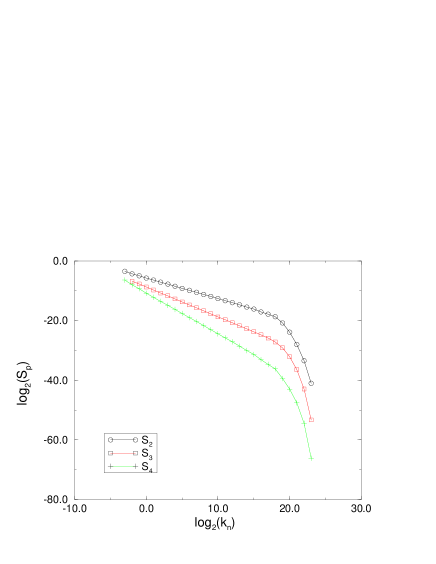
FIG. 1.: Log-log plot of the structure functions $S_{p}(k_{n})$ vs $k_{n}$ for p=2,3,4, $\epsilon=0.8$ and $N=25$.

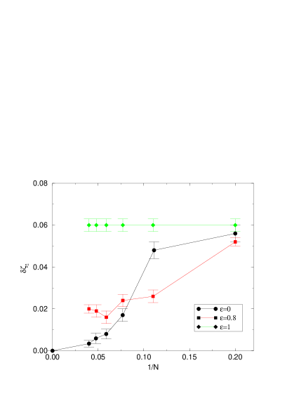
FIG. 2.: $\delta\zeta_{2}=\zeta_{2}-2/3$ vs $1/N$ for $\epsilon=0$ (circles), $\epsilon=0.8$ (squares) and $\epsilon=1$ (diamonds) for $N$ from 5 to 25. The point at $1/N=0$ for the $\epsilon=0$ curve is the theoretical prediction of the RCM for $N\to\infty$.

functions). Averages were taken for a time equal to 250 eddy turnover times for the case $N=1$. The averaging times were decreased when the number of copies increased, taking into account the faster convergence times in these cases. The quality of the scaling behavior and of the fits is demonstrated in Fig. 1.

To substantiate the birth of anomalous scaling at $\epsilon>0$ we simulated the model for different values of $\epsilon$ and of $N$. We are interested in the values of the scaling exponents for very large values of $N$ ($\infty$ in theory). In Fig. 2 one can see the plot of the value of the anomalous corrections to Kolmogorov scaling, $\delta\zeta_{2}=\zeta_{2}-2/3$, as function of $1/N$ for $\epsilon=0.8$ together with the same curve for $\epsilon=0$ and for $\epsilon=1$ for $N$ ranging from 5 to 25. While for $\epsilon=0$ the corrections to Kolmogorov scaling go to zero, for $\epsilon=0.8$ and for $\epsilon=1$ the corrections converge to a finite value which increases with $\epsilon$.

FIG. 3.: $\delta\zeta_{2}=\zeta_{2}-2/3$ vs $\epsilon^{4}$ (circles), vs $\epsilon^{2}$ (squares) and vs $\epsilon$ (diamonds) together with linear, quadratic and quartic fits respectively for N=25.

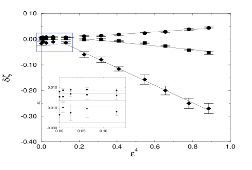
FIG. 4.: $\delta\zeta_{2}=\zeta_{2}-2/3$ (circles), $\delta\zeta_{4}$ (squares) and $\delta\zeta_{6}$ (diamonds) vs $\epsilon^{4}$ for $N=25$.

The random phases in the couplings were chosen with respect to a uniform probability with zero-mean at the beginning of each simulation. The rigorous procedure for quenched disorder would call for taking averages over different runs with different choices of the couplings. We did not do that, but rather checked that self-averaging is already valid for $N=5$, for $\epsilon=0.8$ (small random component in the couplings) and within our numerical precision. For $\epsilon=0$ self-averaging occurs only for large numbers of copies.

The most interesting aspects of the numerical findings are the dependence of the anomalies on $\epsilon$ and the question whether anomaly appears for any $\epsilon>0$ or only above a critical value $\epsilon_{c}$. The first issue is settled with sufficient clarity in Fig. 3 in which we show the behavior of $\delta\zeta_{2}$ (for N=25) as a function of $\epsilon$, $\epsilon^{2}$ and $\epsilon^{4}$ with the respective linear, quadratic and quartic fits. One can see clearly that the anomalous corrections $\delta\zeta_{2}$ go to zero like $\epsilon^{4}$. The same behavior is exhibited by $\delta\zeta_{4}$ and $\delta\zeta_{6}$ as one can see in Fig  4.

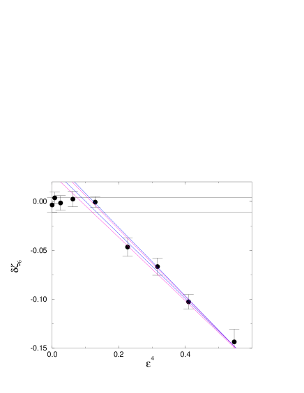
FIG. 5.: $\delta\zeta_{6}=\zeta_{6}-2$ vs $\epsilon^{4}$ for $N=25$ with the maximal and minimal slope lines obtained for the linear fits in the two ranges $\epsilon^{4}\in[0.13,0.88]$ and $\epsilon^{4}\in[0.23,0.88]$ . All the values of the anomalous corrections have been shifted by the average of the first five points.

The existence of a critical value $\epsilon_{c}$ is harder to settle. In the following we show arguments in favor of the existence of a finite $\epsilon_{c}$. First one should notice in the magnification in Fig. 4 that at $\epsilon=0$ we do not get the K41 values $\delta\zeta_{n}=0$ as theoretically predicted. This is a result of the finiteness of the number of copies ($N=25$ in Fig. 4).

To establish the existence of a finite $\epsilon_{c}$ we proceeded as follows: i) To take this into account the finite size effects we subtracted the $\epsilon=0$ value of $\delta\zeta_{n}$ from all the values of $\zeta_{n}$. ii) We calculated the maximal and minimal slope line, that is the best fit slope plus and minus the standard deviation, for $\delta\zeta_{n}$ vs $\epsilon^{4}$ in two different ranges: $\epsilon^{4}\in[0.13,0.88]$ and $\epsilon^{4}\in[0.23,0.88]$: that is, we fitted with the 2 parameter function $f(\epsilon^{4})=a_{n}+b_{n}\epsilon^{4}$. iii) We fitted the plot of $\delta\zeta_{n}$ vs $\epsilon$ with the 4 parameter function $g(\epsilon)=a_{n}\epsilon+b_{n}\epsilon^{2}+c_{n}\epsilon^{3}+d_{n}\epsilon^{4}$ in the range $\epsilon\in[0,0.97]$.Note that with the “calibration” of the zero that we performed $\delta\zeta_{n}=0$ for $\epsilon=0$. The $\chi^{2}$ test is much better for the first procedure than for the second, where the minimal $\chi^{2}$ is tripled, although in principle it should be easier to fit a function with a larger number of parameters.

$\delta\zeta_{n}$	range of $\epsilon^{4}$	slope$\times 10^{3}$	$\epsilon_{c}$
$\delta\zeta_{2}$	[0.13,0.88]	48$\pm$ 3	0.60 $\pm$ 0.07
$\delta\zeta_{2}$	[0.23,0.88]	50$\pm$ 3	0.62 $\pm$ 0.06
$\delta\zeta_{4}$	[0.13,0.88]	$-74\pm 8$	0.69 $\pm$ 0.07
$\delta\zeta_{4}$	[0.23,0.88]	$-82\pm 9$	0.71 $\pm$ 0.06
$\delta\zeta_{6}$	[0.13,0.88]	$-341\pm 8$	0.59 $\pm$ 0.04
$\delta\zeta_{6}$	[0.23,0.88]	$-335\pm 6$	0.57 $\pm$ 0.05

TABLE I.: Results of the linear fits on different ranges for different scaling exponents. The values of $\epsilon_{c}$ have been calculated as explained in the body of the text.

We interpret this result as an evidence for the existence of a finite $\epsilon_{c}$.

In order to have a better estimate of the “zero” level of $\delta\zeta_{n}$’s, and so a better estimate of $\epsilon_{c}$, instead of subtracting the value of the anomalous correction at $\epsilon=0$ we subtracted the average value of $\delta\zeta_{n}$ calculated by using the first 5 points belonging to the flat region. The value of $\epsilon_{c}$ with its error has been found by looking at the intersections of the minimal and maximal slope lines with the zero line: the line of the value of $\delta\zeta_{n}$ for $\epsilon=0$ with its error (see Fig. 5). Table I exhibits the resulting values for the various exponents and their linear fits. Note that all the values of $\epsilon_{c}$ coincide within the error bars.

To understand the linear dependence on $\epsilon^{4}$ we turn to the exact equations that are satisfied by the $n$-order correlation functions, which are defined as suitable averages over time and over all the replica. The second and third order correlation functions are defined as:

$$F_{2}(k_{n};t-t^{\prime})\equiv\frac{1}{N}\sum_{\alpha,\sigma}\langle u_{n,\sigma}^{\alpha}(t)u_{n,\sigma}^{\alpha*}(t^{\prime})\rangle\,,$$ (23)

$$F_{3}(k_{n};t,t^{\prime},t^{\prime\prime})\equiv\frac{1}{N}\sum_{\alpha,\alpha^{\prime},\alpha^{\prime\prime}}\sum_{\sigma,\sigma^{\prime},\sigma^{\prime\prime}}\Phi^{\alpha^{\prime\prime},\alpha^{\prime},\alpha}$$ (24)

$$\big{[}\Delta_{\alpha+\alpha^{\prime},\alpha^{\prime\prime}}+\Delta_{\alpha+\alpha^{\prime},\alpha^{\prime\prime}+N}+\Delta_{\alpha+\alpha^{\prime}+N,\alpha^{\prime\prime}}\big{]}$$ (25)

$$\langle u_{n-1,\sigma^{\prime}}^{\alpha}(t)u_{n,\sigma^{\prime}}^{\alpha^{\prime}}(t^{\prime})u_{n+1,\sigma^{\prime\prime}}^{\alpha^{\prime\prime}*}(t^{\prime\prime})\rangle\ .$$ (26)

and similarly for higher order correlation functions and for the response functions (for details see [9]).

The equations of motion for these objects can be written down explicitly. For example,

$${\partial\over\partial t}F_{2}(k_{n},t)=\gamma_{a,n+1}F_{3}(k_{n+1};0,t,t)+\gamma_{b,n}F_{3}(k_{n};t,0,t)$$ (27)

$$+\gamma_{c,n-1}F_{3}(k_{n-1};t,t,0)\,,$$ (28)

$${\partial\over\partial t_{1}}F_{3}(k_{n},t_{1},t_{2},t_{3})=\gamma_{a,n}F_{4}(k_{n},k_{n+1},k_{n},k_{n+1};t_{1},t_{1},t_{2},t_{3})$$ (29)

$$+\gamma_{b,n-1}F_{4}(k_{n-2},k_{n},k_{n},k_{n+1};t_{1},t_{1},t_{2},t_{3})$$ (30)

$$+\gamma_{c,n-2}F_{4}(k_{n-3},k_{n-2},k_{n},k_{n+1};t_{1},t_{1},t_{2},t_{3})\,,$$ (31)

In order to close such equations and to attempt to solve them, one needs to express a higher order correlation function in terms of lower order statistical objects. In [9] it was shown that this can be done in the present context in a controlled fashion. In other words, it is possible to express, say, $F_{4}$ in terms of $F_{2}$, $F_{3}$ and second and third order response functions. In doing so one of course leaves out information about $F_{4}$ that cannot be possibly represented in terms of lower order objects. Yet, the main result of the analysis of [9] is that the neglected terms in this procedure are of $O(\epsilon^{6})$ whereas the retained terms are of $O(1)$ and of $O(\epsilon^{4})$! Since we understand that for $\epsilon=0$ the anomaly must vanish, we expect the anomalies to be proportional to $\epsilon^{4}$. We interpret therefore the numerical results shown in Fig  3 and Fig  4 as an excellent confirmation of this theoretical expectation.

To summarize: we introduced a shell model of hydrodynamic turbulence in which a small tunable parameter $\epsilon$ exists. We know from theoretical and numerical results that the model exhibits normal scaling for $\epsilon=0$. The most important results of this letter are the existence of a finite $\epsilon_{c}$ at which anomalous scaling appears and the behavior as $\epsilon^{4}$ of the anomalous corrections for $\epsilon>\epsilon_{c}$.

REFERENCES

[1]
K. Gawedczki and A. Kupiainen, Phys. Rev. Lett. 75, 3834 (1995)
[2]
M. Chertkov, G. Falkovich, I. Kolokolov and V. Lebedev, Phys. Rev. E 52,
4924 (1995)
[3]
O. Gat, I. Procaccia and R. Zeitak, Phys. Rev. Lett. 80, 5536 (1998).
[4]
V.S. L’vov, E. Podivilov, A. Pomyalov, I. Procaccia and D. Vandembrouq,
Phys. Rev. E, 58 1811 (1998).
[5]
R. H. Kraichnan, J. Math. Phys. 2, 124 (1961).
[6]
G. L. Eyink, Random Coupling Model and Self-Consistent
-Expansion Method, (unpublished).
[7]
D. Pierotti, Europhys. Lett. 37, 323 (1997).
[8] R. H. Kraichnan, J. Fluid Mech. 41 189 (1970).
[9]
V.S. L’vov, D. Pierotti, A. Pomyalov, I. Procaccia,
submitted to Phys. Fluids, special issue in Honour
of R.H. Kraichnan (1998).