Escape from intermittent repellers-
Periodic orbit theory for crossover from exponential to algebraic decay

Abstract

We apply periodic orbit theory to study the asymptotic distribution of escape times from an intermittent map. The dynamical zeta function exhibits a branch point which is associated with an asymptotic power law escape. By an analytic continuation technique we compute a zero of the zeta function beyond its radius of convergence leading to a pre-asymptotic exponential decay. The time of crossover from an exponential to a power law is also predicted. The theoretical predictions are confirmed by numerical simulation. Applications to conductance fluctuations in quantum dots are discussed.

I Introduction

Exponential distribution of escape times from chaotic scattering systems should be expected only if the associated repeller is hyperbolic. For intermittent repellers one expects asymptotic power law decay[1, 2]. Nevertheless, in numerical simulations one often observes what appears to be a perfect exponential[3, 4], and an expected crossover to a power law may be hard to detect, because it may occur after a long time where it is difficult to obtain descent statistics.

The importance of intermittency cannot be overemphasized. A generic Hamiltonian system exhibits a mixed phase space structure. A typical trajectory is intermittently trapped close to the stable islands [5]. But even fully chaotic billiards may exhibit intermittency, typically if they have neutrally stable orbits. Popular billiards such as the Stadium and the Sinai billiards are of this type.

A quantum dot is an open scattering system in two dimensions, obtained by connecting leads to a cavity. Inspired by Quantum Chaos research, one likes to contrast shapes of the cavity corresponding to chaotic motion, like the stadium, with shapes corresponding to integrable motion, like the rectangle or the square. Both extreme cases are sensitive to naturally occurring imperfections and one naturally ends up with mixed phase space systems where one component hopefully dominates. Consequently, the signals of underlying chaos or integrability don’t show up as clear cut as one would have hoped for.

Much of the analysis of these problems has been numerical and heuristic. To strengthen the theoretical analysis we will, in this paper, apply periodic orbit theory and cycle expansions to make quantitative predictions concerning the asymptotic distribution of escape times from an intermittent map. We will demonstrate that a pre-asymptotic exponential escape law is associated with a pair of complex conjugate zeroes of the zeta function beyond its domain of convergence. This zero will be computed with a simple resummation technique[6]. The truly asymptotic escape distribution will be a power law, and is associated with a branch point of the zeta function. The strength of this power law will also be provided by the resummation scheme, whereas the particular power is known from analytic argument for our particular model system. The relative magnitudes of the pre-exponential and the power law will yield a good estimate of the cross over time, which will be surprisingly high.

II Escape and periodic orbits

Much of the early work on cycle expansion [7] was concerned with escape from (hyperbolic) repellers, so we can follow ref. [7] rather closely when deriving the basic formulas relating escape to the periodic orbits of the repeller.

Consider a 1-d map, on some interval $I$, with $L$ monotone branches $f_{i}(x)$ where $1\leq i\leq L$. Each branch $f_{i}(x)$ is defined on an interval $I_{i}$. A generating partition is then given by ${\cal C}^{(1)}=\{I_{1},I_{2}\ldots I_{L}\}$. We want the map to admit an unrestricted symbolic dynamics. We therefore require all branches to map their domain $f_{i}(I_{i})=I$ onto some interval $I\supset{\cal C}^{(1)}$ covering ${\cal C}^{(1)}$. A trajectory is considered to escape when some iterate of the map $x\notin{\cal C}^{(1)}$.

The $n$’th level partition ${\cal C}^{(n)}=\{I_{q};n_{q}=n\}$ can be constructed iteratively. Here $q$ are words of length n built from the alphabet ${\cal A}=\{i;0\leq i\leq L\}$. An interval is thus defined recursively according to

$$I_{iq}=f_{i}^{-1}(I_{q})\ \ ,$$ (1)

where $iq$ is the concatenation of letter $i$ with word $q$. A concrete example will be given in eq. (16) and fig. 1. Next define the characteristic function for the $n$’th level partition

$$\chi^{(n)}(x)=\sum_{q}^{(n)}\chi_{q}(x)\ \ ,$$ (2)

where

$$\chi_{q}(x)=\left\{\begin{array}[]{cc}1&x\in I_{q}\\ 0&x\notin I_{q}\end{array}\right.\ \ .$$ (3)

An initial point surviving $n$ iterations must be contained in ${\cal C}^{(n)}$. Starting from an initial (normalized) distribution $\rho_{0}(x)$ we can express the fraction that survives $n$ iterations as

$$\Gamma_{n}=\int\rho_{0}(x)\chi^{(n)}(x)dx\ \ .$$ (4)

We choose the distribution $\rho_{0}(x)$ to be uniform on the interval $I$. The survival probability is then given by

$$\Gamma_{n}=a\sum_{q}^{(n)}|I_{q}|\ \ ,$$ (5)

where

$$a^{-1}=\int_{I}dx=|I|\ \ .$$ (6)

Assuming hyperbolicity the size of $I_{q}$ can be related to the stability $\Lambda_{q}=\frac{d}{dx}f^{n}(x)\mid_{x\in q}$ of periodic orbit $\overline{q}$ according to

$$|I_{q}|=b_{q}\frac{1}{|\Lambda_{q}|}$$ (7)

where $b_{q}=O(|I|)$, can be bounded close to the size of $I$. This results from the fact that $f^{n}(I_{q})=I$, the smallness of $|I_{q}|$ and the fact that derivatives can be bounded due to hyperbolicity. We will eventually relax the assumption of hyperbolicity, but for the moment we’ll stick to it.

The survival fraction can now be bounded by the periodic orbit sum according to

$$C_{1}(N)\;\sum_{q}^{(n)}\frac{1}{|\Lambda_{q}|}<\Gamma_{n}<C_{2}(N)\;\sum_{q}^{(n)}\frac{1}{|\Lambda_{q}|}$$ (8)

for all $n>N$. For large $N$ (and assuming hyperbolicity) $C_{1}(N)$ and $C_{2}(N)$ can be chosen close to unity.

The periodic orbit sum in (8) will be denoted $Z_{n}$

$$\sum_{q}^{(n)}\frac{1}{|\Lambda_{q}|}\equiv Z_{n}\ \ .$$ (9)

and can be rewritten as a sum over primitive periodic orbits (period $n_{p}$) and their repetitions

$$Z_{n}=\sum_{p}n_{p}\sum_{r=1}^{\infty}\frac{\delta_{n,r\;n_{p}}}{|\Lambda_{p}|^{r}}\ \ .$$ (10)

It is closely related to the trace of the Perron-Frobenius operator

$$Z_{n}\approx\mbox{tr}{\cal L}^{n}=\int dx\delta(x-f^{n}(x))=\sum_{p}n_{p}\sum_{r=1}^{\infty}\frac{\delta_{n,r\;n_{p}}}{|\Lambda^{r}_{p}-1|}\ \ .$$ (11)

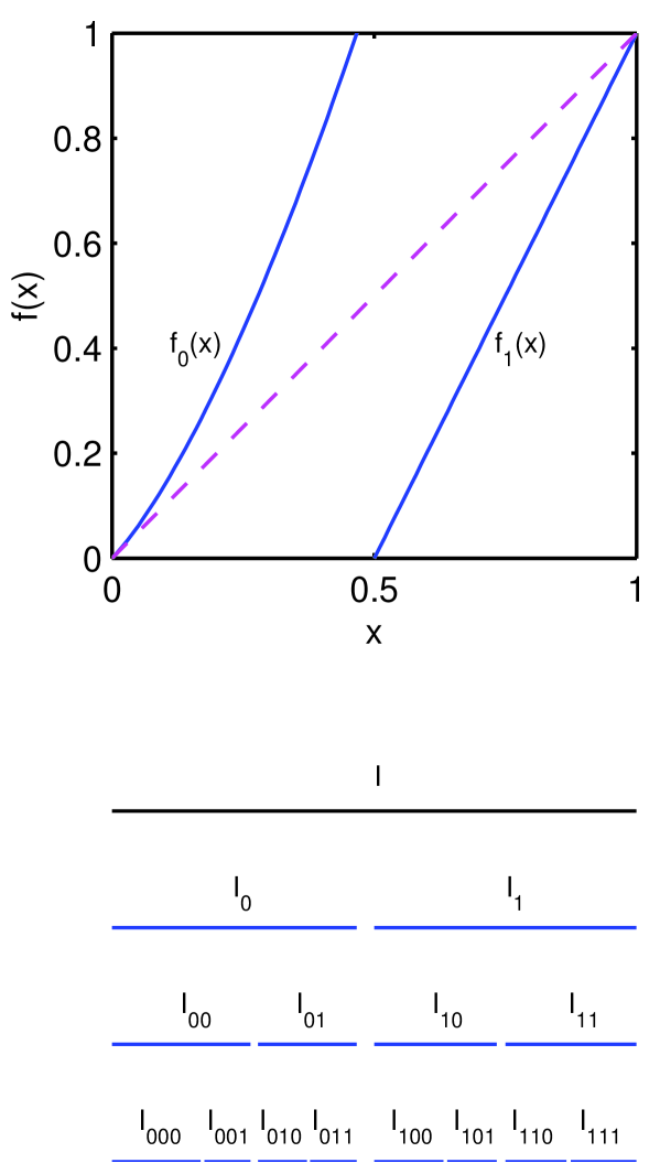
FIG. 1.: The intermittent map (16) for the parameter values $s=0.7$ and $p=1.2$. The map is defined on the interval $I$. Below the map is also shown the partitions ${\cal C}^{(1)}=\{I_{0},I_{1}\}$, ${\cal C}^{(2)}$ and ${\cal C}^{(3)}$.

By introducing the zeta function

$$\zeta^{-1}(z)=\prod_{p}\left(1-\frac{z^{n_{p}}}{|\Lambda_{p}|}\right)\ \ ,$$ (12)

the periodic orbit sum $Z_{n}$ can be expressed as a contour integral

$$Z_{n}=\frac{1}{2\pi i}\int_{\gamma}z^{-n}\left(\frac{d}{dz}\log\zeta^{-1}(z)\right)dz\ \ ,$$ (13)

where the small contour $\gamma$ encircles the origin in negative direction.

The expansion of the zeta function to a power series is usually referred to as a cycle expansion.

$$\zeta^{-1}(z)=\sum c_{n}z^{n}\ \ .$$ (14)

This representation converges up to the leading singularity, unlike the product representation (12) which diverges at (nontrivial) zeroes. If the zeta function $\zeta^{-1}(z)$ is analytic in a disk extending beyond the leading zero $z_{0}$, then the periodic orbit sum $Z_{n}$, and hence the survival probability $\Gamma_{n}$, will decay asymptotically as

$$Z_{n}\sim z_{0}^{-n}\equiv e^{-\kappa n}$$ (15)

where $\kappa=\log z_{0}$ is the escape rate.

We will introduce intermittency in connection with a specific model. We then consider an intermittent map $x\mapsto f(x)$ with two branches $L=2$, and where $I$ is chosen as the unit interval:

$$f(x)=\left\{\begin{tabular}[]{lll}$f_{0}(x)=x\left(1+p\;(2x)^{s}\right)$&$x\in I_{0}=\{x;0\leq x<\xi\}$\\ $f_{1}(x)=2x-1$&$x\in I_{1}=\{x;1/2\leq x\leq 1\}$\end{tabular}\ \ ,\right.$$ (16)

The map is intermittent if $s>0$ and allows escape if $p>1$. The map is shown in fig. 1, together with some of its partitions. The right edge of the left branch $I_{0}$, denoted $\xi$, is implicitly defined by $f_{0}(\xi)=1$. The particle is considered to escape if $\xi(s)<x<\frac{1}{2}$.

The intermittent property is related to the fact that the cycle $\overline{0}$ is neutrally stable $f^{\prime}(0)=1$. Consequently, cycle stabilities can no longer be exponentially bounded with length. This loss of hyperbolicity makes it difficult to relate the survival probability $\Gamma_{n}$ to the periodic orbit sums $Z_{n}$. Indeed, eq. (7) is brutally violated in some cases, as can been realized from the following example. The problem of intermittency is best represented by the family of periodic orbits $10^{k}$. It follows from eqs. (1) and (16) that $|I_{10^{k}}|=\frac{1}{2}|I_{0^{k}}|$. It can be shown [6] that $|I_{0^{k}}|\sim\frac{1}{k^{1/s}}$ and thus

$$|I_{10^{k}}|\sim\frac{1}{k^{1/s}}$$ (17)

which should be compared with the asymptotic behavior of the stabilities

$$1/\Lambda_{10^{k}}\sim\frac{1}{k^{1+1/s}}$$ (18)

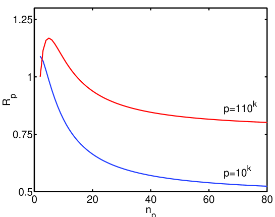
FIG. 2.: The quantity $R_{p}$ plotted for the sequences $p=10^{k}$ and $p=110^{k}$ versus length $n_{p}$.

The difference in power laws seems to spoil every possibility of a bound like (8). However, eq. (7) is not necessary for that purpose. It suffices if the ratio

$$R_{p}=\frac{|\Lambda_{p}|}{n_{p}}\sum_{k=1}^{n_{p}}|I_{{\cal S}^{k}p}|$$ (19)

stays bounded. That it to say that it suffices if the average size of the intervals along a cycle can be related to the stability, rather than each interval separately. Here ${\cal S}$ denotes the shift operator. We check this numerically on two sequences: $10^{k}$ and $110^{k}$, the former being most sensitive to intermittency. The result is plotted in fig. 2. We note that for both sequences, $R_{p}$ appear to tend to well defined limits, where $10^{k}$ lead to the largest deviation from unity. Indeed, it is reasonable to assume that the sequence $10^{k}$ provides a lower bound

$$R_{p}>\lim_{k\rightarrow\infty}R_{10^{k}}\hskip 22.76228pt\forall p\ \ .$$ (20)

In view of this, the numerical results strongly suggest that $R_{p}$ stays bounded, and that, for this particular system, $C_{1}$ in eq. (8) can be chosen as $C_{1}=0.5$ and $C_{2}$ presumably close to unity. This is a surprisingly low price to pay for the complication of intermittency.

The sizes of the intervals $I_{0^{n}}$ has no relation whatsoever to the stability of the cycle $\overline{0}$, which is unity. We exclude the intervals $I_{0^{n}}$ from our considerations by pruning the fixpoint from the zeta function

$$\zeta^{-1}(z)=\prod_{p\neq 0}\left(1-\frac{z^{n_{p}}}{|\Lambda_{p}|}\right)\ \ ,$$ (21)

The contribution from $I_{0^{n}}$ to $\Gamma_{n}$ can be added separately if required.

Since the result rely on summation along periodic orbits, it might break down for some choices of the initial distribution $\rho_{0}(x)$ were such a summation is not carried out.

III Resummation and simulation

After having argued that the survival probability $\Gamma_{n}$ still can be bounded close to periodic orbit sums $z_{n}$ we turn to the problem of computing the asymptotics of these periodic orbit sums. The coefficients of the cycle expansion (14) for the map (16) decay asymptotically as

$$c_{n}\sim\frac{1}{n^{1+1/s}}\ \ ,$$ (22)

which induces a singularity of the type $(1-z)^{1/s}$ in the zeta function [6]. If $1/s$ is an integer, the singularity is $(1-z)^{1/s}\log(1-z)$.

To evaluate the periodic orbit sum it is convenient to consider a resummation of the zeta function around the branch point $z=1$.

$$\zeta^{-1}(z)=\sum_{i=0}^{\infty}c_{i}z^{i}=\sum_{i=0}^{\infty}a_{i}(1-z)^{i}+(1-z)^{1/s}\sum_{i=0}^{\infty}b_{i}(1-z)^{i}\ \ .$$ (23)

In practical calculations one has only a finite number of coefficients $c_{i}$, $0\leq i\leq n_{c}$ of the cycle expansion at disposal. Here $n_{c}$ is the cutoff in (topological) length. In [6] we proposed a simple resummation scheme for the computation of the coefficients $a_{i}$ and $b_{i}$ in (23). We replace the infinite in (23) sums by finite sums of increasing degrees, $n_{a}$ and $n_{b}$, and require that

$$\sum_{i=0}^{n_{a}}a_{i}(1-z)^{i}+(1-z)^{1/s}\sum_{i=0}^{n_{b}}b_{i}(1-z)^{i}=\sum_{n=0}^{n_{c}}c_{n}z^{n}+O(z^{n+1})\ \ .$$ (24)

One expands $(1-z)^{i(+1/s)}$ in binomial sums (series). If $n_{a}+n_{b}+2=n+1$ this leads to a solvable linear system of equations yielding the coefficients $a_{i}$ and $b_{i}$. It is natural to require that $|n_{a}+\frac{1}{s}-n_{b}|<1$ so that the maximal powers of the two sums in eq. (24) are adjacent.

If the zeta function is entire in the entire $z$ plane (except for the branch cut) the periodic orbit sum can be written

$$Z_{n}=\sum_{\alpha}z_{\alpha}^{-n}+\frac{1}{2\pi i}\int_{\gamma_{cut}}z^{-n}\left(\frac{d}{dz}\log\zeta^{-1}(z)\right)dz\ \ .$$ (25)

The sum is over all zeroes $z_{\alpha}$ of the zeta function (assuming they are not degenerated) and the contour $\gamma_{cut}$ goes round the branch cut in positive direction. If poles and/or natural boundaries are present, expression (25) must be accordingly modified.

The leading asymptotic behavior is provided by the vicinity of the branch point $z=1$, and is found to be [8]

$$Z_{n}\sim\frac{b_{0}}{a_{0}}\frac{1}{s}\frac{1}{\Gamma(1-1/s)}\frac{1}{n^{1/s}}\hskip 28.45274ptn\rightarrow\infty\ \ .$$ (26)

The relevant ratio $b_{0}/a_{0}$, obtained from the resummation scheme, versus cutoff length $n_{c}$ is plotted in fig. 3. In all numerical work we have used the parameters $s=0.7$ and $p=1.2$. and computed all periodic orbits up to length 20.

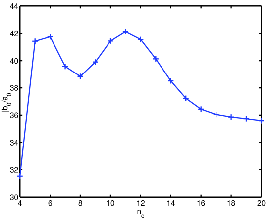
FIG. 3.: The ratio $b_{0}/a_{0}$ versus cutoff length $n_{c}$.

There is also a pair of complex conjugate zeroes, $z_{0}=x_{0}\pm iy_{0}$ close to the branch cut. They contribute both to the sum over zeroes and to the integral around the cut in (25). But since their imaginary part $y_{0}$ is small, they will, in effect, contribute a factor $x_{0}^{-n}$ to the periodic orbit sum $Z_{n}$.

This zero will dominate $Z_{n}$ in some range $0\ll n\ll n_{cross}$ before the asymptotic power law sets in.

In fig. 4 we study the convergence of the real and imaginary part of $z_{0}$ obtained from the resummation scheme above, for different cutoffs $n_{c}$. The zero is computed by Newton-Raphson iteration of the left hand side of (24), after the resummation has been done. Again we note that the analytic continuation technique works quite satisfactorily.

The probability of escaping at iteration $n$ is

$$p_{n}=\Gamma_{n-1}-\Gamma_{n}\ \ .$$ (27)

We get for this distribution

$$p_{n}\approx\left\{\begin{array}[]{ll}x_{0}^{-n}&0\ll n\ll n_{cross}\\ \frac{b_{0}}{a_{0}}\frac{1}{s^{2}}\frac{1}{\Gamma(1-1/s)}\frac{1}{n^{1+1/s}}&n_{cross}\ll n\end{array}\right.\ \ .$$ (28)

Here we have neglected the interval $I_{0^{n}}$, having the same asymptotic decay law as the periodic orbit sum $Z_{n}$. Due to the uncertainty in the bounds (8) it can be neglected.

The crossover $n=n_{cross}$ takes place when the two terms in (28) are of comparable magnitude. For our standard set of parameters ($p=1.2$, $s=0.7$) it is found to be $n_{cross}\approx 300$.

FIG. 4.: The real and imaginary part of $\log z_{0}$ versus cutoff length $n_{c}$.

The check our predictions we run a simulation of the system. The result can be seen in fig. (5). We note that the slope of the exponential, the power and magnitude of the power law, as well as the crossover time agrees very well with our predictions.

A reader still in any doubt on the effectiveness of cycle expansions should consider the following. The simulation in fig. 5 averaged over $10^{8}$ initial point, yet, in itself the result would not very conclusive. A direct evaluation of the periodic orbit sum up to say $n=600$ would require roughly $10^{170}$ periodic orbits. We have not bothered to perform such a cross check! But a resummed cycle expansion provides reliable answers with a length cutoff as low as $n=15$, corresponding to $4719$ prime cycles. Admittedly, we benefitted from knowing the asymptotic power law of the cycle expansion. However, if this is not the situation, this power law is easily extracted if one uses stability ordering [8].

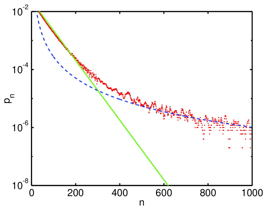
FIG. 5.: Distribution of escape times obtained from simulation (shaky curve) and the pre exponential (full line) and the asymptotic power law (dashed line) obtained from resummation.

IV A zero is cut in two

The occurrence of a dominating zero beyond the branch point is, in fact, very natural. Consider the one-parameter family of zeta functions.

$$\zeta^{-1}(z;\beta)=\prod_{p}\left(1-\frac{z^{n_{p}}}{|\Lambda_{p}|^{\beta}}\right)\ \ .$$ (29)

For $\beta$ small enough there is a leading zero $z_{0}(\beta)$ within the domain of convergence $|z_{0}(\beta)|<1$. This is related to the topological pressure [9, 10] according to ${\cal P}(\beta)=-\log z_{0}(\beta)$. For instance ${\cal P}(0)$ is the topological entropy. For a certain $\beta$ (actually the fractal dimension of the repeller) the zero collides with the branch point $z=1$, splits into two, and continue to move out beyond the branch point.

In fig. 6 we plot the logarithm of the leading zero ($-\log z_{0}(\beta)$) versus $\beta$. It is obtained from a resummation analogous to the one discussed above, cf.[6]. It can be interpreted as the topological pressure only as long it is real.

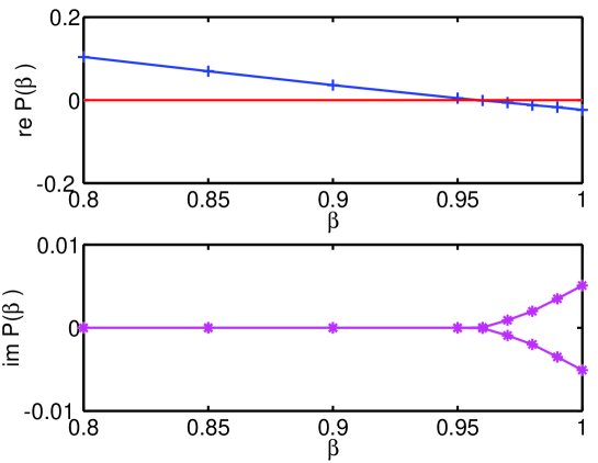
FIG. 6.: The real and imaginary part of the leading zero versus the thermodynamic parameter $\beta$

V Mesoscopic discussion

The particular form of the distribution of escape times does depend on the initial distribution $\rho_{0}(x)$. In this paper we have restricted ourselves to a uniform initial distribution. To model chaotic scattering one must imagine that particles can be injected according to any distribution. For example, one can construct a chaotic scatterer from a bounded billiard by drilling holes wherever on the boundary and injecting particles from different angles. This may even effect the asymptotic power law [11]. Periodic orbit theories can also account for other initial distributions than uniform. However, the preceding discussions about relating periodic orbit sums to survival probabilities warns us to be cautious when doing so for intermittent systems.

As it appears, the general rule of thumb, first an exponential, then a cross over to some powerlaw, can be extended to open Hamiltonian systems with a mixed phase space structure [2, 11].

An immediate application concerns conductance fluctuations in quantum dots [12]. The Fourier transform $\hat{C}(x)$ of the correlation function $C(\Delta k)=\langle T(k)T(k+\Delta k)\rangle_{k}$, where $T(k)$ is the transmission as function of the Fermi wave number, can, after several approximations, be related to the escape distribution $p(L)$ [12]

$$\hat{C}(x)\sim\int_{0}^{\infty}dLp(L+x)p(L)\ \ .$$ (30)

If there is a crossover to a power law in $p(L)$ there will be an associated crossover in $\hat{C}(x)$. For an intermittent chaotic systems, the crossover time may be very long - the quasi regular region component of phase space will not make itself noticed until very long times. If the elastic mean free path of electrons is much shorter than the length corresponding to the crossover time, the quasi regular component will never ve detected in this type of experiments. Or the other way around, a small deviation from an integrable structure induces chaotic layers in phase space. This chaotic layers may lead to exponential escape for small times, and the experimental outcome may very well resemble predictions for fully chaotic systems.

In experiments a (weak) magnetic field is a more natural control parameter than the Fermi energy. Instead of the distribution of dwelling times one has to consider the distribution of enclosed area, a related but more subtle concept which we plan to address in future work. One has observed Lorentzians shape (predicted for chaotic systems ) of the so called weak localization peak even in near integrable structure [13]. This has been attributed to naturally occurring imperfections [14, 15] and rhymes well with the classical considerations above. Admittedly, we have now moved far from our original intermittent map and entered the realm of speculations. What we do want to point out in this letter is that these kind of problem are well suited for periodic orbit computations - zeta functions is a powerful tool for making long time predictions, even for intermittent chaos, once the problems of analytical continuation can be overcome.

I am grateful to Hans Henrik Rugh for pointing out an inconsistency, in an early version of this paper, and to Carl Dettmann for critical reading. I would like to thank Karl-Fredrik Berggren and Igor Zozoulenko for interesting discussions. This work was supported by the Swedish Natural Science Research Council (NFR) under contract no. F-AA/FU 06420-314.

REFERENCES

- [1] M. Ding, T. Bountis and E. Ott, Phys. Lett. A 151 (1990) 395.
- [2] H. Alt et.al. Phys. Rev. E 53 (1996) 2217.
- [3] R. A. Jalabert, H. U. Baranger and A. D. Stone, Phys. Rev. Lett. 65 (1990) 2442.
- [4] W. Bauer and G. F. Bertsch, Phys. Rev. Lett. 65 (1990) 2213.
- [5] R. S. MacKay, J. D. Meiss and I. C. Percival, Physica D 13 (1984) 55.
- [6] P. Dahlqvist, J. Phys. A 30 (1997) L351.
- [7] R. Artuso, E. Aurell and P. Cvitanović, Nonlinearity 3 (1990) 325 and 361.
- [8] C. P. Dettmann and P. Dahlqvist, Phys. Rev. E 57 (1998) 5303.
- [9] D. Ruelle, Statistical Mechanics, Thermodynamic Formalism (Addison-Wesley, Reading, MA 1978).
- [10] C. Beck, F. Schlögl, Thermodynamics of chaotic systems, Cambridge Nonlinear Science Series 4, Cambridge (1993).
- [11] A. S. Pikovsky, J. Phys. A 25 (1992) L477.
- [12] H. U. Baranger, Physica D 83 (1995) 30.
- [13] J. P. Bird et.al. Phys. Rev. B 52 (1995) 14336.
- [14] I. V. Zozoulenko and K. -F. Berggren, Physica Scripta, T69 (1997) 345.
- [15] I. V. Zozoulenko and K. -F. Berggren, Phys. Rev. B 54 (1996) 5823.