Daisy models: Semi-Poisson statistics and beyond

Abstract

Semi-Poisson statistics are shown to be obtained by removing every other number from a random sequence. Retaining every $(r+1)$th level we obtain a family of sequences which we call daisy models. Their statistical properties coincide with those of Bogomolny’s nearest-neighbour interaction Coulomb gas if the inverse temperature coincides with the integer $r$. In particular the case $r=2$ reproduces closely the statistics of quasi-optimal solutions of the traveling salesman problem.

The transition from order to chaos in a classical system is generically reflected by a transition in spectral statistics for the corresponding quantum system from Poisson to GOE statistics. Such a transition was first considered by Porter and Rosenzweig [1] in a model that features a parameter that depresses the off-diagonal elements of a GOE until they are zero and we have Poisson statistics. This model is amenable to analytical treatment [2], but does not reflect the properties of dynamical systems very well. Band matrices were introduced later [3] and have been quite successful in the description of many situations [4]. A semi-classical ansatz by Berry and Robnik [5] was shown to work very well if applied to the long-range behaviour of the two-point function [6].

More recently a different kind of transitional behaviour was discovered near delocalization transitions [7] and in pseudo-integrable systems [8, 9]; it is commonly known as semi-Poisson statistics. Bogomolny, Gerland and Schmit developed a level dynamics for this type of spectra by limiting the usual $1-D$ Coulomb gas model to nearest-neighbour interactions and considering an inverse temperature $\beta=1$ [8]. They also pointed out that the nearest-neighbour spacing distribution can be reproduced by an interpolation procedure in a Poisson spectrum [8, 9].

The first purpose of the present note is to show that the statistics of a semi-Poisson spectrum are reproduced exactly by a model where every other level is dropped from a Poisson spectrum. The idea for such a model derives from well-known results that relate the superposition of two GOEs

1. Permanent address: Instituto de Física, University of Mexico (UNAM). Apdo. Postal 20-364, 01000 México. D.F. México

2. e-mail: jfv@servidor.unam.mx

to a GUE or one GOE to a GSE by the same procedure. We shall term such models daisy models. As in the above cases a dynamical link is not established. Rather we calculate properties of the spectra and find that they coincide. This is certainly no dynamical explanation of the properties of the physical systems that display semi-Poisson statistics, but neither is any of the level-dynamics models. The main advantage is that it is a simple model for which it is very easy to compute any statistic.

It is further interesting to note that this procedure does not only yield one new type of statistical spectra but rather an entire family of daisy models of rank $r$ where $r$ is the number of levels dropped between each retained level. Their statistical properties can be easily calculated for any $r$. As we shall see, the dependence on rank is exactly the same as on the inverse temperature $\beta$ in the nearest-neighbour interaction Coulomb gas. Thus we find that all integer values of this parameter correspond to a daisy model.

No link of such statistical spectra to quantized dynamical systems is known for $r>1$, but the case $r=2$ displays surprising similarity to the statistical distribution of distances between cities along a quasi-optimal path of the traveling salesman problem [10] . It may be worthwhile to note the relation of this problem to spin glasses [11] though we shall not discuss this aspect.

The semi-Poisson spectra display a nearest-neighbour spacing distribution

$$P(s)=4s\exp(-2s)$$

and a long-range behaviour of the two-point function defined by a number variance

$$\Sigma^{2}(L)=L/2.$$

The nearest-neighbour interaction $1-D$ Coulomb gas model is defined as follows: We have $N+2$ particles with positions $x_{j}$ in an interval of size $L$ with the interaction

$$V(x_{0},x_{1},x_{2},...,x_{N+1})=-\sum_{i}\log(x_{i}-x_{i-1})$$

and the condition $0=x_{0}<x_{1}<....<x_{N}<x_{N+1}=L$. This model has the following $n$th-neighbour spacing distribution for inverse temperature $\beta$

$$P(n,s)=\frac{(\beta+1)^{(\beta+1)n}}{\Gamma([\beta+1]n)}s^{(\beta+1)n-1}\exp[-(\beta+1)s].$$

In particular for $\beta=1$ and $n=1$ we obtain the nearest-neighbour distribution for the semi-Poisson (eq. 1).

For the daisy model of order $r$ as defined above we obtain the $n$th-neighbour spacing distribution by rescaling the $rn$th-neighbour distribution of a random sequence as

$$P_{r}(n,s)=\frac{(r+1)^{(r+1)n}}{\Gamma([r+1]n)}s^{(r+1)n-1}\exp[-(r+1)s].$$

The same rescaling argument yields for the asymptotic behaviour with $L\gg 1$ of the number variance for rank $r$ model, ${\Sigma_{r}^{2}}(L)\sim L/(r+1)$. Using the expression (4.41) of ref. [9] for the two-point function we obtain for the number variance

$${\Sigma_{r}^{2}}(L)=L+\frac{2L}{r+1}\sum_{j=1}^{r}\frac{W_{j}}{(1-W_{j})}+\frac{2}{{(r+1)}^{2}}\times$$

$$\times\bigg{(}-\sum_{j=1}^{r}\frac{W_{j}}{(1-W_{j})^{2}}+\sum_{j=1}^{r}\frac{W_{j}}{(1-W_{j})^{2}}\exp([W_{j}-1](r+1)L)\bigg{)}$$

where $W_{j}=\exp(\frac{2\pi ij}{r+1})$ are the $r+1$ roots of unity. All sums in this expression are real and the fist two can be summed as follows:

Consider the function $P(x)=\frac{x^{r+1}-1}{x-1}={\Pi_{j=1}^{r}}(x-W_{j})$, with $W_{j}$ as above, and its logarimic derivatives. We note that $\bigg{(}\frac{d}{dx}\log(P(x))\bigg{)}\bigg{|}_{x=1}=r/2=\sum_{j=1}^{r}\frac{1}{1-W_{j}}$ and $-\bigg{(}\frac{d^{2}}{dx^{2}}\log(P(x))\bigg{)}\bigg{|}_{x=1}=\frac{-r^{2}+4r}{12}=\sum_{j=1}^{r}\frac{1}{(1-W_{j})^{2}}$. Hence, it is possible to write for the first sum $\sum_{j=1}^{r}\frac{W_{j}}{1-W_{j}}=\sum_{j=1}^{r}\frac{W_{j}-1}{1-W_{j}}+\sum_{j=1}^{r}\frac{1}{1-W_{j}}=-r/2$, and for the second one

$$\sum_{j=1}^{r}\frac{W_{j}}{(1-W_{j})^{2}}=\sum_{j=1}^{r}\frac{W_{j}-1}{(1-W_{j})^{2}}+\sum_{j=1}^{r}\frac{1}{(1-W_{j})^{2}}$$

$$=-\frac{r}{2}+\frac{-r^{2}+4r}{12}=\frac{-r(r+2)}{12}.$$

We thus obtain

$${\Sigma_{r}^{2}}(L)=\frac{L}{r+1}+\frac{r(r+2)}{6{(r+1)}^{2}}$$

$$+\frac{2}{{(r+1)}^{2}}\sum_{j=1}^{r}\frac{W_{j}}{(1-W_{j})^{2}}\exp([W_{j}-1](r+1)L),$$

which corroborates the asymptotic behaviour for $L\gg 1$. In particular, for $r=2$ we have

$${\Sigma_{2}^{2}}(L)=\frac{L}{3}+\frac{4}{27}\bigg{[}1-\cos(\frac{3\sqrt{3}}{2}L)\exp(-\frac{9}{2}L)\bigg{]},$$

which is depicted by the solid line in fig 1.

FIG. 1.: Fig. 1: The number variance $\Sigma^{2}$ for the traveling salesman problem (dashed line) compared to the one of the rank $2$ daisy model (full line).

If we compare equations (4) and (5) we find that they coincide for $\beta=r$. Thus, we link the inverse temperature in the Coulomb gas model to the number of discarded elements in a rank $r$ daisy model starting from a random sequence. The fact that semi-Poisson statistics can be interpreted in this simple way is of interest because the properties of daisy models over random sequences are easy to calculate and because it may shed some light into the $1-D$ Coulomb gas dynamics.

On the other hand, we may ask if models of rank larger than $1$ are relevant. Some of us pointed out recently [10] that the statistical distribution of distances between cities along a quasi-optimal path of the traveling salesman problem displays characteristic features that can be analyzed with the tools of spectral statistics, but cannot be understood in terms of any of the usual random matrix models. In particular, the long-range behaviour of the number variance $\Sigma^{2}$ and the correlation coefficient between adjacent spacings seem quite incompatible with band matrices or Porter-Rosenzweig type models [10]. We shall therefore investigate whether we obtain a better agreement with a daisy model.

The data for the traveling salesman problem are obtained for an ensemble of 500 maps of 500 cities using simulated anneling. We first compared with the pseudo-Poisson model and found no agreement. But the slope of the number variance suggests that we should rather compare with the rank 2 daisy model for a random sequence.

FIG. 2.: Fig. 2: The width $\sigma_{i}$ of $i$th-neighbour spacing distribution of the traveling salesman problem (crosses) compared to that of the rank $2$ daisy model (full line).

In figure 1 we compare the number variance with eq. (9) for the rank 2 model and we find a remarkable agreement. If we fit the asymptotic of the number variance ${\Sigma_{2}^{2}}(L)$ with a straight line for the interval $2.0\leq L\leq 9.0$ we obtain a slope of $0.358\pm 0.001$ near to the value $1/3$. Furthermore, the $i$th-neighbour spacing width $\sigma_{i}$ for the rank 2 model is equal to a rescaled $2i$th-neighbour distribution of a Poisson ensemble. In fig 2 we compare these widths with the ones obtained for the traveling salesman problem in [10] and find similar agreement. For the correlation coefficient in the rank 2 model we expect zero, which is quite near to the value $.036\pm.002$ of ref. [10]. We also compared the properties of skewness and curtosis used commonly to detect properties of the three and four point functions. The results for the rank 2 model were obtained numerically and the comparison is displayed in figs 3a and 3b. Similarly the nearest-neighbour spacing distributions are compared in fig. 4. The agreement is certainly comparable to the one obtained for pseudo-integrable systems with the semi-Poisson statistics.

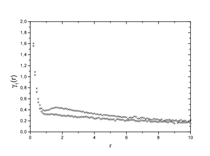
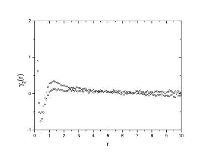
FIG. 3.: The skewness (a) and the curtosis (b) of the traveling salesman problem (crosses) compared to those of the rank $2$ daisy model (diamonds).

FIG. 4.: Fig. 4: Nearest-neighbour spacing distribution for the traveling salesman problem (dashed line) compared to that of the rank $2$ daisy model (full lines)

Summarizing, we have shown that semi-Poisson statistics can be obtained from a very simple model without any dynamical implications. This model actually pertains to a family of models that seem to be relevant in situations where the usual banded matrix models and the Porter Rosenzweig model are grossly inadequate. We obtain this family by retaining every $(r+1)$th level of a random sequence. A similar selection process could be performed for the classical ensembles of Cartan (e.g. the GOE)[12]. Whether this leads to useful results beyond the two cases mentioned above is an open question.

Acknowledgments

We would like to thank F. Leyvraz for helpful discussions. This project has been supported by DGEP, DGAPA IN-112998, UNAM and CONACYT 25192-E.

REFERENCES

- [1] C.E Porter and N. Rosenzweig, Ann. Acad. Sci. Fenn. 6A, no. 44 (reprinted in C.E. Porter, editor, Statistical Theories of Spectra: Fluctuations ( Academic, New York, 1965 )).
- [2] F. Leyvraz and T.H. Seligman, J. Phys A 23, 1555 (1990).
- [3] T.H. Seligman, J.J.V. Verbaarschot and M. Zirnbauer, Phys. Rev. Lett. 53, 215 (1984); T.H. Seligman, J.J.V. Verbaarschot and M. Zirnbauer, J. Phys A 18, 2751 (1985).
- [4] F.M. Izrailev, Phys. Rep. 196, 299 (1990).
- [5] M.V. Berry and M. Robnik, J. Phys. A: Math Gen 17, 2413 (1984).
- [6] T.H. Seligman and J.J.V. Verbaarshot, J. Phys. A, 18, 2227 (1985).
- [7] B.I. Shklovskii, B. Shapiro, B.R. Sears, P. Lambrianides and H.B. Shore, Phys. Rev. B 47, 11487 (1993).
- [8] E.B. Bogomolny, U. Gerland, and C. Schmit, Phys. Rev. E 59, R1315 (1999).
- [9] U. Gerland, Ph. D. Thesis Quantum Chaos and Disordered Systems: How close is the analogy?, University of Heidelberg, Germany (1998).
- [10] R.A. Méndez, A. Valladares, J.Flores, T.H. Seligman and O. Bohigas, Physica A 232, 554 (1996).
- [11] D. Chowdhury, Spin Glasses and other frustrated systems, (World Scientific, Singapore, 1986). p. 251
- [12] E. Cartan, Abh. Math. Sem. Univ. Hamburg 11 , 116 (1935); L.K. Hua, Harmonic analysis of functions of several complex variables in the classical domains, (AMS, Providence, 1963).