Disentangling Scaling Properties in Anisotropic and Inhomogeneous Turbulence.

Abstract

We address scaling in inhomogeneous and anisotropic turbulent flows by decomposing structure functions into their irreducible representation of the SO(3) symmetry group which are designated by $j,m$ indices. Employing simulations of channel flows with Re${}_{\lambda}\approx 70$ we demonstrate that different components characterized by different $j$ display different scaling exponents, but for a given $j$ these remain the same at different distances from the wall. The $j=0$ exponent agrees extremely well with high Re measurements of the scaling exponents, demonstrating the vitality of the SO(3) decomposition.

Version of

Most of the available data analysis and theoretical thinking about the universal statistics of the small scale structure of turbulence assume the existence of an idealized model of homogeneous and isotropic flow. In fact most realistic flows are neither homogeneous nor isotropic. Accordingly, one can analyze the data pertaining to such flows in two ways. The traditional one has been to disregard the inhomogeneity and anisotropy, and proceed with the data analysis assuming that the results pertain to the homogeneous and isotropic flow. The second, which is advocated in this Letter, is to take the anisotropy explicitly into account, to carefully decompose the relevant statistical objects into their isotropic and anisotropic contributions, and assess the degree of universality of each component separately. We analyze here direct numerical simulations of a channel flow with Re${}_{\lambda}\approx 70$ [1, 2, 3]. The main conclusion of this Letter is that this procedure is unavoidable; in particular it highlights the universality of the scaling exponents of the isotropic sector which are presumably those governing the universal small scale statistics at very high Reynolds numbers. In agreement with recent studies of the this subject [4, 5]we report that different irreducible representations of the symmetry group (characterized by indices $j,m$) exhibit scalar functions that scale with apparently universal exponents that differ for different $j$. The exponents found at low values of the Reynolds number for the $j=0$ (isotropic) sector are in excellent agreement with high Re results; these exponents are invariant to the position in the inhomogeneous flow, leading to reinterpretation of recent findings of position dependence as resulting from the intervention of the anisotropic sectors. The latter have nonuniversal weights that depend on the position in the flow.

We consider here channel flow simulations on a grid of $256$ points in the stream-wise direction $\hat{x}$, and $(128\times 128)$ in the other two directions, $\hat{y},\hat{z}$. We denote by $\hat{z}$ the direction perpendicular to the walls and by $\hat{y}$ the span-wise direction in planes parallel to the walls. We employ periodic boundary conditions in the span-wise and stream-wise directions and no-slip boundary conditions on the walls. The Reynolds number based on the Taylor scale is $Re_{\lambda}\approx 70$ in the center of the channel $(z=64)$. The simulation is fully symmetric with respect to the central plane. The flow correctly develops a mean profile in the stream-wise direction which depends only on the distance from the wall, $U_{x}(z)$. The mean profile shows the three typical regimes: a laminar linear mean profile inside the viscous sublayers, a logarithmic profile for intermediate distances and finally a parabolic mean profile in the core of the channel. For more details on the averaged quantities and on the numerical code the reader is referred to [1, 3].

Previous analysis of the same data-base [1] as well as of other DNS [6] and experimental data [7, 8] in anisotropic flows found that the scaling properties of energy spectra, energy co-spectra and of longitudinal structure functions exhibit strong dependence on the local degree of anisotropy. For example, in [2] the authors studied the longitudinal structure functions at fixed distances from the walls:

$$S^{(p)}(R,z)\equiv<(v_{x}(x+R,y,z)-v_{x}(x,y,z))^{p}>_{z}$$

where $<\cdots>_{z}$ denotes a spatial average on a plane at a fixed height $z$, $1<z<64$. For this set of observables they found that: (i) These structure functions did not exhibit clear scaling behavior as a function of the distance $R$. Consequently, one needed to resort to Extended-Self-Similarity (ESS) [9] in order to extract a set of relative scaling exponents $\hat{\zeta^{z}}(p)\equiv\zeta^{z}(p)/\zeta^{z}(3)$; (ii) the relative exponents, $\hat{\zeta^{z}}(p)$ depended strongly on the height $z$. Moreover, only at the center of the channel and very close to the walls the error bars on the relative scaling exponents extracted by using ESS were small enough to claim the very existence of scaling behavior in any sense. Similarly, an experimental analysis of a turbulent flow behind a cylinder [7] showed a strong dependence of the relative scaling exponents on the position behind the cylinder for not too big distances from the obstacle, i.e. where anisotropic effects may still be relevant in a wide range of scales. In the following we present an interpretation of the variations in the scaling exponents observed in non-isotropic and non-homogeneous flows upon changing the position in which the analysis is performed. In particular, we will show that decomposing the statistical objects into their different $(j,m)$ sectors rationalizes the findings, i.e. scaling exponents in given $(j,m)$ sector appear quite independent of the spatial location; only the amplitudes of the SO(3) decomposition depend strongly on the spatial location. These findings, if confirmed by other independent measurements, would suggest that the apparent dependence of scaling exponents for longitudinal structure functions on the location in a non-homogeneous flow results from of a superposition of power laws each of which is characterized by its own universal scaling exponent. The amplitudes of the various contributions may depend on the local degree of anisotropy and non-homogeneity.

Our method of analysis is quite simple [4, 5]. We start by a direct measurement of the longitudinal structure functions

$$S^{(p)}({\mathchoice{{\hbox{\boldmath$\displaystyle r$}}}{{\hbox{\boldmath$\textstyle r$}}}{{\hbox{\boldmath$\scriptstyle r$}}}{{\hbox{\boldmath$\scriptscriptstyle r$}}}}^{c},{\mathchoice{{\hbox{\boldmath$\displaystyle R$}}}{{\hbox{\boldmath$\textstyle R$}}}{{\hbox{\boldmath$\scriptstyle R$}}}{{\hbox{\boldmath$\scriptscriptstyle R$}}}})=\left<\left[\left({\mathchoice{{\hbox{\boldmath$\displaystyle u$}}}{{\hbox{\boldmath$\textstyle u$}}}{{\hbox{\boldmath$\scriptstyle u$}}}{{\hbox{\boldmath$\scriptscriptstyle u$}}}}({{\mathchoice{{\hbox{\boldmath$\displaystyle r$}}}{{\hbox{\boldmath$\textstyle r$}}}{{\hbox{\boldmath$\scriptstyle r$}}}{{\hbox{\boldmath$\scriptscriptstyle r$}}}}^{c}+{\mathchoice{{\hbox{\boldmath$\displaystyle R$}}}{{\hbox{\boldmath$\textstyle R$}}}{{\hbox{\boldmath$\scriptstyle R$}}}{{\hbox{\boldmath$\scriptscriptstyle R$}}}}})-{\mathchoice{{\hbox{\boldmath$\displaystyle u$}}}{{\hbox{\boldmath$\textstyle u$}}}{{\hbox{\boldmath$\scriptstyle u$}}}{{\hbox{\boldmath$\scriptscriptstyle u$}}}}({{\mathchoice{{\hbox{\boldmath$\displaystyle r$}}}{{\hbox{\boldmath$\textstyle r$}}}{{\hbox{\boldmath$\scriptstyle r$}}}{{\hbox{\boldmath$\scriptscriptstyle r$}}}}^{c}-{\mathchoice{{\hbox{\boldmath$\displaystyle R$}}}{{\hbox{\boldmath$\textstyle R$}}}{{\hbox{\boldmath$\scriptstyle R$}}}{{\hbox{\boldmath$\scriptscriptstyle R$}}}}})\right)\cdot\hat{\mathchoice{{\hbox{\boldmath$\displaystyle R$}}}{{\hbox{\boldmath$\textstyle R$}}}{{\hbox{\boldmath$\scriptstyle R$}}}{{\hbox{\boldmath$\scriptscriptstyle R$}}}}\right]^{p}\right>$$ (1)

Note that the two velocity fields are measured at the extremes of the diameter of a sphere of radius $R$ centered at ${\mathchoice{{\hbox{\boldmath$\displaystyle r$}}}{{\hbox{\boldmath$\textstyle r$}}}{{\hbox{\boldmath$\scriptstyle r$}}}{{\hbox{\boldmath$\scriptscriptstyle r$}}}}^{c}$. Due to the inhomogeneity this function depends explicitly on ${\mathchoice{{\hbox{\boldmath$\displaystyle r$}}}{{\hbox{\boldmath$\textstyle r$}}}{{\hbox{\boldmath$\scriptstyle r$}}}{{\hbox{\boldmath$\scriptscriptstyle r$}}}}^{c}$. Due to the anisotropy the function depends on the orientation of the separation vector $2{\mathchoice{{\hbox{\boldmath$\displaystyle R$}}}{{\hbox{\boldmath$\textstyle R$}}}{{\hbox{\boldmath$\scriptstyle R$}}}{{\hbox{\boldmath$\scriptscriptstyle R$}}}}$ as well as on its magnitude. The average must be taken over different time frames. Typically we have used 160 time frames for such an average. The time frames are separated by about one eddy turn over time. In each time frame we also improved the statistics by averaging over one fourth of the total number of spatial points in the plane at fixed $z$, invoking the homogeneity in the span-wise and stream-wise directions, $\hat{x},\hat{y}$. Thus we have finally about $1\times 10^{6}$ contributions to each average.

Having computed $S^{(p)}({\mathchoice{{\hbox{\boldmath$\displaystyle r$}}}{{\hbox{\boldmath$\textstyle r$}}}{{\hbox{\boldmath$\scriptstyle r$}}}{{\hbox{\boldmath$\scriptscriptstyle r$}}}}^{c},{\mathchoice{{\hbox{\boldmath$\displaystyle R$}}}{{\hbox{\boldmath$\textstyle R$}}}{{\hbox{\boldmath$\scriptstyle R$}}}{{\hbox{\boldmath$\scriptscriptstyle R$}}}})$ we decompose it into the irreducible representations of the SO(3) symmetry group according to:

$$S^{(p)}({\mathchoice{{\hbox{\boldmath$\displaystyle r$}}}{{\hbox{\boldmath$\textstyle r$}}}{{\hbox{\boldmath$\scriptstyle r$}}}{{\hbox{\boldmath$\scriptscriptstyle r$}}}}^{c},{\mathchoice{{\hbox{\boldmath$\displaystyle R$}}}{{\hbox{\boldmath$\textstyle R$}}}{{\hbox{\boldmath$\scriptstyle R$}}}{{\hbox{\boldmath$\scriptscriptstyle R$}}}})=\sum_{j,m}S^{(p)}_{j,m}({\mathchoice{{\hbox{\boldmath$\displaystyle r$}}}{{\hbox{\boldmath$\textstyle r$}}}{{\hbox{\boldmath$\scriptstyle r$}}}{{\hbox{\boldmath$\scriptscriptstyle r$}}}}^{c},|{\mathchoice{{\hbox{\boldmath$\displaystyle R$}}}{{\hbox{\boldmath$\textstyle R$}}}{{\hbox{\boldmath$\scriptstyle R$}}}{{\hbox{\boldmath$\scriptscriptstyle R$}}}}|)Y_{j,m}(\hat{\mathchoice{{\hbox{\boldmath$\displaystyle R$}}}{{\hbox{\boldmath$\textstyle R$}}}{{\hbox{\boldmath$\scriptstyle R$}}}{{\hbox{\boldmath$\scriptscriptstyle R$}}}})\ .$$ (2)

We expect that when scaling behavior sets in (presumably at high enough Re) we should find:

$$S^{(p)}_{j,m}({\mathchoice{{\hbox{\boldmath$\displaystyle r$}}}{{\hbox{\boldmath$\textstyle r$}}}{{\hbox{\boldmath$\scriptstyle r$}}}{{\hbox{\boldmath$\scriptscriptstyle r$}}}}^{c},|{\mathchoice{{\hbox{\boldmath$\displaystyle R$}}}{{\hbox{\boldmath$\textstyle R$}}}{{\hbox{\boldmath$\scriptstyle R$}}}{{\hbox{\boldmath$\scriptscriptstyle R$}}}}|)\sim a_{j,m}({\mathchoice{{\hbox{\boldmath$\displaystyle r$}}}{{\hbox{\boldmath$\textstyle r$}}}{{\hbox{\boldmath$\scriptstyle r$}}}{{\hbox{\boldmath$\scriptscriptstyle r$}}}}^{c})|R|^{\zeta_{j}(p)}\ .$$ (3)

In other words, we expect [4] the scaling exponent $\zeta^{j}(p)$ to be independent of $m$.

The first result that we want to display is that by applying the SO(3) decomposition we seem to improve significantly the very existence of scaling behavior. In Fig.1 we show (i) the log-log plot of the raw structure function (1) with $p=4$ measured on the central plane with the vector ${\bf R}$ in the streamwise direction, ${\bf R}=R\hat{x}$, and (ii) the fully isotropic sector $S^{(4)}_{0,0}({\mathchoice{{\hbox{\boldmath$\displaystyle r$}}}{{\hbox{\boldmath$\textstyle r$}}}{{\hbox{\boldmath$\scriptstyle r$}}}{{\hbox{\boldmath$\scriptscriptstyle r$}}}}^{c},|{\mathchoice{{\hbox{\boldmath$\displaystyle R$}}}{{\hbox{\boldmath$\textstyle R$}}}{{\hbox{\boldmath$\scriptstyle R$}}}{{\hbox{\boldmath$\scriptscriptstyle R$}}}}|)$ with the average in (1) taken on the sphere centered on the central plane $r^{c}_{z}=64$.

FIG. 1.: Log-log plot of the isotropic sector of the 4th order structure function $S^{(4)}_{0,0}$, vs. $R$ at the center of the channel $r^{c}_{z}=64$ (+). The data represented by ($\times$) correspond to the raw longitudinal structure function, $S^{(4)}(r^{c}_{z}=64,R\hat{x})$ averaged over the central plane only. The dashed line corresponds to the intermittent isotropic high-Reynolds numbers exponents $\zeta(4)=1.28$.

It appears that already at this fairly low Reynolds number the $j=0$ sector shows decent scaling behavior as a function of $R$. This is in marked contrast with the raw structure function for which no scaling behavior is detectable ($\times$ symbols in Fig.1). For the raw quantity the method of “extended-self-similarity” (ESS) [9] is unavoidable if one wants to extract any kind of apparent scaling exponent. In our analysis we found similar results also for higher order structure functions. The scaling behavior is improved dramatically for the components and it can be seen even without ESS. Nevertheless we will use ESS below for quantitative reading of the exponents within every sector.

The second point we would like to stress is the apparent invariance of the scaling exponents belonging to the same $(j,m)$ sector with respect to changing the spatial location in the flow. To study this issue quantitatively we resort to ESS, and examine the relative scaling of, say, structure functions of order $n$ with respect to the structure function of order $2$ for $n=3,4...$. The ESS method is applied in each $(j,m)$ sector separately.

In Fig.2 we show two typical ESS plots for longitudinal structure functions of order 4 vs longitudinal structure functions of order 2 both at the center $z=64$ and at $z=32$ in the sector $j=0$. Also, in the inset the quality of the scaling can be appreciated by looking at the logarithmic local slopes of $\log(S^{(4)}_{0,0}({\bf r^{c}},|R|))$ vs $\log(S^{(2)}_{0,0}({\bf r^{c}},|R|))$ as a function of $R$ for the same two different central position of the sphere: at the center of the channel ($r^{c}_{z}=64$) and at one quarter of the total channel height ($r^{c}_{z}=32$). The two curves give the same global relative scaling exponent. The best fits for the relative scaling exponents in the sector $(j=0)$ give $\hat{\zeta}^{z=64}_{0}(4)\equiv\zeta^{z=64}_{0}(4)/\zeta^{z=64}_{0}(2)=1.84\pm 0.05$ at the center and $\hat{\zeta}^{z=32}_{0}(4)=1.82\pm 0.04$ at $r^{c}_{z}=32$. This result is remarkable and together with the experimental result of ref.[5] it provides strong evidence for the universality of scaling exponent as defined in distinct $(j,m)$ sectors. We recall that the accepted value of this relative exponent in high-Re experiments is $\zeta(4)/\zeta(2)\approx 1.82\pm 0.02$ [10].

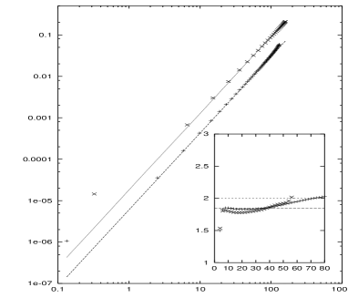
FIG. 2.: Isotropic sector: ESS plot of $\log S^{(4)}_{0,0}$ vs $\log S^{(2)}_{0,0}$ at the center, $r^{c}_{z}=64$, (bottom curve) and at $r^{c}_{z}=31$ (top curve), the straight lines are the best fits with slope $1.82$. Inset: local slope of $\log S^{(4)}_{0,0}$, vs. $\log S^{(2)}_{0,0}$ as a function of $R$, for two different location in the channel: ($+$) center of the channel $r_{z}^{c}=64$, ($\times$) one quarter of the total height $r_{z}^{c}=32$. The local slopes are very close. For comparison we have also plotted a horizontal curve corresponding to the accepted anomalous high-Reynolds number value, $\zeta(4)/\zeta(2)=1.82$.

Similarly, but affected from larger error bars, one recovers the same invariance with respect to higher order moments. For instance we measure $\hat{\zeta}^{z=64}_{0}(6)\sim\hat{\zeta}^{z=32}_{0}(6)=2.5\pm 0.1$. As for relative scaling exponents of higher $j$ sectors, the scaling is less clean and therefore we may only quote qualitative estimates. As an example, for relative scaling exponents of the $(j=2,m=2)$ and $(j=2,m=0)$ sectors we have $\hat{\zeta}^{z=64}_{2,0}(4)=1.1\pm 0.1$, $\hat{\zeta}^{z=32}_{2,0}(4)=1.15\pm 0.1$, $\hat{\zeta}^{z=64}_{2,2}(4)=1.3\pm 0.1$, $\hat{\zeta}^{z=32}_{2,2}(4)=1.\pm 0.1$.

To underline the quantitative improvement resulting from the application of the SO(3) decomposition we show in Fig 3 the logarithmic local slopes of the raw structure functions $S^{(4)}(r_{z}^{c},R\hat{x})$ vs. $S^{(2)}(r_{z}^{c},R\hat{x})$ at $r_{z}^{c}=64$ and at $r_{z}^{c}=32$. Also the logarithmic local slopes of the projection on the $j=0$ sector at the same two distances from the walls are presented. As is evident, the raw structure function at the center of the channel and the two $j=0$ projections are is in good agreement with the high-Reynolds numbers estimate $\zeta(4)/\zeta(2)=1.82$ while a clearly spurious departure is seen for the raw structure functions at $r_{c}^{z}=32$.

FIG. 3.: Logarithmic local slopes of the ESS plot of raw structure function of order 4 versus raw structure function of order 2 at $r_{c}^{z}=64$ ($\times$), at $r_{c}^{z}=32$ ($\star$) and of the $j=0$ projection centered at $r_{c}^{z}=64$ ($+$), and at $r_{c}^{z}=32$($\Box$). Also two horizontal lines corresponding to the high-Reynolds number limit, $1.82$, and to the K41 non-intermittent value, $2$, are shown.

Notice that due to the invariance of Eq.(1) under the inversion ${\bf R}\rightarrow-{\bf R}$ all the amplitudes $a_{j,m}$ belonging to sectors with odd $j$ vanish. Similarly, at the center of the channel the symmetry with respect to the center $R_{z}\rightarrow-R_{z}$ forces all the amplitudes of the components with $j+m$ odd to vanish as well. As a consequence, the sector $(j=2,m=1)$ is relevant only when the center of mass is not in the central plane. When $r^{c}_{z}=32$ we recover indeed good scaling behavior also for this sector but with a relative scaling exponent $\hat{\zeta}^{z=31}_{2,1}(p)$ slightly larger then the relative scaling exponents observed for the other $j=2$ sectors. This fact, which seems to violate the supposed foliation in the $j$ index asserted in Eq.(3) is not well understood at the moment and it may be correlated with the presence of large scale coherent structures (hairpin) oriented at $45^{o}$ with respect to the walls observed in all channel flow simulations [11].

Finally, we discuss briefly the determination of the scaling exponents associated with higher $j$ sectors. The scaling exponent $\zeta_{j=2}(2)$ was estimated by a number of authors on the basis of dimensional analysis [12, 13, 14, 15], and the result is $\zeta_{j=2}(2)=4/3$. There is no theoretical knowledge of the actual value of this exponent with intermittency corrections. Our direct analysis for $j=2$ seems to confirm the dimensional expectation, in agreement with the previous experimental [5] finding.

FIG. 4.: Log-log plot of $S^{(2)}_{2,2}$ ($\star$); $S^{(2)}_{2,0}$ ($\times$) as functions of $R$ at $r^{c}_{z}=32$ and of $S^{(2)}_{2,2}$ as a function of $R$ ($+$) at the center, $r^{c}_{z}=64$. The straight line correspond to the expectation of dimensional analysis : $\zeta_{j=2}(2)=4/3$.

In figure 4 we show the log-log plot of $S^{(2)}_{j,m}({\mathchoice{{\hbox{\boldmath$\displaystyle r$}}}{{\hbox{\boldmath$\textstyle r$}}}{{\hbox{\boldmath$\scriptstyle r$}}}{{\hbox{\boldmath$\scriptscriptstyle r$}}}}^{c},|R|)$ vs $|R|$ for $(j=2,m=2)$ at the center of the channel, and for $(j=2,m=2)$ and $(j=2,m=0)$ at $r^{c}_{z}=32$, superimposed with the straight line with slope $4/3$. The agreement is quite good. Considering the relatively low Reynolds numbers and the fact that the projections on the different sectors depend on the non-universal prefactors $a_{j,m}$ in the decomposition (3), we think that together with the experimental result reported in [5] the present finding gives strong support to the view that the scaling exponents in the $j=2$ sector are universal. We are not able yet to offer the similar support to the possibility that all the scaling exponents in the higher $j$ sectors are universal. Such a conclusion calls for additional careful analysis of the scaling of higher order structure functions and higher $j$ sectors. It is outside the scope of this letter, but it is currently under active study.

In summary, we presented three important results that follow from the SO(3) decomposition of the longitudinal structure functions measured in channel flow simulations [1, 3]: these are (i) The scaling behavior is better defined in separated $(j,m)$ sectors. This is in contradistinction with the raw longitudinal structure function which fails to exhibit any scaling at all. (ii) The isotropic $(0,0)$ component of the structure functions exhibits a universal scaling exponent which is invariant to the spatial location in the flow and the distance from the walls. (iii) The $j=2$ component exhibits a scaling exponent which is compatible with the theoretical expectation and is in excellent agreement with the experimental measurement [5], indicating universality.

The picture that emerges is that the higher order sectors are characterized by scaling exponents that are larger than the fundamental exponent in the isotropic sector. If this is so, it may explain the decay of anisotropy at small scales for high Re flows. In the limit Re$\to\infty$ we expect scaling behavior at very small values of $R/L$ with $L$ being the outer scale. At such small scales only the smallest exponent survives, and this is how the alleged universality of the small scales is achieved.

I Acknowledgments

We are strongly indebted to F. Toschi for helping in the set-up of the data-analysis and for a continuous and fruitful collaboration on the subject. LB is partially supported by INFM (PRA-TURBO). IP acknowledges the partial support of the German-Israeli Foundation, The Israel Science Foundation, the European Commission under the Training and Mobility of Researchers program and the Naftali and Anna Backenroth-Bronicki Fund for Research in Chaos and Complexity.

REFERENCES

- [1] G. Amati, R. Benzi and S. Succi, Phys. Rev. E 55 6985 (1997).
- [2] F. Toschi, G. Amati, S. Succi. R. Benzi and R. Piva, “Intermittency of structure functions on channel flow turbulence”, Phys. Rev. Lett. submitted (1998).
- [3] G. Amati, S. Succi and R. Piva, Int. Jour. Mod. Phys. C 8 869 (1997).
- [4] I. Arad, V.S. L’vov and I. Procaccia, Phys. Rev. E, in press.
- [5] I. Arad, B. Dhruva, S. Kurien, V.S. L’vov, I. Procaccia and K.R. Sreenivasan, Phys. Rev. Lett, 81, 5330 (1998)
- [6] V. Borue and S.A. Orszag, J. Fluid. Mech. 306 293 (1996);
- [7] S.G. Saddoughi and S.V. Veeravalli, J. Fluid. Mech. 268 333 (1994).
- [8] E. Gaudin, B. Protas, S. Gouion-Durand, J. Wojciechowski and J.E Wesfried, Phys. Rev. E 57 R9 (1998).
- [9] R. Benzi, S. Ciliberto, R. Tripiccione, C. Baudet, F. Massaioli and S. Succi, Phys. Rev. E 48 R29 (1993).
- [10] R. Benzi, S. Ciliberto, C. Baudet and G.R. Chavarria, Physica D 80 385 (1993).
- [11] J. Kim and P. Moin, J. Fluid. Mech. 162 339 (1986).
- [12] J.L. Lumley, Phys. Fluids 8 1056 (1965).
- [13] V. Yakhot, Phys. Rev. E 49 2887 (1994).
- [14] G. Falkovich and V. S. L’vov, Chaos Solitons and Fractals 5 1855 (1995).
- [15] S. Grossmann, D. Lohse, V. S. L’vov and I. Procaccia, Phys. rev. Lett. 73, 432 (1994)