Defect-freezing and Defect-unbinding in the Vector Complex Ginzburg-Landau Equation.

Abstract

We describe the dynamical behavior found in numerical solutions of the Vector Complex Ginzburg-Landau equation in parameter values where plane waves are stable. Topological defects in the system are responsible for a rich behavior. At low coupling between the vector components, a frozen phase is found, whereas a gas-like phase appears at higher coupling. The transition is a consequence of a defect unbinding phenomena. Entropy functions display a characteristic behavior around the transition.

1 Introduction

Spatially extended nonlinear dynamical systems display an amazing variety of behavior including pattern formation, self-organization, and spatiotemporal chaos[1]. Transition phenomena between different kinds of states share some characteristics with phase transitions in equilibrium systems. Symmetry breaking, topological defects, and Goldstone modes, for instance, are commonly found. Nevertheless, a much larger variety of collective effects are possible in these far-from-equilibrium systems.

In this paper we report some numerical results on the behavior of the Vector Complex Ginzburg-Landau (VCGL) equation [2, 3], a model originally developed in the study of pattern formation in optical systems [4]. It consists of a set of two coupled complex Ginzburg-Landau equations which could be thought as the two components of a vector equation :

$$\partial_{t}A_{\pm}=A_{\pm}+(1+i\alpha)\nabla^{2}A_{\pm}-(1+i\beta)(|A_{\pm}|^{2}+\gamma|A_{\mp}|^{2})A_{\pm}.$$ (1)

The VCGL equation appears naturally in situations where a two-component vector field starts to oscillate after undergoing a Hopf bifurcation. This is the case of the transverse electric vector field in a resonant optical cavity near the onset of laser emission. The two complex fields $A_{\pm}$ are the complex envelopes of the two components (the circularly polarized components in the optical case) of the oscillating field. The parameter $\alpha$ measures dispersion or diffraction effects whereas $\beta$ is a measure of nonlinear frequency renormalization. $\gamma$ is the coupling between the components, so that for $\gamma=0$ one obtains two uncoupled scalar Ginzburg-Landau equations.

The onset of oscillations breaks two continuous symmetries. On the one hand, the phase of the oscillations destroys time translation invariance. On the other the direction of oscillations breaks isotropy by singling out a vector orientation. Typically these symmetries are broken differently in different parts of the system, so that regions in different oscillation states, with topological defects between them, appear and compete.

For the case $\gamma=0$, equivalent to the scalar case, a phase diagram charting the different states at different parameter values has been obtained both in one and in two dimensions [5]. In the general vectorial or coupled case, however, our knowledge is much more partial. Here we will describe states appearing in two spatial dimensions for $\gamma$ real, $0\leq\gamma<1$, and $\alpha$ and $\beta$ such that plane waves $A_{\pm}=Q_{\pm}e^{i(\bf k_{\pm}\cdot\bf x-\omega_{\pm}t)}$ are linearly stable solutions (a necessary condition is $1+\alpha\beta>0$). The range of parameters that we consider is relevant to describe laser emission when atomic properties favor linear polarization in a broad area laser with large detuning between atomic and cavity frequencies.

The following two sections describe our results for the behavior of the system in our range of parameter values. We show the existence of a transition between a frozen phase and a gas-like phase. After the conclusions section, an Appendix gives some details on the numerical algorithm used.

2 Defect-dominated frozen phase

Despite the existence and stability of plane-wave solutions, typical evolution starting from random initial conditions leads to complex evolving states. For $\gamma$ small the state of each component superficially resembles the one obtained for the scalar equation (see Fig. 1): the dominant objects are spiral waves, emanating from or sinking into a defect (a zero of the complex field, giving a phase singularity) core. Despite the similarities, there are important differences between defects in the scalar case and in the present vectorial case. In the scalar case there is only one complex field, so that there is a single phase and thus a single type of charge associated to its singularities or defects. In our case there are two complex fields, $A_{+}$ and $A_{-}$, which can vanish independently, giving rise to two independent charges. The topological charges of a defect are defined by

$$n_{\pm}=\frac{1}{2\pi}\oint_{\Gamma}\vec{\nabla}\phi_{\pm}\cdot d\vec{r}\ ,$$ (2)

where $\Gamma$ is a closed path around the defect, and the phases $\phi_{\pm}$ are defined by the relations $A_{\pm}=|A_{\pm}|e^{i\phi_{\pm}}$. Numerically we do not find in the system the spontaneous emergence of any topological charge with modulus greater than 1 starting from random initial conditions.

It is possible to make a classification of defects using standard topological arguments [6, 7]. We call vectorial defect a defect which is a singularity of both components of the field (i.e. both components vanish at the same point). A vectorial defect is of argument type when the charges of the two field components have the same signs, i.e., when $n_{+}=n_{-}=1$ or $n_{+}=n_{-}=-1$. If the charges are of opposite signs, i.e., when $n_{+}=-n_{-}=1$ or $n_{+}=-n_{-}=-1$, the vectorial defect is of director type. We call mixed defect a defect that is present just in one component of the field.

For $\gamma=0$ there is no interaction between the two fields and thus binding of mixed defects to form vectorial defects would not occur generically. By increasing $\gamma$ we observe that all kinds of defects appear leading to configurations which evolve very slowly in time. Such configurations are representative of a frozen or glassy state. For example, for $\gamma=0.1$, $\alpha=0.2$, $\beta=2$ and large times (Fig. 1), the system evolves into a state in which the fields are organized in domains of nearly constant modulus separated by shocks. There is a vectorial defect at the center of each domain. This defect core emits or receives phase waves which entrain the whole domain. Perturbations and mixed defects are ejected away from the defect core with a group velocity. The mixed defects accumulate at the domain borders. In Fig. 1 we also show the global and relative phases, $\phi_{g}=\phi_{+}+\phi_{-}$ and $\phi_{r}=\phi_{+}-\phi_{-}$. An argument defect has a global phase $\phi_{g}$ that rotates $4\pi$ around the defect core, while the relative phase $\phi_{r}$ rotates 0. For a director defect, $\phi_{g}$ rotates 0 and $\phi_{r}$ rotates $4\pi$. In consequence argument and director defects are easily distinguished in the plot of the global phase: A two-armed spiral is formed around an argument defect, while a target pattern is seen in the domain of a director defect. Mixed defects appear as points around which the global or relative phase rotates by $2\pi$. The modulus of this kind of configuration evolves very slowly in time, so that we could call it a frozen or glassy state.

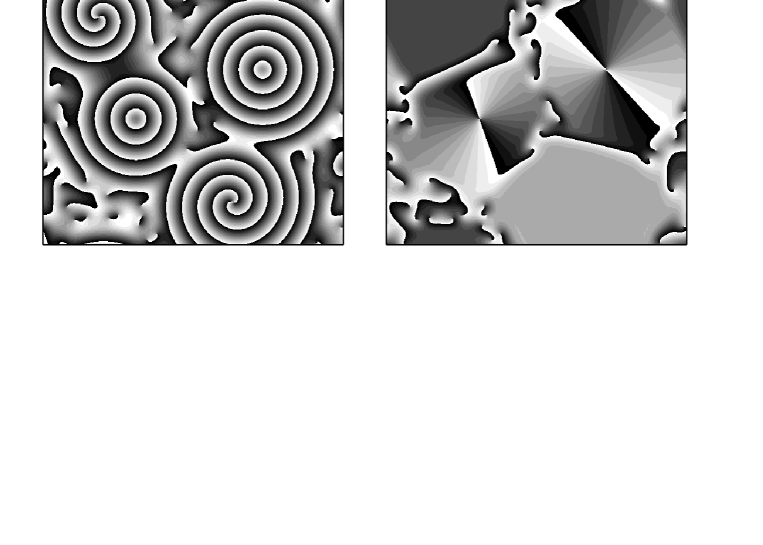
Figure 1: Frozen configurations for $\gamma=0.1$, $\alpha=0.2$ and $\beta=2$, displaying the different kinds of defects. (a) $|A_{+}|^{2}$, (b) $|A_{-}|^{2}$, (c) global phase $\phi_{g}$, and (d) relative phase $\phi_{r}$. In the modulus plots, black points are zeros of the corresponding field and white points locate the maximum values

As $\gamma$ increases the structure of the mixed defects becomes such that a maximum in the modulus of one of the components appears where the other component presents a singularity (see Fig. 2). Such anticorrelation, which also occurs for the shocks separating the regions dominated by a vectorial defect, becomes more evident by further increasing $\gamma$. This feature is also present in the one-dimensional case[8]: no topological defects exist in $d=1$, but a spatially localized minimum of one field, which moves in time, goes together with a maximum of the other field.

3 Unbinding transition to a gas phase

There is a critical value ($\gamma\approx 0.35$ for $\alpha=0.2$, $\beta=2$, as in Figs.  1 and 2) above which vectorial defects disappear. We observe two different annihilation processes: a) One of the two singularities that form the vectorial defect is annihilated in the collision with a mixed defect, in the same component but of opposite charge, which migrates from the boundaries of a domain. A mixed defect, with charge associated to the other component, is thus left in the system. b) The vectorial defect splits into two spatially separated mixed defects, one in each component.

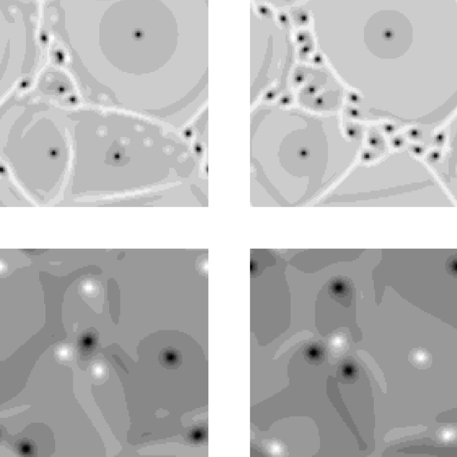
Figure 2: Field configurations for $\alpha=0.2$, and $\beta=2$. Gray code as in Fig. 1. Top: $\gamma=0.2$; wave domains dominated by vectorial defect cores are still present. Maxima in the modulus of one component are clearly associated with mixed defects in the other. Bottom: $\gamma=0.8$; defect unbinding has occurred and only mixed defects, with associated maxima in the non-singular component, are present. First column: $|A_{+}|^{2}$, second column: $|A_{-}|^{2}$.

When the vectorial defects disappear, spiral-wave domains dissolve and the frozen structure transforms into a mobile configuration with fast active dynamics. Fig. 2 (bottom) shows a typical snapshot: mixed defects travel freely around the system as in a kind of “gas phase”. The anticorrelation between the two components is quite evident at this large value of $\gamma$. The transition between the frozen and the gas behavior is rather sharp, and can be thought as a kind of vortex unbinding.

One way of characterizing the different kinds of behavior and transitions between them is by means of an entropy measure $H(X)=-\sum_{x}p(x)\ln p(x)$, where $p(x)$ is the probability that $X$ takes the value $x$. $H(X)$ measures the randomness of a discrete variable $X$. We can compute the single-point entropies of the modulus of the field components by considering the discretized values of $|A_{+}|$ and $|A_{-}|$ as random variables ($X=|A_{+}|$ or $|A_{-}|$; we discretize the range of these variables into 200 values). The associated probability distributions are defined from the ensemble of values collected from different space-time points. In Fig. 3 we plot the entropy of $|A_{+}|$ and $|A_{-}|$ as functions of $\gamma$. For low values of $\gamma$ the system is in the frozen state consisting in large domains of uniform modulus surrounding vectorial defects. These domains impose some degree of order which gives low values to the entropies. For $\gamma=0.25$ the size of the domains diminishes, and the system becomes more disordered as indicated by the increase of the entropies. There is a maximum of the entropies at $\gamma\simeq 0.3$, which is the value at which the argument defects are seen to annihilate. Thus the maximum in the entropies is signaling the transition from the frozen structure to the gas-like phase. For $\gamma\simeq 0.35$ the director vectorial defects disappear also, so that for higher values of $\gamma$ there are only mixed defects. When $\gamma$ leaves the transition region, the entropies initially decrease, but they increase later with growing $\gamma$ in correspondence with the increasing dynamic disorder in the fields. This behavior of the entropies is in contrast with the one-dimensional case [8], where topological defects are absent. There, entropies maintain an essentially constant value when $\gamma$ varies. The presence of defects in the two-dimensional case is responsible for the distinct behavior of the entropies.

Figure 3: Entropy of $|A_{+}|$ (squares) and $|A_{-}|$ (triangles) as functions of $\gamma$ ($\alpha=0.2$, $\beta=2$).

4 Conclusions

In this Paper we have described qualitatively some aspects of the dynamics of the VCGL equation, focusing in a particular parameter regime of relevance in optics. The presence of different kinds of defects is the characteristic phenomenon organizing other features of the dynamics. Two main “phases”, a frozen or glassy state and a more dynamic gas-like phase, have been identified. The transition between these two phases originates in the unbinding of vectorial defects.

Appendix A Numerical Integration Scheme

The time evolution of the complex fields $A_{\pm}(x,t)$ subjected to periodic boundary conditions is obtained numerically from the integration of the VCGL in Fourier space. The method is pseudospectral and second-order accurate in time. It is the straightforward generalization to two dimensions and two components of the algorithm described in [9] for the scalar Ginzburg-Landau equation. Each Fourier mode $A_{\pm}^{q}$ evolves according to:

$$\partial_{t}A_{\pm}^{q}(t)=-\alpha_{q}A_{\pm}^{q}(t)+\Phi_{\pm}^{q}(t)\>,$$ (3)

where $\alpha_{q}$ is $(1+ic_{1})q^{2}-1$, and $\Phi_{\pm}^{q}$ are the $q$-modes of the non-linear terms in the VCGL equation.

When a large number of modes $q$ is used, the linear time scales $\alpha_{q}$ can take a wide range of values. A way of circumventing this stiffness problem is to treat exactly the linear terms by using the formal solution:

$$A_{\pm}^{q}(t)=e^{-\alpha_{q}t}\left(A_{\pm}^{q}(t_{0})e^{\alpha_{q}t_{0}}+\int_{t_{0}}^{t}\Phi_{\pm}^{q}(s)e^{\alpha_{q}s}ds\right)\>.$$ (4)

From here the following relationship can be obtained:

$$A_{\pm}^{q}(n+1)=e^{-2\alpha_{q}\delta t}A_{\pm}^{q}(n-1)+\frac{1-e^{-2\alpha_{q}\delta t}}{\alpha_{q}}\Phi_{\pm}^{q}(n)+{\cal O}(\delta t^{3})\>.$$ (5)

Expressions of the type $f(n)$ are shortcuts for $f(t=n\delta t)$. Scheme (5) alone is unstable for the VCGL equation. To fix this one can derive the auxiliary expression

$$A_{\pm}^{q}(n)=e^{-\alpha_{q}\delta t}A_{\pm}^{q}(n-1)+\frac{1-e^{-\alpha_{q}\delta t}}{\alpha_{q}}\Phi_{\pm}^{q}(n-1)+{\cal O}(\delta t^{2})\>,$$ (6)

and the algorithm proceeds as follows:

1. Starting from $A_{\pm}^{q}(n-1)$ and Fourier inverting to get $A_{\pm}(\bf x,n-1)$ one can calculate the nonlinear terms in direct space and then obtain $\Phi_{\pm}^{q}(n-1)$.

2. Eq. (6) is used to obtain an approximation to $A_{\pm}^{q}(n)$.

3. The non-linear terms $\Phi_{\pm}^{q}(n)$ are now calculated from these $A_{\pm}^{q}(n)$ by going to real space as before.

4. The fields at step $n+1$ are calculated from (5) by using $A_{\pm}^{q}(n-1)$ and $\Phi_{\pm}^{q}(n)$.

At each iteration, we get $A_{q}(n+1)$ from $A_{q}(n-1)$, and the time advances by $2\delta t$.

The number of Fourier modes depends on the space discretization. We have used $dx=1$ in lattices of size $128\times 128$ or $256\times 256$. The time step was usually $dt=2\delta t=0.05$.

References

- [*] Web site: http://www.imedea.uib.es/PhysDept/
- [1] M. Cross and P. Hohenberg, Rev. Mod. Phys. 65, 851 (1993).
- [2] M. San Miguel, Phys. Rev. Lett. 75, 425 (1995).
- [3] L. Gil, Phys. Rev. Lett. 70, 162 (1993).
- [4] Lugiato et al. Eds., Chaos, solitons and fractals 70,1251 (1994).
- [5] H. Chaté, in Spatio-Temporal Patterns in Non-equilibrium Complex Systems, Cladis, P.E.& Palffy-Muhoray, P., editors (Addison-Wesley, Reading, 1994); H. Chaté, P. Manneville, Physica A 224, 348-368 (1996).
- [6] L. M. Pismen, Phys. D 73, 244 (1994).
- [7] M. Hoyuelos, P. Colet, E. Hernández-García, and M. San Miguel, to appear (1998).
- [8] A. Amengual, E. Hernández-García, R. Montagne and M. San Miguel, Phys. Rev. Lett. 78, 4379 (1997).
- [9] R. Montagne, E. Hernández-García, A. Amengual, and M. San Miguel, Phys. Rev. E 56, 151 (1997).