Chaotic Dynamics in Iterated Map Neural Networks with Piecewise Linear Activation Function

Abstract

The paper examines the discrete-time dynamics of neuron models (of excitatory and inhibitory types) with piecewise linear activation functions, which are connected in a network. The properties of a pair of neurons (one excitatory and the other inhibitory) connected with each other, is studied in detail. Even such a simple system shows a rich variety of behavior, including high-period oscillations and chaos. Border-collision bifurcations and multifractal fragmentation of the phase space is also observed for a range of parameter values. Extension of the model to a larger number of neurons is suggested under certain restrictive assumptions, which makes the resultant network dynamics effectively one-dimensional. Possible applications of the network for information processing are outlined. These include using the network for auto-association, pattern classification, nonlinear function approximation and periodic sequence generation.

1 Introduction

Since the development of the electronic computer in the 1940s, the serial processing computational paradigm has successfully held sway. It has developed to the point where it is now ubiquitous. However, there are many tasks which are yet to be successfully tackled computationally. A case in point is the multifarious activities that the human brain performs regularly, including pattern recognition, associative recall, etc. which is extremely difficult, if not impossible to do using traditional computation.

This problem has led to the development of non-standard techniques to tackle situations at which biological information processing systems excel. One of the more successful of such developments aims at “reverse-engineering” the biological apparatus itself to find out why and how it works. The field of neural network models has grown up on the premise that the massively parallel distributed processing and connectionist structure observed in the brain is the key behind its superior performance. By implementing these features in the design of a new class of architectures and algorithms, it is hoped that machines will approach human-like ability in handling real-world situations.

Extremely simplified models of neurons connected in a network via suitable connection weights were known to implement various logical functions since the 1940s. The subject received fresh impetus a decade and half ago due to some breakthroughs. These were however restricted to networks subject to convergent dynamics. Such systems tend to a time-independent solution (a “fixed-point” attractor) after starting off from some initial condition. On the other hand, the brain never settles down to a steady state but appears to exhibit a rich variety of non-periodic behavior.

The development of nonlinear dynamical systems theory - in particular, the discovery of “deterministic chaos” in extremely simple systems - has furnished the theoretical tools necessary for analyzing non-convergent network dynamics. Several neurobiological studies have in fact indicated the presence of chaotic dynamics in the brain [1] and its possible role in biological information processing. Thus, the ability to design networks with aperiodic behavior promises to add a new dimension to our understanding of how the brain works.

Several efforts in designing and applying chaotic neural networks have already appeared [2] - [8]. (For further references see [4]). In the present work, a particularly simple model whose state is updated after discrete time intervals is studied. The piecewise linear nature of the model neuron used, not only makes detailed theoretical analysis possible, but also enables an intuitive understanding of the dynamics, at least for a small number of connected elements. This makes it easier to extrapolate to larger networks and suggest possible applications. The proposed model is also particularly suitable for hardware implementation using operational amplifiers (owing to their piecewise linear characteristics).

The rest of the paper is organized as follows. The basic features of the piecewise linear neural model used is described in section 2, along with the biological motivation for such a model. The next section is devoted to analyzing the dynamics of a pair of excitatory and inhibitory neurons, with self- and inter-connections. This simple system shows a wide range of behavior including periodic oscillations, chaos and border-collision bifurcations [9]. Section 4 extends the model to larger networks under certain restrictive conditions. This is followed by a discussion of the possible application of the model to various information processing tasks, such as associative memory and nonlinear function approximation. The rich dynamics of the system allows it to respond to specific inputs with periodic or aperiodic responses (in contrast to a time-independent constant output, as in convergent networks) and also to act as a central pattern generator. We conclude with a short discussion on possible directions for further studies.

2 Piecewise Linear Neuron

Let $u_{n}$ denote the activation state of a model neuron at the $n-$th time interval. If $u_{n}=1$, the neuron is considered to be active (firing), and if $u_{n}=0$, it is quiescent. Then, if $v_{n}$ is the input to the neuron at the $n$th instant, the discrete-time neural dynamics is described by the equation

$$u_{n}={\cal F}(v_{n}),$$ (1)

assuming there to be no effects of delay. The input $v_{n}$ is the weighted sum of the activation states at the $(n-1)$-th instant of all other neurons connected to the neuron under consideration, together with external stimulus (if any). The form of ${\cal F}$ is decided by the input-output behavior of the neuron. Usually, it is taken to be the Heaviside step function, i.e.,

$$\begin{array}[]{lll}{\cal F}(z)&=&1,~{}~{}{\rm if}~{}~{}z>~{}\mu,\\ &=&0,~{}~{}{\rm otherwise},\end{array}$$ (2)

where $\mu$ is known as the threshold.

If the mean firing rate, i.e., the activation state averaged over a time interval, is taken as the dynamical variable, then a continuous state space is available to the system. If $X_{n}$ be the mean firing rate at the $n-$th time interval, then

$$X_{n+1}~{}=~{}F_{\mu}(\Sigma_{j}W_{j}X^{j}_{n}+I_{n}).$$ (3)

Here, $F$ is known as the activation function and $\mu$ is the parameter associated with it. The first term of the argument represents the weighted sum of inputs from all neurons connected with the one under study. $W_{j}$ is the weightage for the connection to the $j$th neuron. $I_{n}$ represents the external stimulus at the $n$th instant.

Considering the detailed biology, there are two transforms occurring at the threshold element. At the input end, the impulse frequency coded information is transformed into the amplitude modulation of the neural current. For single neurons, this pulse-wave transfer function is linear over a small region, with nonlinear saturation at both extremities. At the output end, the current amplitude is converted back to impulse frequency. The wave-pulse transfer-function for single neurons is zero below a threshold, then rises linearly upto a maximum value. Beyond this maximum, the output falls to zero due to “cathodal block”. These relations are time-dependent. For example, the slope of the wave-pulse transfer function decreases with time when subjected to sustained activation (“adaptation”) [1].

The net transformation of a input by a neuron is therefore given by the combined action of the two transfer-functions. Let us approximate the nonlinear pulse-wave transfer function $F_{1}$ with a piecewise linear function, such that

$$\begin{array}[]{lll}F_{1}(z)&=&-c,~{}~{}{\rm if}~{}~{}z<~{}-c/m,\\ &=&m~{}z,~{}~{}{\rm if}~{}~{}-c/m~{}\leq z\leq~{}1/m,\\ &=&1,~{}~{}{\rm if}~{}~{}z>~{}1/m.\end{array}$$ (4)

The wave-pulse transfer function $F_{2}$ is represented as

$$\begin{array}[]{lll}F_{2}(z)&=&0,~{}~{}{\rm if}~{}~{}z<~{}t,\\ &=&m^{\prime}~{}(z-t),~{}~{}{\rm if}~{}~{}t~{}\leq z\leq~{}t+(1/m^{\prime}),\\ &=&0,~{}~{}{\rm if}~{}~{}z>~{}t+(1/m^{\prime}),\end{array}$$ (5)

where $m,m^{\prime}$ are the slopes of $F_{1},F_{2}$ respectively, $c$ is the inhibitory saturation value and $t$ represents a threshold value.

It is easily seen that the combined effect of the two gives rise to the resultant transfer function, $G$, defined as

$$\begin{array}[]{lll}G(z)&=&0,~{}~{}{\rm if}~{}~{}z<~{}t,\\ &=&m~{}m^{\prime}~{}(z-t),~{}~{}{\rm if}~{}~{}t~{}\leq z\leq~{}t+(1/m),\\ &=&m^{\prime}~{}(1-t),~{}~{}{\rm if}~{}~{}t+(1/m)~{}<z\leq~{}t+(1/m^{\prime}),\\ &=&0,~{}~{}{\rm if}~{}~{}z>~{}t+(1/m^{\prime}).\end{array}$$ (6)

In the present work we will assume that $m^{\prime}~{}(1-t)<<t+(1/m^{\prime})$. This condition ensures that the operating region of the neuron does not go into the “cathodal block” zone. This allows us to work with the following simplified neural activation function (upon rescaling) throughout the rest of the paper:

$$\begin{array}[]{lll}F_{a}(z)&=&0,~{}~{}{\rm if}~{}~{}z<~{}t,\\ &=&a~{}(z-t),~{}~{}{\rm if}~{}~{}t~{}\leq z\leq~{}t+(1/a),\\ &=&1,~{}~{}{\rm if}~{}~{}z>~{}t+(1/a),\end{array}$$ (7)

where $a~{}(>0)$ is called the gain parameter of the function (Fig. 1). For infinite gain ($a\rightarrow\infty$), the activation function reverts to the hard-limiting Heaviside step function.

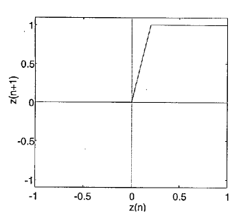
Figure 1: The piecewise linear activation function $F$ for a single neuron (gain parameter, $a$ = 5).

Note that, if neural populations had been considered, instead of single neurons, then sigmoidal activation functions, e.g.,

$$F_{\mu}(z)=1/(1+e^{-\mu z}),$$

would have been the appropriate choice. By varying $\mu$, transfer functions with different slopes would be obtained.

Although, in the present study, the gain parameter, $a$, of the transfer function is considered constant, in general it will be a time-varying function of the activation state, decreasing under constant external stimulation until the neuron goes into a quiescent state. The threshold $t$ is also a dynamic parameter, changing as a result of external stimulation. We have also assumed that the neuron state at the $n$th instant is a function of the state value at the previous instant only. Introducing delay effects into the model, such that,

$$X_{n+1}=F(X_{n},X_{n-1},\ldots,X_{n-\tau}),$$

might lead to novel behavior.

3 Excitatory-Inhibitory Pair Dynamics

Having established the response properties of single neurons, we can now study the dynamics when they are connected. It is observed that, even connecting only an excitatory and an inhibitory neuron with each other leads to a rich variety of behavior, including high period oscillations and chaos. The continuous-time dynamics of pairwise connected excitatory-inhibitory neural populations (with sigmoidal nonlinearity) have been studied before [10]. However, in the present case, the resultant system is updated in discrete-time intervals and the dynamics is governed by piecewise linear mappings. This makes chaotic behavior possible in the proposed neural network model. Chaotic activity has been previously observed in piecewise linear systems, for both continuous-time [11] as well as discrete-time evolution [12] of the system.

If $X$ and $Y$ be the mean firing rates of the excitatory and inhibitory neurons, respectively, then their time evolution is given by the coupled difference equations:

$$X_{n+1}=F_{a}(W_{xx}X_{n}-W_{xy}Y_{n}),$$ (8)

$$Y_{n+1}=F_{b}(W_{yx}X_{n}-W_{yy}Y_{n}).$$

Figure 2: The pair of excitatory ($x$) and inhibitory ($y$) neurons. The arrows and circles represent excitatory and inhibitory synapses, respectively.

The network connections are shown in Fig. 2. Without loss of generality, the connection weightages $W_{xx}$ and $W_{yx}$ can be absorbed into the gain parameters $a$ and $b$ and the correspondingly rescaled remaining connection weightages, $W_{xy}$ and $W_{yy}$, are labeled $k$ and $k^{\prime}$ respectively. For convenience, a transformed set of variables, $Z_{n}=X_{n}-k~{}Y_{n}$ and $Z^{\prime}_{n}=X_{n}-k^{\prime}~{}Y_{n}$, is used. The dynamics is now given by

$$Z_{n+1}=F_{a}(Z_{n})-k~{}F_{b}(Z^{\prime}_{n}),$$ (9)

$$Z^{\prime}_{n+1}=F_{a}(Z_{n})-k^{\prime}~{}F_{b}(Z^{\prime}_{n}).$$

Note that, if $k=k^{\prime}$, the two-dimensional dynamics is reduced to an effective one-dimensional one, simplifying the analysis. We will now examine the cases: $(i)k=k^{\prime}=1$, $(ii)k=k^{\prime}\neq 1$, and $(iii)k\neq k^{\prime}$, in detail. Unless mentioned otherwise, the threshold $t$ will be taken as 0 (a non-zero value of $t$ introduces an affine transformation to $F$).

3.1 $k=k^{\prime}=1$

This represents the condition when the connection weights $W_{xy}=W_{xx}$ and $W_{yy}=W_{yx}$, $(a>b)$. The dynamics is that of an asymmetric tent map (Fig. 3(a)):

$$\begin{array}[]{lll}Z_{n+1}&=&(a~{}-~{}b)~{}Z_{n},~{}~{}{\rm if}~{}~{}0~{}\leq Z_{n}\leq~{}1/a,\\ &=&1~{}-~{}bZ_{n},~{}~{}{\rm if}~{}~{}~{}1/a~{}<Z_{n}\leq~{}1/b,\\ &=&0,~{}~{}{\rm otherwise}.\end{array}$$ (10)

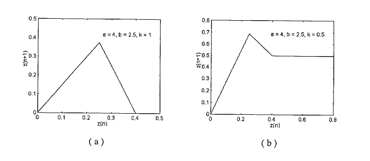
Figure 3: The one-dimensional map representing neural pair dynamics for (a) $k=k^{\prime}=1$ and (b) $k=k^{\prime}\neq 1$.

The fixed points of this system are, $Z^{*}_{1}~{}=~{}0$ and $Z^{*}_{2}~{}=~{}1/(1+b)$. $Z^{*}_{1}$ is stable for $a-b~{}<~{}1$, whereas $Z^{*}_{2}$ exists only when $a-b~{}>~{}1$, and is stable for $b~{}<~{}1$. Beyond this, chaotic behavior is observed unless the maximum output value, i.e., $1-(b/a)$, iterates to the region where $Z>1/b$. The parameter space diagram is shown in Fig. 4.

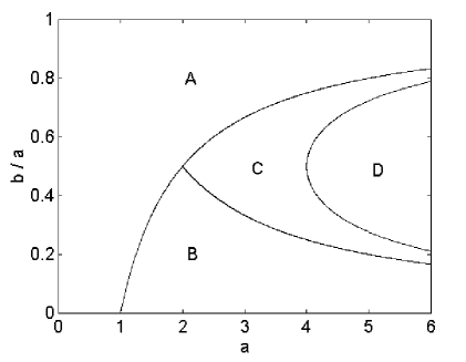
Figure 4: The activation gain $a$ vs. $(b/a)$ parameter space for $k=k^{\prime}=1$. Region A: $z^{*}=0$ stable, B: $z^{*}=1/(1+b)$ stable, C: chaos, D: coexistence of $z^{*}=0$ and a fractal chaotic invariant set.

Along the line $b/a=0.5$, we get the symmetric tent map scenario. So the Lyapunov exponent along this curve grows as $\lambda={\log}_{e}(b)$ for $0<a<4$. This is one of the two special cases where an analytical expression for $\lambda$ can be obtained. The other instance is when the map’s invariant probability distribution, $P(Z)=1$. This occurs when

$$F~{}(1/a)=1-(b/a)=1/b.$$ (11)

Along the curve defined by the above relation, the Lyapunov exponent evolves with the parameter $b/a$ according to

$$\lambda=-b/a~{}{\log}_{e}(b/a)-(1-(b/a)){\log}_{e}(1-(b/a)).$$ (12)

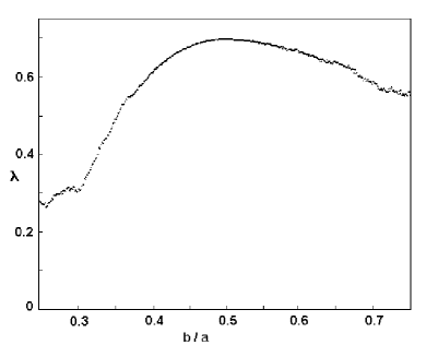
Figure 5: Lyapunov exponent of the chaotic dynamics for $k=k^{\prime}=1$ and $a=4.0$. At $b/a=0.5$, the entire interval $[0,1/b]$ is uniformly visited.

In general, $\lambda$ has to be obtained computationally. Fig. 5 shows $\lambda$ plotted against $b/a$ for $a=4$, when the map is in the chaotic region. A sharp drop to zero is observed in both the terminal points, indicating sharp transition between chaotic and fixed-point behavior at $b/a=0.25$ and 0.75. At $b/a=0.5$, the entire interval $[0,1/b]$ is uniformly visited by the chaotic trajectory ($P(Z)=1$). This corresponds to “fully-developed chaos” in the symmetric tent map for which $\lambda={\log}_{e}(2)\simeq 0.693.$

When $F(1/a)>1/b$, the interval $[0,1/b]$ is divided into a chaotic region of measure zero, defined on a non-uniform Cantor set (in general) and an “escape set” which maps to $Z^{*}_{1}=0$. This is because, for $Z\in(1/b(a-b),(b-1)/b^{2})$, F(Z)=0. Any time an iterate of $Z$ falls in this region, in the next iterate the trajectory will converge to $Z^{*}_{1}$. The points left invariant after one iteration, will be in the two intervals $[0,1/b(a-b)]$ and $[(b-1)/b^{2},1]$. The phase space is thus fragmented into two invariant regions. After $n$ iterations, there will be $2^{n}$ fragments of the chaotic invariant set, with $n!/r!(n-r)!$ ($r=0,1,\ldots,n$) intervals of length $(a-b)^{r}(1-b)^{r-n}$. The fragmentation of the phase space, therefore, has a multifractal nature [13].

The presence of multiple length scales is due to the fact that the slope magnitude of the map is not constant throughout the interval $[0,1/b]$. It is to be noted that, even for $Z$ not belonging to the fractal invariant set, the trajectory might show long chaotic transients until at some iterate it maps to $Z^{*}=0$. For $b/a=0.5$, the map has a constant slope. As a result, the Cantor set is uniform, having exact geometrical self-similarity and a fractal dimension, $D={\log}_{e}(2)/{\log}_{e}(b)$. So, the phase space of the coupled system has a fractal structure in this parameter region, i.e., where $1-(b/a)>1/b$.

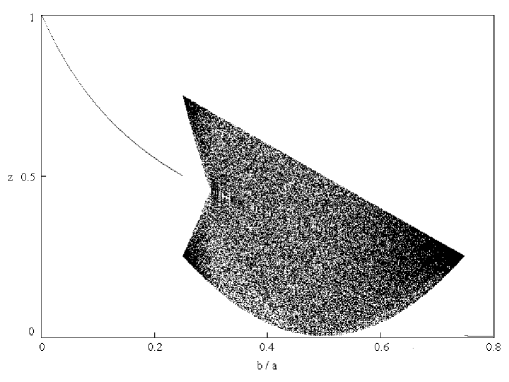
Figure 6: Bifurcation diagram for $k=k^{\prime}=1$ at $a=4.0$.

Fig. 6 shows the bifurcation structure of the map for $a=4$. For $b/a<0.25$, the fixed point $Z^{*}_{2}$ is stable. At $b/a=0.25$ it becomes unstable, leading to bands of chaotic behavior. The chaotic bands collide with the unstable fixed point $Z^{*}_{2}$ at $b/a\simeq 0.2985...$ and merge into a single chaotic band. This band-merging transition is an example of crisis [14] and has been studied in detail for the symmetric tent map [15]. The $b$-value at which the band-merging occurs for a given value of $a$, can be obtained analytically by solving the quartic equation:

$$b^{4}+(1-2a)b^{3}+(a^{2}-a)b^{2}+ab+(a-a^{2})=0.$$ (13)

For $2<a<2.5$, all the roots are complex, implying that band-merging does not occur over this range of $a$-values.

Uniform chaotic behavior occurs at $b/a=0.5$ (the entire interval [0,1/b] is uniformly visited by the chaotic trajectory). The chaotic band collides with the unstable $Z^{*}_{2}$ again at $b/a=0.75$. This boundary crisis destroys chaos and stabilizes the fixed point $Z^{*}_{1}=0$.

3.2 $k=k^{\prime}\neq 1$

This represents the condition when the connection weightages are such that, $W_{xy}/W_{xx}=W_{yy}/W_{yx}=k$, ($a>b$). The dynamics is given by the following map (Fig. 3(b))

$$\begin{array}[]{lll}Z_{n+1}&=&(a~{}-~{}kb)~{}Z_{n},~{}~{}{\rm if}~{}~{}0~{}\leq Z_{n}\leq~{}1/a,\\ &=&1~{}-~{}kbZ_{n},~{}~{}{\rm if}~{}~{}~{}1/a~{}<Z_{n}\leq~{}1/b,\\ &=&1~{}-~{}k,~{}~{}{\rm otherwise}.\end{array}$$ (14)

The key difference with the earlier case is that now the dynamics supports superstable period-$m$ orbits ($m\geq 2$). This is a result of the existence of a region of zero slope ($Z~{}>~{}1/b)$ giving a non-zero output. There are two fixed points of the map, $Z^{*}_{1}=0$ (as before), and,

$$\begin{array}[]{lll}Z^{*}_{2}&=&1-k,~{}{\rm if}~{}0<k<1-(1/b),~{}{\rm or,}\\ &=&1/(1+kb),~{}{\rm if}~{}(a-1)/b>k>1-(1/b).\end{array}$$

$Z^{*}_{2}~{}=~{}1-k$, if it exists, is superstable, as the local slope is zero. On the other hand, $Z^{*}_{2}~{}=~{}1/(1+kb)$ is stable, only if $bk<1$. If the fixed points are unstable, but iterates of $Z$ fall in the region $Z>1/b$, superstable periodic cycles occur. The fixed point, $Z^{*}_{1}~{}=~{}0$, becomes stable when $(a-bk)<1$. Chaotic behavior occurs if none of the fixed points are stable, and no iterate of $Z$ falls in the region $Z>1/b$. The $(b/a)$ vs. $k$ parameter space diagram in Fig. 7 (for $a=4$) shows the different dynamical regimes that are observed.

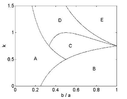
Figure 7: The $(b/a)$ vs. $k$ parameter space for $k=k^{\prime}\neq 1$ at $a=4.0$. Region A: $z^{*}=1/(1+kb)$ stable, B: $z^{*}=1-k$ stable, C: superstable periodic cycles, D: chaos, E: $z^{*}=0$ stable.

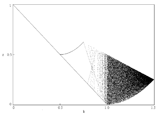
Figure 8: Bifurcation diagram for $k=k^{\prime}\neq 1$ at $a=4.0,b=2.0$.

The bifurcation diagram for $a=4,b=2$ (Fig. 8) shows how the dynamics changes with $k$. For $0\leq k<0.5$, $Z^{*}_{2}=1-k$, is the stable fixed point. At $k=0.5$, $Z^{*}_{2}$ becomes unstable, giving rise to a superstable period-2 cycle. A periodic regime is now observed, which was absent in the previous case. The periodic orbits initially follow a period-doubling sequence until a period-32 ($=2\times 2^{4}$) orbit gives rise to a period-48 ($=3\times 2^{4}$) one. This occurs as a result of border-collision bifurcations by which “period-2 to period-3” bifurcations have been seen to occur [12]. In the above instance, each of the sixteen period-2 orbits give rise to a period-3 orbit. The structure of the superstable periodic orbits is quite complex. The length of the cycles is plotted against $k$ in Fig. 9.

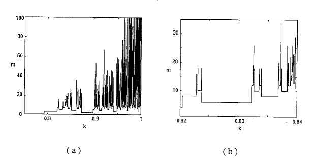
Figure 9: Length of superstable periodic cycles, $m$, of the excitatory-inhibitory neural pair ($a=4$, $b=2$) for (a) 0.75 $\leq$ k $\leq$ 1, and (b) 0.82 $\leq$ k $\leq$ 0.84. Note the self-similar structure of the intervals.

The remarkable self-similar structure of the intervals is to be noted. Numerical studies indicate that cycles of all periods exist having the following ordering: between any superstable period-$m$ and period-$(m+1)$ cycle, there exists an interval of $k$ for which a period-$(m+2)$ orbit is superstable. At $k=1.0$ all periodic orbits become unstable, leading to onset of chaos. The chaotic behavior persists till $k=1.5$, when $Z^{*}_{1}=0$ becomes stable.

Let us now study the effect of introducing a threshold. A positive threshold, $t_{0}>0$, applied to both $F_{a}$ and $F_{b}$, has the effect of shifting the map to the right by $t_{0}$. This allows the segmentation of activation state $(X,Y)$-space, according to dynamical behavior. For initial conditions lying in the region bounded by the two straight lines, $Y=(X-t_{0})/k$ and $Y=(X-t_{0})/(k-1/ak)$, the trajectories are chaotic, provided the maximum point of the map, $F(Z)=1-(kb/a)$, does not iterate into the region $Z>t_{0}+(1/b)$. For the region, $Y>(X-t_{0})/k$, any iterate will map to the fixed point, $Z^{*}=0$. Initial conditions from $Y<(X-t_{0})/(k-1/ak)$ will map to the chaotic region, if the maximum point of the map does not iterate into $Z>t_{0}+(1/b)$. Otherwise, a fractal set of initial conditions will give rise to bounded chaotic motion, the remaining region falling in the “escape set”, eventually leading to periodic orbits.

A negative threshold shifts the map to the left. This has the consequence of destabilizing the fixed point $Z^{*}=0$. If the other fixed point is also unstable then this will imply that all possible $(X,Y)$ values will give rise to periodic or chaotic trajectories. This indicates the possible existence of a global chaotic attractor.

3.3 $k\neq k^{\prime}$

This corresponds to the condition when all the connection weights are different. The dynamics is irreducible to 1-dimension. We need to consider only the positive $(Z,Z^{\prime})$ region, as otherwise, $(0,0)$ is the stable fixed point. In the non-zero region, different dynamical behavior may occur depending on the region where the fixed point occurs and on its stability. One of the fixed points is $(Z,Z^{\prime})=(0,0)$, whose stability is determined by obtaining the eigenvalues of the corresponding Jacobian,

$${\bf J}=\begin{array}[]{|cc|}a&-kb\\ a&-k^{\prime}b\end{array}~{}~{}~{}~{}.$$

Evaluating the above matrix, gives the following condition

$$-2<(a-k^{\prime}b)\pm[(a-k^{\prime}b)^{2}-4ab(k-k^{\prime})]^{1/2}<2,$$ (15)

for stability of the fixed point.

The other fixed point may occur in any one of the four following regions of the $(Z,Z^{\prime})$-space:

Region I: $0<Z<1/a$, $0<Z^{\prime}<1/b$.
$(Z,Z^{\prime})=(0,0)$ is the only fixed point.

Region II: $0<Z<1/a$, $Z^{\prime}>1/b$.
The fixed point is $(Z,Z^{\prime})=(k/(a-1),(a(k-k^{\prime})+k^{\prime})/(a-1))$, which is stable if $-1<a<1$.

Region III: $Z>1/a$, $0<Z^{\prime}<1/b$.
The fixed point is $(Z,Z^{\prime})=((1+b(k^{\prime}-k))/(1+bk^{\prime}),1/(1+bk^{\prime}))$, which is stable if $-1<k^{\prime}b<1$.

Region IV: $Z>1/a$, $Z^{\prime}>1/b$.
The fixed point is $(Z,Z^{\prime})=(1-k,1-k^{\prime})$. This is a superstable root, as the local slope is zero under all conditions.

The abundance of tunable parameters in this case makes detailed simulation study extremely difficult. However, some preliminary studies in the $(k,k^{\prime})$ parameter space (keeping the other parameters fixed) gives indication of dynamics similar to that seen in cases $(i)$ and $(ii)$. The $(k,k^{\prime})$ parameter space is shown in Fig. 10 for $a=4$, $b=2$.

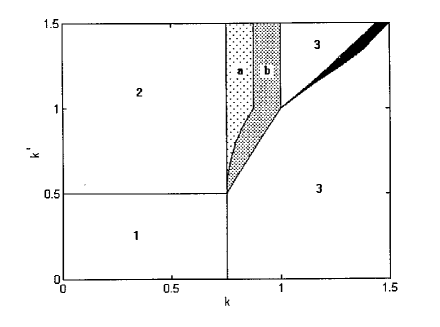
Figure 10: The $(k,k^{\prime})$ parameter space for $a=4.0$ and $b=2.0$. Region 1: $x^{*}$=1, $y^{*}$=1 stable, 2: $x^{*}$=1, $y$ has period-2 cycles, 3: $x^{*}$=0, $y^{*}$=0 stable, $a$: Both $x$ and $y$ have period-2 cycles, $b$: $x$ and $y$ show period-$m$ cycles ($m>2$). Fully chaotic behavior occurs in the dark wedge-shaped region in 3. In addition, fractal intervals showing chaos occur in region $b$.

A variety of dynamical behaviors is observed - from fixed points to periodic cycles to chaos, as indicated by the different regions. In addition, there are regions exhibiting periodic behavior which have fractal intervals of chaotic activity embedded within them.

4 Extension to Large Networks

In the previous section, the behavior of a pair of excitatory-inhibitory neurons (number of neurons, $N=2$) was shown to have sufficient complexity. The dynamics of a N-neuron network ($N>>2$) described by

$${\bf X_{n+1}}=F(\sum{\bf W}.{\bf X_{n})},$$

where ${\bf X_{n}}$ is the set of $N$ activation state values (both excitatory and inhibitory neurons), and ${\bf W}$ is the matrix of connection weights between different neurons. The full range of behavior shown by such a system will be impossible to study in detail, as the number of available tunable parameters are too large to handle. However, under certain restrictions, the dynamics of such large networks can be inferred.

Let $W_{ij}$ denote the connection weight from $j$th to the $i$th neuron. Then, under the condition

$$W_{i~{}j+1}/W_{i~{}1}=k_{j},~{}~{}~{}~{}(k_{j}={\rm constant~{}~{}for~{}~{}a~{}~{}given}~{}~{}j=1,\ldots,N),$$ (16)

the N-neuron network dynamics is reducible to that of a 1-dimensional map with $(N+1)$ linear segments (for $t=0$). The occurrence of “folds” in a map have already been shown to be responsible for creation and persistence of localized coherent structures within a chaotic flow [16]. As in this case, the resultant map will have a number of such folds, the system might show coexistence of multiple chaotic attractors (isolated from each other). A simple example to illustrate this point is a fully connected network of four neurons: two excitatory ($x_{1}$,$x_{2}$) and two inhibitory ($y_{1}$,$y_{2}$). Let $a_{i}$ and $b_{i}$ represent the slope of the transfer functions for the $i$th excitatory and inhibitory neurons, respectively. The 4-dimensional dynamics is reducible to the 1-dimensional dynamics of $z=x_{1}-k_{1}y_{1}+k_{2}x_{2}-k_{3}y_{2}$. Simulations were carried out for the set of parameter values: $(a_{1}=4.6,a_{2}=4.0,b_{1}=3.6,b_{2}=1.6)$ and $(k_{1}=0.7,k_{2}=1.0,k_{3}=1.1)$. Furthermore, $x_{2}$,$y_{2}$ have a threshold equal to $1/b_{1}$. Fig. 11(a) shows the return map and time evolution of $z$ in the absence of any bias. There is only a single global chaotic attractor in this case. When a small negative bias is applied to the whole network, the previous attractor splits into two coexisting isolated attractors having localized chaotic activity. Which attractor the system will be in, depends upon the initial value it starts from.

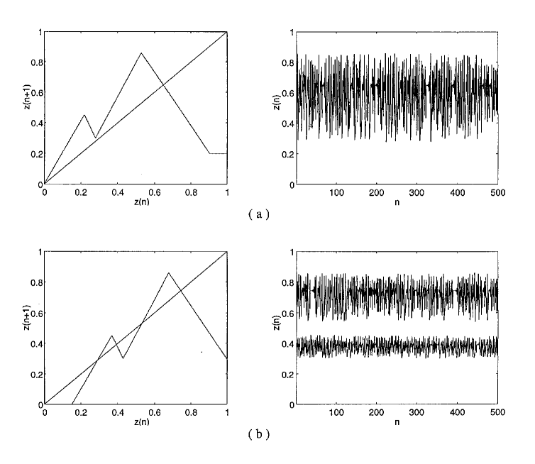
Figure 11: The return map and time evolution of the reduced variable, $z$, for a 4-neuron network (for details see text), with (a) bias = 0 and (b) bias = – 0.15. In the former there is a single global chaotic attractor. For non-zero bias, there are two co-existing chaotic attractors. Time evolution of $z$ starting from two initial conditions belonging to different attractors are superposed.

Fig. 11(b) shows the return map for a bias value of -0.15 and the superposed time evolutions of $z$ starting from initial conditions belonging to two different attractors. So, an increase in bias, can cause transition from global chaos to localized chaotic regions.

This property can be used to simulate a proposed mechanism of olfactory information processing [1]. It has been suggested that the olfactory system maintains a global attractor with multiple “wings”, each corresponding to a specific class of odorant. During each inhalation, the system moves from the central chaotic repeller to one of the wings, if the input contains a known stimulus. The continual shift from one wing to another via the central repelling zone has been termed as chaotic “itinerancy”. This forms the basis of several chaotic associative memory models.

The above picture can be observed in the present model by noting that, if the external input has the effect of momentarily increasing the bias from a negative value to zero, then the isolated chaotic regions merge together into a single global attractor. In this condition, the entire region is accessible to any input state. However, as the bias goes back to a small negative value, the different isolated chaotic attractors re-emerge, and the system dynamics is constrained into one of these. Sustained external stimuli will cause the gain parameters to decrease (adaptation), thereby decreasing the local slope of the map. If the stimulus is maintained, the unstable fixed point in the isolated region will become stable leading to a fixed-point or periodic behavior. The above scenario, in fact, is the basis of using the proposed model as an associative memory network.

5 Information Processing with Chaos

Chaotic dynamics enables the microscopic sensory input received by the brain to control the macroscopic activity that constitutes its output. This occurs as a result of the selective sensitivity of chaotic systems to small fluctuations in the environment and their capacity for rapid state transitions. On the other hand, chaotic attractors are globally extremely robust. These properties indicate that the utilization of chaos by biological systems for information processing can indeed be advantageous. It has been suggested, based on investigations into cellular automata, that complex computational capabilities emerge at the “edge of chaos” [17].

Based on this notion, efforts are on to use chaos in neural network models to achieve human-like information processing capabilities. Chaotic neural networks have been already been applied in designing associative memory networks [6] and solving combinatorial optimization problems, using chaos to carry out an effective stochastic search [3]. The superposition of chaotic maps for information processing has also been suggested before [18].

The model presented in this paper can be used for a variety of purposes, classified as follows:

Associative memory: A set of patterns (i.e., specific network state configurations) are stored in the network as attractors of the system dynamics, such that, whenever a distorted version of one of the patterns is presented to the network as input, the original is retrieved upon iteration. The distortion has to be small enough so that the input pattern is not outside the basin of attraction of the desired attractor. In networks using convergent dynamics, the stored patterns necessarily have to be time-invariant or at most, periodic.

Chaos provides rapid and unbiased access to all attractors, any of which may be selected on presentation of a stimulus, depending upon the network state and external environment. It also acts as a “novelty detector”, classifying a stimulus as being previously unknown, by not converging to any of the existing attractors. This suggests the use of chaotic networks for auto association.

In the previous section, the basic mechanism for constructing an associative memory network has been described. In this proposed model, both constant and periodic sequences can be stored. This is made possible by introducing “folds” in the return map of the network, so that a large number of isolated regions are produced. The nature of the dynamics in a region can be controlled by altering the gain parameters of individual neurons. Accessibility to a given attractor depends upon the initial condition of the network and the input stimulus. So, regions with fixed-point or periodic attractors may be embedded within regions having chaotic behavior. In addition, chaotic trajectories confined within a specific region can also be generated when presented with a short-duration input stimulus belonging to that region. “Novelty detection” is implemented in the above model by making the basins of attractors (corresponding to the stored patterns) of some pre-specified size. Input belonging outside the region, therefore, cannot enter the basin and will not be able to converge to the stored pattern.

Pattern classification: In this information processing task, different input sets need to be classified into a fixed number of categories. Decision boundaries, i.e., boundaries between the different classes are constructed by a “training session” where the network is presented with a series of inputs and the corresponding class to which they belong. In the proposed model, classification can be on the basis of dynamical behavior. For example, input sets belonging to different input classes may give rise to different periodic sequences. Otherwise, the distinction can be made between categories of inputs which give rise to chaotic and non-chaotic trajectories. For a pair of neurons ($N=2$), under the condition $k=k^{\prime}$, linear separation of the $(X,Y)$-space can be done (as shown above). By varying the parameters $k$ and $b$, the orientation and size of the class regions can be controlled. If $k\neq k^{\prime}$ and $N>2$, nonlinear decision boundaries between different classes can be generated. By using suitably adjusted weights, any arbitrary classification can be achieved.

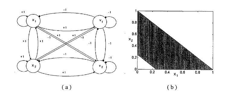
Figure 12: (a) A fully connected 4-neuron network with 2 excitatory ($x_{1,2}$) and 2 inhibitory ($y_{1,2}$) neurons. The arrows and circles represent excitatory and inhibitory synapses, respectively. (b) The $(x_{1},x_{2})$ phase space shows the basin of the chaotic attractor (shaded region) for threshold, $t$=0.25. The unshaded region corresponds to fixed point behavior of the network.

An example of nonlinear decision boundary generation is shown in Fig. 12. The network used for this purpose consists of 4 neurons - 2 excitatory ($x_{1},x_{2}$) and 2 inhibitory ($y_{1},y_{2}$) (fig. 12(a)). The gain parameters are $a_{x_{1},x_{2}}=2$ and $b_{y_{1},y_{2}}=1$. All the neurons have a threshold, $t$. The network is fully connected with all weightages equal to unity. The input stimulus is taken to be the initial value of the excitatory neurons and the inhibitory neuronal states are initially taken to be zero.

As shown in fig. 12(b), for $t$ = 0.25, the $(x_{1},x_{2})$ phase space is segmented into basins leading to either fixed point or chaotic attractors. By increasing $t$, the width of the chaotic band can be reduced. Changing the initial value of the inhibitory neurons will cause translation of the band and manipulating the connection weights gives a rotation to the band. Thus, any general transformation can be applied to the segment. More complex network connections might permit segmenting isolated box-like regions in the phase space. This possibility is currently under investigation.

System Dynamics Approximation: A system may be described by a nonlinear input-output relation,

$$Y={\bf G}(X),$$

where the mapping function, ${\bf G}$, is unknown. By having access to a limited set of input-output pairs, the function has to be approximated - in effect, building a system simulator. In the present model, a sufficient number of coupled neurons can be used to construct any arbitrary piecewise linear input-output relation. By use of a suitable learning rule, the available data set can be used to determine the gain parameters, thresholds and connection weights of the network. A close approximation of the system dynamics will enable prediction and control of its behavior. The approximation’s accuracy is not restricted to systems with piecewise linear functions - but can also give good qualitative reconstruction of smooth nonlinear systems.

Periodic sequence generation: Capability for periodic sequence generation can be exploited for modeling central pattern generators. These are a class of biological neural ensembles which control well-defined rhythmic muscle movements such as swimming, running, walking, breathing, etc. Usually they are found in the spinal cord, producing periodic sequences without feedback from the motor system or higher-level control. The ability to generate multiple sequences from the same neural assembly is another interesting feature. Postulating the existence of single pacemaker neurons acting as the ‘system clock’ to initiate periodic activity cannot explain all the observed phenomena. The existing network models for simulating this behavior mostly suffer from the drawback that they cannot generate multiple non-overlapping sequences. This shortcoming is overcome in the model presented here. For $N=2$ and $k=k^{\prime}\neq 1$, a rich variety of periodic sequences can be chosen from the same network, simply by altering the gain parameters by a very small amount. As mentioned above, numerical investigations indicate that cycles of any period can be generated by suitably altering the value of $k$.

6 Discussion and Future Work

The network has been studied in detail only for $N=2$. Nonetheless it shows capability for supporting extremely complex behavior. Under certain restrictions, the dynamics for $N>>2$ networks can also be understood. Relaxation of these restrictions will provide a challenging task for the future.

One important point not touched here is the issue of learning. The connection weights {$W_{ij}$} have been assumed constant, as they change at a much slower time scale compared to that of the activation state values. However, modification of the weights due to learning will also cause changes in the dynamics. Such bifurcation behavior, induced by weight changes, will have to be taken into account when devising learning rules for specific purposes. The interaction of chaotic activation dynamics at a fast time scale and learning dynamics on a slower time scale might yield richer behavior than that seen in the present model. An interesting study for the future will be to introduce time-varying Hebbian synaptic weights, evolving according to

$$W_{ij}(n+1)=W_{ij}(n)+\epsilon X_{i}(n)X_{j}(n),$$

where $X(n)$ and $W(n)$ denote the neuron state and connection weight at the $n$th instant, and $\epsilon$ is related to the time-scale of the synaptic dynamics. The combined effect of such synaptic dynamics with the chaotic network dynamics (for small $N$) described above might lead to significant departure from the overall features described here.

Real biological systems reside in an extremely noisy environment. This is incorporated into neural models by using stochastic updating rule and/or explicit introduction of a term representing external noise. We plan to introduce similar features in the proposed model. In dissipative chaotic systems, the effect of external noise seems to be limited to destroying the fine structure of the bifurcation sequence [19]. The interaction of deterministic chaos and stochastic noise in the network will be interesting to study.

Another possible modification to the present model will be to incorporate time-varying operating conditions. In [8] time-dependence of a suitable system parameter was shown to give rise to interesting dynamical behaviors, e.g., transition between periodic oscillations and chaos. This suggests that varying the environment can facilitate memory retrieval if dynamic states are used for storing information in a neural network. In the proposed network, periodic variations can be incorporated into the available system parameters: gain, threshold and connection weights. In nonlinear systems, time-varying dynamics often leads to the phenomenon of “stochastic resonance” where a subthreshold signal is amplified by the background noise. It has been observed that replacing noise by chaos also gives rise to this resonance behavior in a bimodal piecewise linear map [20]. It will be of interest to see whether such phenomena can occur in the present model, on the introduction of temporal variation in the parameters. The occurrence of “resonance” might enhance the capability of the network to detect subthreshold signals, through signal amplification by deterministic ‘noise’.

References

- [1] W. J. Freeman, “Tutorial on neurobiology: from single neurons to brain chaos,” Int. J. Bif. and Chaos, 2, 1992, pp. 451–482.
- [2] X. Wang, “Period-doublings to chaos in a simple neural network: an analytical proof,” Complex Systems, 5, 1991, 425–441.
- [3] M. Inoue and S. Fukushima, “A neural network of chaotic oscillators,” Prog. Theor. Phys., 87, 1992, 771–774.
- [4] I. Tsuda, “Dynamic link of memory: chaotic memory map in nonequilibrium neural networks,” Neural Networks, 5, 1992, 313–326.
- [5] Y. V. Andreyev, Y. L. Belsky, A. S. Dmitriev and D. A. Kuminov, “Information processing using dynamical chaos: neural networks implementation,” IEEE Trans. on Neural Networks, 7, 1996, 290–299.
- [6] S. Ishii, K. Fukumizu and S. Watanbe, “A network of chaotic elements for information processing,” Neural Networks, 9, 1996, 25–40.
- [7] S. Sinha, “Controlled transition from chaos to periodic oscillations in a neural network model,” Physica A, 224, 1996, 433–446.
- [8] L. Wang, “Oscillatory and chaotic dynamics in neural networks under varying operating conditions,” IEEE Trans. on Neural Networks, 7, 1996, 1382–1388.
- [9] H. E. Nusse and J. A. Yorke, “Border-collision bifurcations for piecewise smooth one-dimensional maps,” Int. J. Bif. and Chaos, 5, 1995, 189–207.
- [10] H. R. Wilson and J. D. Cowan, “Excitatory and inhibitory interactions in localized populations of model neurons,” Biophys. J., 12, 1972, 1–24.
- [11] N. J. Schulmann, “Chaos in piecewise linear systems,” Phys. Rev. A, 28, 1983, 477–479.
- [12] H. E. Nusse and J. A. Yorke, “Border-collision bifurcations including “period-two to period-three” for piecewise smooth systems,” Physica D, 57, 1992, 39–57.
- [13] J. L. McCauley, Chaos, dynamics and fractals. Cambridge: Cambridge Univ. Press, 1993.
- [14] C. Grebogi, E. Ott and J. A. Yorke, “Crises, sudden changes in chaotic attractors and chaotic transients,” Physica D, 7, 1983, 181–200.
- [15] T. Yoshida, H. Mori and H. Shigematsu, “Analytic study of the tent map: band structures, power spectra and critical behaviors,” J. Stat. Phys., 31, 1983, 279–308.
- [16] T. Shinbrot and J. M. Ottino, “Using horseshoes to create coherent structures,” Phys. Rev. Lett., 71, 1993, 843–846.
- [17] C. G. Langton, “Computation at the edge of chaos: phase transitions and emergent computation,” Physica D, 42, 1990, 12–37.
- [18] Y. V. Andreyev, A. S. Dmitriev and S. O. Starkov, “Information processing in one-dimensional systems with chaos,” IEEE Trans. on Circuits and Systems - I, 44, 1997, 21–28.
- [19] J. Crutchfield, M. Nauenberg and J. Rudnick, “Scaling for external noise at the onset of chaos,” Phys. Rev. Lett., 46, 1981, 933–935.
- [20] S. Sinha and B. K. Chakrabarti, “Deterministic SR in a piecewise linear chaotic map.” Phys. Rev. E, 58, 1998, 8009–8012.