[

Statistical Theory of Energy Transfer to Small and Chaotic Quantum Systems Induced by a Slowly-Varying External Field

Abstract

We study nonequilibrium properties of small and chaotic quantum systems, i.e., non-integrable systems whose size is small in the sense that the separations of energy levels are non-negligible as compared with other relevant energy scales. The energy change $\Delta E$ induced by a slowly-varying external field $\lambda(t)$ is evaluated when the range of the variation $\Delta\lambda$ is large so that the linear response theory breaks down. A new statistical theory is presented, by which we can predict $\langle\Delta E\rangle$, the average of $\Delta E$ over a finite energy resolution $\delta E$, as a function of $\lambda(t)$ if we are given the density of states smeared over $\delta E$, the average distance of the anticrossings, and a constant $K\lesssim 1$.

]

Recently, active research has been devoted to small and chaotic quantum (SCQ) systems, i.e., non-integrable systems whose size is small in the sense that the separations of energy levels are non-negligible as compared with other relevant energy scales [2]. Such systems are frequently encountered in many fields of physics [2], such as excited states of molecules [3] and those of quantum dots [4]. SCQ systems have the universal properties that level spacings obey a universal distribution, and that the energy levels exhibit anticrossings as a function of an external parameter $\lambda$ [2]. Note that these are static properties. In contrast, only limited knowledge has been obtained for dynamical or nonequilibrium properties of SCQ systems [5]. A major difficulty is that solving the time-dependent Schrödinger equation (TDSE) becomes impossible when $f\gtrsim 4$, where $f$ is the degrees of freedom of the system, for the most common case where the “coordinate” of each degree of freedom takes continuous values. This is because the computational time generally grows exponentially with $f$. If $f$ were huge enough, on the other hand, the nonequilibrium thermodynamics would be applicable, by which one could predict nonequilibrium properties much more easily than by solving the TDSE. For SCQ systems, however, the nonequilibrium thermodynamics is not applicable because its basic assumptions, such as the local equilibrium, are not satisfied. The purpose of the present Letter is to propose a new theory, called the random-probability netweork (RPN) method, by which nonequilibrium properties of SCQ systems can be predicted easily, without solving the TDSE [6].

We consider an SCQ system subject to an external field $\lambda(t)$, which represents any external disturbance, such as a magnetic or electric field, and the position coordinate of a moving “wall” (a portion of another system which couples to the SCQ system). The energy change $\Delta E$ induced by the variation of $\lambda(t)$ [7] is evaluated under the conditions that (i) the range of the variation $\Delta\lambda$ is large so that $\Delta\lambda$ cannot be treated as a small perturbation and the linear response theory breaks down, and that (ii) the typical time scale $T$ of the variation of $\lambda$ is long (so that $r$ of Eq. (5) $\ll 1$). Without solving the TDSE, we can easily predict $\langle\Delta E\rangle$, the average of $\Delta E$ over a finite energy resolution $\delta E$, by the RPN method if we are given a constant $K$ ($\lesssim 1$) and two “fundamental functions” which contain only small information of the system.

To be concrete, we explain the RPN method using a simple model. However, since the basic idea is based on the universal properties mentioned above, we expect that the RPN method is generally applicable to SCQ systems. Consider the time evolution of coupled rotators (angular momenta $\hat{\bf L}$ and $\hat{\bf M}$), whose Hamiltonian is [8]

$$\hat{\cal H}(t)=\lambda(t)\left(\hat{L}_{z}+\hat{M}_{z}\right)+\hat{L}_{x}\hat{M}_{x}\equiv\hat{\cal H}_{1}(t)+\hat{\cal H}_{2},$$ (1)

in an appropriate unit system, in which the energy, $\lambda$ and $\hbar$ are dimensionless [8]. The external field $\lambda(t)$ is taken as $\lambda(t)=1-\Delta\lambda[1-(t/T)^{2}]^{4}$ for $-T\leq t\leq T$ and $\lambda(t)=1$ for $|t|>T$ [9]. Since we are interested in the case where $\Delta\lambda$ is large, we here take $\Delta\lambda=0.5$. For this $\lambda(t)$, $\hat{\cal H}$ takes the same form at both ends, $t=\pm T$, and $\Delta E$ can be finite only when transitions occur between different levels. However, it should be stressed that the RPN method is also applicable to the case of $\hat{\cal H}(T)\neq\hat{\cal H}(-T)$, for which $\langle\Delta E\rangle$ consists of both the shifts of energy levels and the transitions between them.

As in the case of the statistical mechanics, we must first classify quantum states according to constants of motion, to obtain a set of subspaces, each of which has no constant of motion. It is in each subspace that the system has chaotic natures and the RPN method is applicable. We here consider the subspace of $J_{z}/\hbar=even$, $l=m=15$, $\Sigma=+$. Here, $J_{z}\equiv L_{z}+M_{z}$, $\hbar^{2}l(l+1)$ and $\hbar^{2}m(m+1)$ are the quantized values of $\hat{L}^{2}$ and $\hat{M}^{2}$, and $\Sigma$ denotes the parity under the exchange of $L_{z}$ and $M_{z}$. We take $\hbar=0.322748612$, so that the corresponding classical system is chaotic [8]. The eigenvalues $E_{n}(\lambda)$ exhibit anticrossings as functions of $\lambda$ as shown in Fig. 1. In the inset of Fig. 2, we plot the density of states $\rho_{\delta E}(E;\lambda)$ which is smeared over a finite energy range $\delta E$. Here and after, we consider the $E<0$ part only, because the system is symmetric about $E=0$. On an average, $\rho_{\delta E}(E;\lambda)$ is an increasing function of $E$ for $E<0$ (whereas it is decreasing for $E>0$), and the average energy spacing ($=1/\rho_{\delta E}$) decreases with $E$. We have confirmed that the normalized spacing, $s_{n}(\lambda)\equiv\rho_{\delta E}(E;\lambda)(E_{n+1}(\lambda)-E_{n}(\lambda))$, obeys the Wigner distribution, $P(s)\simeq(\pi s/2)\exp(-\pi s^{2}/4)$ [2].

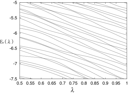
FIG. 1.: The energy levels as a function of $\lambda$.

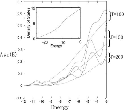
FIG. 2.: The integrated energy change $A_{\delta E}(E)$ for $T=$ 100, 150, 200, obtained by solving the TDSE (solid lines) and by the RPN method (dashed lines). Inset: The smeared density of states $\rho_{\delta E}(E;\lambda)$ for $\lambda=1.0$, $\delta E=1.0$.

Before presenting the RPN method, we first explore dynamical properties of the system by numerically solving the TDSE, $\imath\hbar\frac{\partial}{\partial t}|\psi(t)\rangle=\hat{\cal H}(t)|\psi(t)\rangle.$ Here, we use the split operator method [10] to obtain the time evolution operator $\hat{U}(t_{2},t_{1})$ defined by $|\psi(t_{2})\rangle=\hat{U}(t_{2},t_{1})|\psi(t_{1})\rangle.$ Noting that $\hat{\cal H}(t)$ is constant for $|t|\geq T$, we take one of its eigenstates $|\psi_{n}\rangle$, where $\hat{\cal H}(|t|\geq T)|\psi_{n}\rangle=E_{n}|\psi_{n}\rangle$, as the initial state. The state at $t\geq-T$ is denoted by $|\psi_{[n]}(t)\rangle\equiv\hat{U}(t,-T)|\psi_{n}\rangle.$ We are interested in the energy change $\Delta E_{n}$ between the initial ($t=-T$) and the final ($t=T$) states [7]; $\Delta E_{n}\equiv\langle\psi_{[n]}(T)|\hat{\cal H}(T)|\psi_{[n]}(T)\rangle-E_{n}.$ This is plotted against $E_{n}$ for $T=100$ in Fig. 3. It is seen that $\Delta E_{n}$ scatters rather randomly as a function of $E_{n}$. It is therefore impossible to predict $\Delta E_{n}$ of individual levels, without solving the TDSE.

FIG. 3.: The energy change for $T=100$, as a function of the initial energy $E_{n}$.

To see what predictions are possible and meaningful, let us consider typical experiments on SCQ systems. Suppose that one tries to prepare the initial state in $|\psi_{n}\rangle$. However, except for the ground state, it is difficult to prepare the initial state of SCQ systems accurately. Hence, one can actually prepare the initial state in a finite energy range $E_{n}-\delta E/2\leq E\leq E_{n}+\delta E/2$, where $\delta E$ denotes the energy resolution of the apparatus. Therefore, the initial state should be an incoherent mixture or a coherent superposition of $|\psi_{m}\rangle$’s of $|E_{m}-E_{n}|\lesssim\delta E/2$. Let $\Delta E_{\delta E}^{(j)}(E)$ be the measured value of the energy change in the $j$th one of such experiments, where $E=E_{n}$. This quantity fluctuates from experiment to experiment for two reasons: One is the random fluctuation of $\Delta E_{n}$ as a function of $E_{n}$ mentioned above; this fluctuation appears in $\Delta E_{\delta E}^{(j)}(E)$ because the intial state is prepared randomly in the energy range $|E_{m}-E|\lesssim\delta E/2$. The other reason is the quantum-mechanical fluctuation; even if $\delta E\to 0$, only the average of $\Delta E_{\delta E}^{(j)}(E)$ over many experiments would agree with $\Delta E_{n}$. Namely, even for the same initial state $|\psi_{n}\rangle$, the measured value of each experiment scatters about $\Delta E_{n}$, with the standard deviation, $D_{n}\equiv[\langle\psi_{[n]}(T)|(\hat{\cal H}(T)-E_{n})^{2}|\psi_{[n]}(T)\rangle-(\Delta E_{n})^{2}]^{1/2}.$ By numerically computing $D_{n}$, we find that $D_{n}\sim\Delta E_{n}$. Because of these large fluctuations, a single experiment is insufficient for comparison of the experimental result with a theoretical one, for an SCQ system. We must therefore perform many experiments, and we are most interested in the average $\Delta E_{\delta E}(E)$ of their results. We will argue later, and have confirmed numerically, that the quantum coherence of the initial state is irrelevant to this quantity, under our assumption that $\Delta\lambda$ is large so that the system experiences many anticrossings during the variation of $\lambda$. Therefore, $\Delta E_{\delta E}(E)$ equals the average of $\Delta E_{m}$’s over $m$’s which satisfies $|E_{m}-E|\lesssim\delta E/2$;

$$\Delta E_{\delta E}(E)\simeq\frac{\displaystyle{\int_{E-\delta E/2}^{E+\delta E/2}d\epsilon\sum_{m}\Delta E_{m}\phi_{\delta E}(\epsilon-E_{m})}}{\displaystyle{\int_{E-\delta E/2}^{E+\delta E/2}d\epsilon\sum_{m}\phi_{\delta E}(\epsilon-E_{m})}},$$ (2)

where $\phi_{\delta E}(\epsilon)$ is the normalized gaussian function with width $\delta E$. To find statistical tendencies of $\Delta E_{\delta E}(E)$, we investigate the integrated energy change defined by

$$A_{\delta E}(E)\equiv\int_{-\infty}^{E}d\epsilon\cdot\sum_{n}\Delta E_{n}\phi_{\delta E}(\epsilon-E_{n}).$$ (3)

We can obtain $\Delta E_{\delta E}(E)$ from $A_{\delta E}(E)$ as

$$\frac{A_{\delta E}(E+\delta E/2)-A_{\delta E}(E-\delta E/2)}{\rho_{\delta E}(E)\delta E}=\Delta E_{\delta E}(E).$$ (4)

We plot $A_{\delta E}(E)$ for $\delta E=1.0$, as a function of $E$, by the solid lines in Fig. 2. We find that $A_{\delta E}(E)$ is a smooth and, on an average, increasing function of $E$. It strongly suggests that the prediction about $A_{\delta E}(E)$ may be possible by a simple theory, without solving the TDSE.

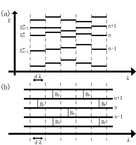
FIG. 4.: A pair of the RPN diagrams (a) and (b).

As such a theory we now present the RPN method, by which we can calculate $A_{\delta E}(E)$ (hence $\langle\Delta E\rangle$) as a function of $\lambda(t)$, if we are given a constant $K$ and two “fundamental functions,” which are $\rho_{\delta E}(E;\lambda)$ and the average distance $\lambda_{s}(E;\lambda)$ (along the $\lambda$ axis of Fig. 1) of the anticrossings [11]. Note that these functions contain only small information on the system because they represent the distribution of energy levels only, and further loss of information occurs by averaging it over a finite energy $\delta E$. The RPN method enables us to predict $A_{\delta E}(E)$ from such small and reduced information.

The RPN method is applicable under the conditions that (i) $\Delta\lambda$ is large so that each level encounters many anticrossings from $t=-T$ to $T$, and that (ii) $T$ is long so that most transitions between different levels occur only at anticrossings, and the transition at each anticrossing occurs only between adjacent levels. (This is satisfied if $r$ of Eq. (5) $\ll 1$.) Both conditions are satisfied for $\Delta\lambda=0.5$ and $T\gtrsim 100$ for the present model. Under these conditions, anticrsossings may be regarded as “bridges,” only through which transitions occur, and the RPN method is formulated as follows.

Step 1: Associate the level diagram of the original system, Fig. 1, with many pairs of hypothetical diagrams, which we call the RPN diagrams. Each pair consists of two diagrams (a) and (b), as shown in Fig. 4. Diagram (a) is a set of hypothetical energy levels $E_{1}^{*},E_{2}^{*},\cdots,E_{N}^{*}$, where the number $N$ of the levels are taken equal to or larger than the number of relevant energy levels. In each small interval $[\lambda,\lambda+d\lambda)$, the hypothetical levels are generated randomly according to $\rho_{\delta E}(E;\lambda)$ of the original system and the Wigner distribution of the spacings. Here, the small interval $d\lambda$ is taken in such a way that $d\lambda/\lambda_{s}(E_{n}^{*}(\lambda);\lambda)\ll 1.$ Diagram (b) is a set of straight lines (labeled by $n=1,2,\cdots$) with “bridges” (labeled by $B_{1},B_{2},\cdots$). The bridges are randomly generated in such a way that the probability of finding one bridge in each small interval $[\lambda,\lambda+d\lambda)$ on line $n$ is given by $d\lambda/\lambda_{s}(E_{n}^{*}(\lambda);\lambda)$, where $E_{n}^{*}(\lambda)$ is given by diagram (a). We also impose the condition that any two bridges are not on a single line in the same interval. This constriction is consistent with the assumption $d\lambda/\lambda_{s}\ll 1,$ which states that the probability of finding such two bridges in the original system is negligible.

Step 2: Attach an $N\times N$ matrix w to each bridge, where ${\bf w}(B)$ at a bridge $B$ between lines $n$ and $n+1$ is given by $w_{n,n+1}=w_{n+1,n}=r,$ $w_{n,n}=w_{n+1,n+1}=1-r,$ and $w_{i,j}=w_{j,i}=\delta_{i,j}$ for $i\neq n,n+1$. Here, $r\equiv r((E_{n}^{*}+E_{n+1}^{*})/2;\lambda)$ represents the transition probability at the bridge, where

$$r(E;\lambda)\equiv\exp\left[-{2\pi K^{2}}{\lambda_{s}(E;\lambda)}/{\hbar|\dot{\lambda}}|{\rho_{\delta E}(E;\lambda)}\right].$$ (5)

Here, $K$ is a constant ($\lesssim 1$), which is considered as a fundamental parameter of the RPN method. This form of $r(E;\lambda)$ is deduced from the Landau-Zener formula for two levels; $r=\exp(-{2\pi V^{2}}/{\hbar|\dot{\lambda}|}{|F_{1}-F_{2}|})$. Here, by replacing the difference $|F_{1}-F_{2}|$ between the slopes of the levels with $K_{2}/\rho_{\delta E}(E;\lambda)\lambda_{s}$, and the energy gap $V$ at the anticrossing with $K_{3}/\rho_{\delta E}(E;\lambda)$, where $K_{2}\simeq 1$ and $K_{3}\lesssim 1$, we arrive at Eq. (5) with $K=K_{3}/\sqrt{K_{2}}\lesssim 1$.

Step 3: Construct an $N\times N$ matrix W as follows. Draw the vertical line at $\lambda=\lambda(-T)$ in diagram (b). Associate the vertical line with the matrix W, and take it as the unit matrix. Move the vertical line as a function of $t$, according to $\lambda=\lambda(t)$. When the vertical line encounters a bridge $B$, multiply ${\bf W}$ by ${\bf w}(B)$ of the bridge: ${\bf W}\to{\bf w}(B){\bf W}.$ If the line encounters two or more bridges simultaneously, multiply ${\bf W}$ by ${\bf w}$’s of the bridges, where, the order of ${\bf w}$’s are arbitrary because such ${\bf w}$’s of the bridges on the same vertical line commute with each other. In this way, ${\bf W}$ at the final time ($t=T$) becomes the product of ${\bf w}(B)^{\prime}s$ along the “path” of $\lambda(t)$. We interpret its element $W_{mn}$ as the probability of the transition from line $n$ at $t=-T$ to line $m$ at $t=T$, of the random probability network.

Step 4: Evaluate the average change of the hypothetical energy by $\Delta E_{n}^{*}\equiv\sum_{m}(E_{m}^{*}(\lambda(T))-E_{n}^{*}(\lambda(-T))W_{mn},$ which is the counterpart of $\Delta E_{n}$ of the original system. Calculate the integrated energy change of the RPN by

$$A_{\delta E}^{*}(E)\equiv\int_{-\infty}^{E}d\epsilon\cdot\sum_{n}\Delta E_{n}^{*}\phi_{\delta E}(\epsilon-E_{n}^{*}).$$ (6)

Step 5: Repeat steps 1-4 many times, to obtain many $A_{\delta E}^{*}(E)$’s, which correspond to different pairs of the RPN diagrams. Calculate the average of $A_{\delta E}^{*}(E)$’s. This average is the result for $A_{\delta E}(E)$ by the RPN method.

The total computational time is tremendously reduced as compared with solving the TDSE; e.g., from a few days to a few seconds for the model of Eq. (1). The reduction becomes much more drastic as $f$ is increased.

To check the validity of the RPN method, we compare $A_{\delta E}(E)$ of the RPN method with that obtained by solving the TDSE. In the RPN method we use $\rho_{\delta E}(E;\lambda)$ and $\lambda_{s}(E;\lambda)$ that are obtained by solving the time-independent Schrödinger equation. The constant $K$ is determined so as to optimize the agreement between the results of the RPN method and the TDSE. (Hence, $K$ is the only free parameter in the comparison.) This gives $K=0.177$, in consistent with $K\lesssim 1$. The dashed lines in Fig. 2 plot $A_{\delta E}(E)$ obtained by the RPN method for various values of $T$. On an average, they agree with the solid lines obtained by solving the TDSE, although the fine structures, peaks and dips, of the solid lines are absent in the dashed lines. It is expected that such peaks and dips would be shallower for larger systems. Considering also the tremendous reduction of the computaional time, the overall agreement seems satisfactory. The reason why the RPN method gives good results is partly that we have introduced the finite energy resolution $\delta E$, which results in the average over many initial states. This smears out strong dependence on the initial state. Another reason is that we have assumed a large value of $\Delta\lambda$. As a result, the wavefunction experiences many anticrossings under the variation of $\lambda(t)$, and effects of the phase coherence on $\langle\Delta E\rangle$ are almost destroyed on an average. Detailed discussions on this point will be described elsewhere.

As we have done above, we may obtain the fundamental functions by solving the time-independent Schrödinger equation, which is much easier than solving the TDSE. For larger systems, or for systems whose Hamiltonian is unknown, the fundamental functions and $K$ may be obtained from some experiments (e.g., on the specific heat) and/or experiences (in similar systems), as in the case of estimating thermodynamical functions from experiments. To develop a systematic method to perform this program is a subject of future study.

We finally note that $A_{\delta E}(E)$ is, on an average, an increasing function of $E$. This means that if $\lambda(t)$ is varied repeatedly, then, as a result of accumurated transitions, the energy of the system tends toward $E=0$, where $\rho_{\delta E}(E)$ is highest. We thus find that the system tends to “climb” the curve of the smeared density of state. Therefore, an SCQ system tends to absorb the energy if its $\rho_{\delta E}(E)$ is an increasing function of $E$.

REFERENCES

- [1] Contact author: E-mail: shmz@ASone.c.u-tokyo.ac.jp
- [2] See, e.g., papers in Prog. Theoret. Phys. (Kyoto), Suppl. 116 (1994).
- [3] See, e.g., N. Hashimoto and K. Takatsuka, J. Chem. Phys. 103 (1995) 6914.
- [4] See, e.g., O. Agam et al., Phys. Rev. Let. 78, 1956 (1997).
- [5] R.V. Jensen and R. Shanker, Phys. Rev. Let. 54, 1879 (1985); S. Miyashita, J. Phys. Soc. Jpn. 64 (1995) 3207; M. Wilkinson and E. J. Austin, J. Phys. 28, 2277 (1995), and references cited therein.
- [6] The RPN method should not be confused with the theories of P. Pechukas, Phys. Rev. Lett. 51, 943 (1983) and T. Yukawa, ibid 54, 1883(1985). They discussed static properties of SCQ systems by regarding the qauntum levels as trajectories of classical gas particles.
- [7] The energy change equals the energy transfer between the SCQ system and the external system that causes the variation of .
- [8] This model with a time-independent was analyzed, e.g., in M. Feingold, N. Moiseyev and A. Peres, Phys. Rev. A30, 509 (1984). The thermalization was analyzed in F. Borgonovi et al., Phys. Rev. E57, 5291 (1998).
- [9] Some models, such as kicked rotors, have singularies in the dependence of or . However, such singularities should not be present in real physical systems. The RPN method is applicable to the latter case. Although of Eq. (1) has weak singularities at , we have confirmed numerically that their effects are negligible for the values of assumed in the present paper.
- [10] K. Takahashi and K. S. Ikeda, J. Chem. Phys. 99, 8680 (1993).
- [11] The average is taken over and , where is taken large enough ( here) so that is well defined.