Spatiotemporal Chaos, Localized Structures and Synchronization in the Vector Complex Ginzburg-Landau Equation

We study the spatiotemporal dynamics, in one and two spatial dimensions, of two complex fields which are the two components of a vector field satisfying a vector form of the complex Ginzburg-Landau equation. We find synchronization and generalized synchronization of the spatiotemporally chaotic dynamics. The two kinds of synchronization can coexist simultaneously in different regions of the space, and they are mediated by localized structures. A quantitative characterization of the degree of synchronization is given in terms mutual information measures.

To appear in International Journal of Bifurcation and Chaos (1999). A version with higher quality figures could be found at http://www.imedea.uib.es/PhysDept/publicationsDB/date.html

1 Introduction

Starting from the pioneering experimental study by Huygens with two marine pendulum clocks hanging from a common support [Huygens, 1665], synchronization phenomena have been subject of intense study in many physical and biological systems [Winfree, 1980, Strogatz and Steward, 1993]. Since [Pecora and Carroll, 1990] established that chaotic oscillators can also become synchronized, many applications and extensions of the original idea have been identified. Some of them are the possibilities of partial (i.e. phase) synchronization [Rosenblum et al., 1996], generalized synchronization [Rulkov et al., 1995, Kocarev and Parlitz, 1996a], and synchronization of spatiotemporally chaotic systems [Amengual et al., 1997]. A natural class of systems in which synchronization of spatiotemporal chaos can be explored is the one constructed in the following way [Kocarev and Parlitz, 1996b]: Take a couple of chaotic systems that synchronize when appropriately coupled. Then make copies of this composite system, one copy at each point of a spatial lattice, and couple them spatially to study how the spatial coupling modifies the synchronization characteristics. This class of systems displays a kind of spatiotemporal chaos, and of chaos synchronization, which is a natural extension of the one obtained from the single composite system.

But there are spatially extended systems that display a kind of spatiotemporal chaos produced by the spatial coupling, so that chaos is absent from them in spatially homogeneous situations. Spatiotemporal chaos has thus a rather different origin which could lead eventually to a different kind of synchronization. The Complex Ginzburg-Landau (CGL) equation is one of such model systems: in the absence of spatial coupling, it is simply the normal form for a Hopf bifurcation, so that chaotic behavior is absent. But spatial coupling induces a huge variety of intricate chaotic behavior [Shraiman et al., 1992, Chaté, 1994a, Chaté, 1994b, Eguiluz et al., 1998]. The possibility of synchronized chaos between a pair of amplitudes satisfying a pair of coupled CGL equations in one spatial dimension was considered in [Amengual et al., 1997]. A kind of generalized synchronization was found and characterized. In this Paper we show that different kinds of synchronization are possible, all mediated by the presence of localized objects in the equations solutions, which become specially robust in twodimensional situations. For small couplings, both usual and generalized synchronization coexist simultaneously in different regions of the space. For larger couplings only generalized synchronization remains.

2 Vector Complex Ginzburg-Landau equation in the one dimensional case

In the context of amplitude equations, the CGL is the generic model describing slow modulations in the oscillations of spatially coupled oscillators close to a Hopf bifurcation [van Saarloos, 1994]. Pairs of coupled CGLs have been derived in a variety of contexts, mainly related to the interaction of counterpropagating waves [Amengual et al., 1996]. A different context in which coupled CGLs appear is in optics: the interaction of the two polarization states of light in large aperture lasers has been show to be described by coupled CGLs with particular symmetries which allow the pair to be thought as a Vector Complex Ginzburg-Landau (VCGL) equation [San Miguel, 1996]. The two components of the VCGL equation can be written as

$$\partial_{t}A_{+} = A_{+}+(1+i\alpha)\nabla^{2}A_{+}$$

$$-(1+i\beta)\left(|A_{+}|^{2}+\gamma|A_{-}|^{2}\right)A_{+}$$

$$\partial_{t}A_{-} = A_{-}+(1+i\alpha)\nabla^{2}A_{-}$$ (1)

$$-(1+i\beta)\left(|A_{-}|^{2}+\gamma|A_{+}|^{2}\right)A_{-}\,.$$

$A_{+}$ and $A_{-}$ are the two components of the vector complex field, which in optical applications are identified with the left and right circularly polarized components of light. $\alpha$ and $\beta$ are real parameters. We will restrict our discussion to the case in which $\gamma<1$ is a real number and $1+\alpha\beta>1$ is satisfied (Benjamin-Feir stable range). These restrictions appear for laser systems preferring linearly polarized emission [San Miguel, 1996]. Note that, different from other contexts in which coupled CGL Eqs. have been derived, in the optical polarization context a group-velocity term is absent from (1). An extensive analysis of coupled CGL equations for other parameter regimes can be found in [van Hecke et al., 1998].

Within the Benjamin-Feir stable range, there is a region of parameters for which a single CGL Eq. has still a regime of spatiotemporally chaotic behavior. It is the so called spatiotemporal intermittency regime [Chaté, 1994a]. States in this regime consist in patches of travelling waves interrupted by localized objects (depressions or holes in the field amplitude) that move rather erratically around the system while emitting waves and perturbations. These homoclinic holes [van Hecke, 1998] are the responsible of sustained spatiotemporal chaos in the system. Both nonlinear dispersion (the $\beta$ parameter) and spatial coupling are needed to obtain this kind of chaotic behaviour. Figure 1 shows a spatiotemporal configuration of the modulus of the field, obtained from one of the two equations in (1) when $\gamma=0$, so that it is uncoupled to the other component. Blue lines are the trajectories of the localized depressions disorganizing the system, whereas green-yellow regions are laminar states. When two coupled equations with $\gamma\neq 0$, are considered, new objects come into play. Fig. 2 shows the modulus of the two components $|A_{+}|$ and $|A_{-}|$ for $\gamma=0.7$. In addition to the blue holes there also red maxima in the amplitudes. It is clear that the maxima in one of the components appear where the other component has a hole, so that a strong anticorrelation is present between these variables.

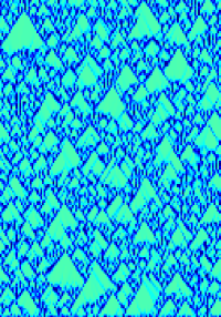
Figure 1: Spatiotemporal evolution of the modulus squared $|A(x,t)|^{2}$ of the scalar CGL equation ($\gamma=0$) for $\alpha=0.2$ and $\beta=-2$. Time is running upwards from $t=0$ to $t=400$ and $x$ is in the horizontal direction. The system size is $L=512$.

Figure 2: Spatiotemporal evolution of $|A_{+}(x,t)|^{2}$ (left) and $|A_{-}(x,t)|^{2}$ (right) for $\gamma=0.7$. The other parameters are as in Fig. 1

When analyzed separately, both $|A_{+}|$ and $|A_{-}|$ display spatiotemporal chaos. The knowledge of one of these variables, however, gives a large amount of information on the other, since they are strongly anticorrelated. This is precisely the content of the concept of generalized synchronization [Kocarev and Parlitz, 1996a, Rulkov et al., 1995]: the two chaotically evolving variables are not identical as in the usual synchronization case, but there is a functional relationship between them which allows close prediction of one of them when the other is known. In [Amengual et al., 1997] the functional relation was identified and a mutual information calculation showed that the generalized synchronization became more perfect as the parameter $\gamma$ approached $\gamma=1$ from below. For $\gamma=1$ the functional relation between the two fields is $|A_{+}|^{2}+|A_{-}|^{2}=1$. The appearance of correlations between the components is clearly mediated by the presence of the localized objects, so that this is a kind of generalized synchronization of chaos specific of spatiotemporal chaos, that is, it is absent in systems without spatial dependence.

It should be noticed that only the moduli $|A_{+}|$ and $|A_{-}|$ develop correlations and we thus find amplitude synchronization. The corresponding phases do not become synchronized. This is the case opposite to the one commonly observed of phase synchronization [Rosenblum et al., 1996]. The reason for this is that the coupling between the fields in Eq. 1 involve only the moduli.

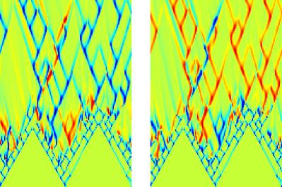
Figure 3: Temporal evolution of $|A_{+}(x,t)|^{2}$ (left) and $|A_{-}(x,t)|^{2}$ (right) starting from an initial condition where $A_{+}(x,0)\approx A_{-}(x,0)$. $\alpha=0.6$, $\beta=-1.4$ and $\gamma=0.7$. The other parameters are as in Fig. 1

Although the meaning and origin of the generalized synchronization found is clear, one often prefers to apply the term “synchronization of chaos” to situations closer to the original ideas [Pecora and Carroll, 1990], which in the present context would mean a tendency of the two fields involved to take identical values, not just anticorrelated ones. We have explored, numerically and analytically, this possibility and found that there exist states in which the amplitude of the two moduli are identical. They are however dynamically unstable, so that the system does not approach them unless particular initial conditions are carefully selected. One example is shown in Fig. 3: during the early part of the evolution the two components are perfectly synchronized, but a decay to the previous anticorrelated case occurs at later times. Further states will be discussed elsewhere. Two types of localized structures can be seen in Fig. 3, the ones for which both fields have simultaneously a hole and the ones in which a hole in one of the fields is associated to a pulse in the other field. Hole-hole and hole-pulse localized structures will also be present in twodimensional systems as we will show in the next section. Furthermore, we will see that topological restrictions can make stable in higher dimensions the hole-hole localized objects related to the ones appearing at the early times in Fig. 3.

3 Twodimensional defects

The onedimensional localized structures of the previous section become topological defects in two dimensions. They have been introduced in [Gil, 1993] and properly classified in [Pismen, 1992, Pismen, 1994]. There are two main types of topological defects in (1): vectorial defects are objects for which the two amplitudes become identical near the defect core, where both vanish. They are the two dimensional analogs of the hole-hole structures present in the early part of Fig. 3. In the other class of defects only one of the amplitudes vanishes, whereas the other presents a maximum. These are the twodimensional analogues of the hole-pulse localized structures in Fig. 2 and in Fig. 3 for larger times. Fig. 4(a) shows the amplitude of one of the two fields containing both types of defects. The vectorial ones emit waves that entrain a whole domain around them whereas defects in which only one amplitudes vanishes behave more passively and remain at the domain borders. In fig. 4(b) the global phase $\phi_{g}=\phi_{+}+\phi_{-}$, where $\phi_{+}$ and $\phi_{-}$ are the phases of $A_{+}$ and $A_{-}$, is plotted. Clearly, there are two different kinds of vectorial defects. One is produced by two defects of the same topological charge, which correspond to the two-armed spiral in the plot of $\phi_{g}$. The other is generated with defects of opposite charges, leading to a target pattern in the plot of $\phi_{g}$.

In the dynamical evolution from random initial conditions, vectorial defects are spontaneously formed for the set of parameters of Fig. 4. This is the same set of parameters explored in [Amengual et al., 1997] for a 1D problem and it leads here to a glassy or frozen configuration like the one shown. However, increasing the value of the coupling parameter $\gamma$, the vectorial defects become unstable. The system evolves then in a disordered dynamics which is governed by defects in which only one amplitudes vanishes. The number of defects is conserved, after a transient regime, during very long times of evolution. A snapshot of this state is shown in Fig 5, where it is seen that a zero of one of the amplitudes corresponds to a maximum of the other one. These defects, strongly anticorrelated in amplitude, move together in time so that the kind of spatiotemporal chaos they sustain displays generalized synchronization between the two amplitudes $|A_{\pm}|$.

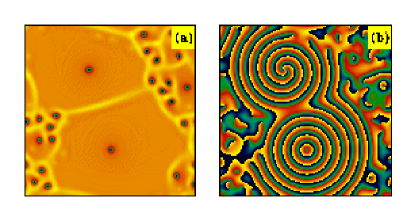
Figure 4: Field configuration showing different kinds of defects in two spacial dimensions. One of the amplitudes, $|A_{+}|^{2}$ (a), and the global phase $\phi_{g}$ (b), at a given time are shown. Parameters used: $\gamma=0.1$, $\alpha=0.2$ and $\beta=2$, system size 128$\times$128.

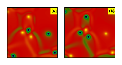
Figure 5: Snapshot of the intensities of the two fields (a) $|A_{+}|^{2}$ and (b) $|A_{-}|^{2}$ for $\gamma=0.8$ and $\alpha$ and $\beta$ as in Fig 4. A dark blue (yellow) dot corresponds to a zero (maximum) of the amplitude.

A quantitative description of the process of increasing generalized synchronization as $\gamma$ is increased can be given in terms of information measures as already introduced for the 1D case in [Amengual et al., 1997]. This description also identifies the transition from glassy to dynamic states due to the instability of the vectorial defects. The joint probability density $p(|A_{+}|,|A_{-}|)$ is plotted in fig. 6 for different values of $\gamma$, as a 3D plot and, in the same figure, as a density plot. The density plot is obtained taking the simultaneous values of $|A_{+}|$ and $|A_{+}|$ at different space-time points. For a small coupling, $\gamma=0.1$, we obtain a diffuse cloud of points with a broad maximum around $|A_{+}|\simeq|A_{-}|\simeq 1$ with deviations from these values being uncorrelated, except for the points laying in the line $|A_{+}|=|A_{-}|$. The presence of such line in plots of coupled variables is the classical signature of conventional synchronization. The points on the line correspond to the core of the vectorial defects in which the two amplitudes take the same value. For $\gamma\simeq 0.3$, the cloud of points broadens and the line $|A_{+}|=|A_{-}|$ becomes diffuse and disappears. This behavior identifies the instability of the vectorial defects. Such instability appears in a narrow range of $\gamma$ and with different mechanisms for the two types of vectorial defects. As the coupling is further increased ($\gamma=0.5$ and 0.95), the cloud of points approaches the curve given by $|A_{+}|^{2}+|A_{-}|^{2}=1$ as in one dimension. This indicates anticorrelation between $A_{+}$ and $A_{-}$ and a generalized amplitude synchronization of the dynamics which increases with $\gamma$. Similar qualitative behavior with $\gamma$ is observed for other values of $\alpha$ and $\beta$ for which a glassy state occurs at $\gamma=0$.

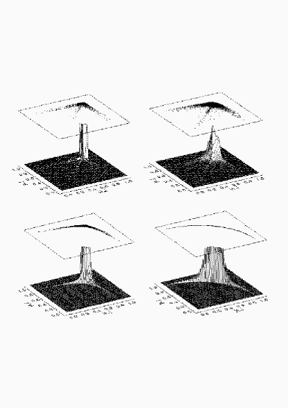
Figure 6: Joint probability distribution $p(|A_{+}|,|A_{-}|)$, for $\alpha$ and $\beta$ as in Fig 4, shown as a 3D surface for different values of $\gamma$. From top to bottom and from left to right, $\gamma=0.1$, 0.3, 0.5 and 0.95. On top of each surface the corresponding plots of $|A_{+}(x,t)|$ vs $|A_{-}(x,t)|$ are shown (the density of dots is proportional to $p(|A_{+}|,|A_{-}|)$). A time average was taken over 100 samples separated $\Delta t=1$. The 3D surfaces for $p(|A_{+}|,|A_{-}|)$ has been cut at $p=0.0025$.

Two quantities that can be extracted from the probability density are the entropy for a single amplitude and their mutual information. The entropy is defined as $H(X)=-\sum_{x}p(x)\ln p(x)$, where $p(x)$ is the probability that $X$ takes the value $x$. $H(X)$ measures the randomness of a discrete random variable $X$. For two random discrete variables $X$ and $Y$, with joint probability density $p(x,y)$, the mutual information $I(X,Y)=-\sum_{x,y}p(x,y)\ln[p(x)p(y)/p(x,y)]$ gives a measure of the statistical dependence between both variables; the mutual information being 0 if and only if $X$ and $Y$ are independent. Considering the discretized values of $|A_{+}|$ and $|A_{-}|$ at space-time points as random variables $X=|A_{+}|$, $Y=|A_{-}|$, their mutual information is a measure of their generalized synchronization. The dependence of the entropy of $A_{+}|$ and $|A_{-}|$ and their mutual information $I$ on the coupling parameter $\gamma$, shown in Fig. 7 identifies three regimes: For low values of $\gamma$ there is a glassy or frozen configuration dominated by large islands around vectorial defects. This relatively ordered state gives a relatively small value of $H$. The mutual information is not large because of the weak coupling between the fields. A second regime is associated with the instability of the vectorial defects. This is highlighted by a maximum value of the entropies and a minimum of $I$ for $\gamma\simeq 0.3$. This instability first disorders the configuration by reducing the size of the domains. This yields an increase of the entropies, but this disorder is not correlated in both components as indicated by the decrease of $I$. For higher values of $\gamma$ ($\gamma>0.35$) we enter the third regime characterized by disordered configurations which evolve in time like the one shown in Fig. 5. The disorder of each amplitude $|A_{\pm}|$ is measured by a relatively large value of $H$, while the increasingly synchronized dynamics is measured by an increasing value of $I$ which approaches its maximum possible value [$I=H(|A_{+}|)=H(|A_{-}|)$] as $\gamma\rightarrow 1^{-}$.

Figure 7: Entropy of $|A_{+}|$ (squares) and $|A_{-}|$ (triangles) and their mutual information $I$ (diamonds) as functions of the coupling parameter $\gamma$ for $\alpha$ and $\beta$ as in Fig 4.

4 Conclusions

We have described generalized synchronization phenomena in the spatiotemporal dynamics of two complex fields which are independent components of a vector complex field. Synchronized dynamics of the amplitudes occurs via localized objects. The motion of these structures produce the dynamical disorder. In $d=1$ localized structures are always dynamical and have the form of anticorrelated pulse-hole structures. Hole-hole type structures are seen to decay after a short transient. In $d=2$ the hole-hole type structures become topological vectorial defects which are stable for small coupling and produce frozen configurations. For coupling above a threshold value these vectorial defects disappear and the persistent dynamics is governed by structures which are topological defects of only one of the fields. These $d=2$ structures show strong amplitude-amplitude anticorrelation and they are the analog of the $d=1$ pulse-hole structures. A quantitative characterization of the degree of synchronization is given by mutual information measures.

5 Acknowledgments

Financial support from DGYCIT Project PB94-1167 (Spain) is acknowledged. R.M. also acknowledges financial support from CONICYT-Fondo Clemente Estable (Uruguay). M.H. also acknowledges financial support from the FOMEC project 290, Dep. de Física FCEyN, Universidad Nacional de Mar del Plata (Argentina).

References

- Amengual et al., 1997 Amengual, A., Hernández-García, E., Montagne, R. and San Miguel, M. [1997] “Synchronization of Spatiotemporal Chaos: The Regime of Coupled Spatiotemporal Intermittency,” Phys. Rev. Lett. 78, 4379-4382.
- Amengual et al., 1996 Amengual, A., Walgraef, D., San Miguel, M., and Hernández-García [1996] “Wave Unlocking Transition in Resonantly Coupled Complex Ginzburg-Landau Equations,” Phys. Rev. Lett. 76, 1956-1959.
- Chaté & Manneville, 1996 Chaté, H. & Manneville, P. [1996] “Phase diagram of the two-dimensional complex Ginzburg-Landau equation,” Physica A 224, 348-368.
- Chaté, 1994a Chaté, H. [1994a] “Spatiotemporal intermittency regimes of the one-dimensional complex Ginzburg-Landau equation,” Nonlinearity 7, 185-204.
- Chaté, 1994b Chaté, H. [1994b] “Disordered regimes of the one-dimensional complex Ginzburg-Landau equation,” in Spatio-Temporal Patterns in Non-equilibrium Complex Systems, eds P.E. Cladis & P. Palffy-Muhoray (Addison-Wesley, Reading, MA).
- Eguiluz et al., 1998 Eguíluz, V.M., Hernández-García, E., & Piro, O. [1998] “Boundary effects in the complex Ginzburg-Landau equation,” This issue.
- Gil, 1993 L. Gil [1993] “Vector Order Parameter for an Unpolarized Laser and its Vectorial Topological Defects,” Phys. Rev. Lett. 70, 162-165.
- Hagan, 1982 Hagan, P.S. [1982] “Spiral waves in reaction-diffusion equations,” SIAM J. Appl. Math 42, 762-786.
- Huygens, 1665 Huygens, C. [1665] J. Scavants XI, 79-80; XII, 86.
- Kocarev and Parlitz, 1996a Kocarev, L. and Parlitz, U. [1996] “Generalized synchronization, predictability, and equivalence of unidirectionally coupled dynamical systems,” Phys. Rev. Lett., 76, 1816-1819.
- Kocarev and Parlitz, 1996b Kocarev, L. and Parlitz, U. [1996] “Synchronizing spatiotemporal chaos in coupled nonlinear oscillators,” Phys. Rev. Lett., 77, 2206-2209.
- Pecora and Carroll, 1990 Pecora, L.M. and Carroll, T.L. [1990], “Synchronization in chaotic systems,” Phys. Rev. Lett. 64, 821.
- Pismen, 1992 Pismen, L. [1992] “On interaction of spiral waves,” Physica D 54, 183-193.
- Pismen, 1994 Pismen, L. [1994] “Energy versus Topology: Competing Defect Structures in 2D Complex Vector Field,” Phys. Rev. Lett. 72, 2557-2560;
- Rosenblum et al., 1996 Rosenblum, M.G., Pikovsky, A.S. and Kurths, J. [1996] “Phase synchronization of chaotic oscillators,” Phys. Rev. Lett. 76, 1804-1807.
- Rulkov et al., 1995 Rulkov, N.F., Sushchik, M.M., Tsimring, T.S. and Abarbanel, H.D.I. [1995] “Generalized synchronization of chaos in directionally coupled chaotic systems,” Phys. Rev. E 51, 980-994.
- San Miguel, 1996 San Miguel, M. [1996] “Phase Instabilities in the Laser Vector Complex Ginzburg Landau Equation,” Phys. Rev. Lett. 75, 425-428.
- Shraiman et al., 1992 Shraiman, B.I., Pumir, A., van Saarlos, W., Hohenberg, P.C, Chaté, H. & Holen, M. [1992] “Spatiotemporal chaos in the one-dimensional Ginzburg-Landau equation,” Physica D 57, 241-248.
- Strogatz and Steward, 1993 Strogatz, S.H. and Steward, I., [1993] “Coupled Oscillators and Biological Synchronization,” Scientific American 269, No. 6, 102.
- van Hecke et al., 1998 van Hecke, M., Storm, C., van Saarloos, W. [1998] “Sources, sinks and wavenumber selection in coupled CGL equations and experimental implications for counter-propagating wave systems,” preprint.
- van Hecke, 1998 van Hecke, M. [1998] “The building blocks of spatiotemporal intermittency,” Phys. Rev. Lett. 80, 1896-1899.
- van Saarloos, 1994 van Saarloos, W. [1994] “The Complex Ginzburg-Landau Equation for Beginners,” in Spatio-Temporal Patterns in Non-equilibrium Complex Systems, eds P.E. Cladis & P. Palffy-Muhoray (Addison-Wesley, Reading, MA).
- Winfree, 1980 Winfree, A.T. [1980] The Geometry of Biological Time, Springer (New York).