Significance of ghost orbit bifurcations in semiclassical spectra

Abstract

Gutzwiller’s trace formula for the semiclassical density of states in a chaotic system diverges near bifurcations of periodic orbits, where it must be replaced with uniform approximations. It is well known that, when applying these approximations, complex predecessors of orbits created in the bifurcation (“ghost orbits”) can produce pronounced signatures in the semiclassical spectra in the vicinity of the bifurcation. It is the purpose of this paper to demonstrate that these ghost orbits themselves can undergo bifurcations, resulting in complex, nongeneric bifurcation scenarios. We do so by studying an example taken from the Diamagnetic Kepler Problem, viz. the period quadrupling of the balloon orbit. By application of normal form theory we construct an analytic description of the complete bifurcation scenario, which is then used to calculate the pertinent uniform approximation. The ghost orbit bifurcation turns out to produce signatures in the semiclassical spectrum in much the same way as a bifurcation of real orbits would.

1 Introduction

Since its discovery in the early 1970s, Gutzwiller’s trace formula [1, 2] has become a widely used tool for the interpretation of quantum mechanical spectra of systems whose classical counterpart exhibits chaotic behaviour. It represents the density of states of the quantum system as a sum over a smooth part and fluctuations from all periodic orbits of the classical system, where the contribution of a single periodic orbit reads

$${\cal A}_{\rm po}=\frac{T_{\rm po}\rme^{\rmi(S_{\rm po}/\hbar-\frac{\pi}{2}\mu_{\rm po})}}{\sqrt{|\det(M_{\rm po}-I)|}}\;,$$ (1)

with $T_{\rm po},S_{\rm po},M_{\rm po},\mu_{\rm po}$ denoting the orbital period, action, monodromy matrix, and Maslov index, respectively. This formula assumes that all periodic orbits can be regarded as isolated, which is the case, in particular, for completely hyperbolic systems. In the generic case of mixed regular-chaotic dynamics, however, the formula fails whenever bifurcations of periodic orbits occur, because close to a bifurcation periodic orbits approach one another arbitrarily closely. The failure of the formula manifests itself in divergences of the periodic orbit contributions (1).

The generic cases of period-$m$-tupling bifurcations were studied by Ozorio de Almeida and Hannay [3, 4], who derived uniform semiclassical approximations by taking into account all orbits involved in a bifurcation collectively. Their solutions were refined by Sieber and Schomerus [5, 6, 7], who derived uniform approximations for all types of bifurcations of codimension one in generic Hamiltonian systems with two degrees of freedom. Their formulas smooth the divergence in Gutzwiller’s trace formula, and, in contrast to the approximations in [3, 4], asymptotically approach the result of the trace formula (1) for isolated periodic orbit contributions as the distance from the bifurcation increases. As a characteristic feature, uniform approximations require the inclusion of complex “ghost orbits”. At the bifurcation points, new periodic orbits are born. However, before they come into being, the orbits possess predecessors – ghost orbits – in the complexified phase space. As was shown by Kuś et al. [8], some of these ghost orbits, which in the limit $\hbar\to 0$ yield exponentially small contributions, have to be included in Gutzwiller’s trace formula (1). As a result, in constructing a uniform approximation complete information about the bifurcation scenario including the ghost orbits is required.

A closer inspection of the bifurcation scenarios encountered in practical applications of uniform approximations reveals that bifurcations of codimension two, although they cannot generically be observed if only one control parameter is varied, can nevertheless have an effect on semiclassical spectra, because in their neighbourhood two bifurcations of codimension one come close to each other, and therefore have to be treated collectively. Examples of that situation have been studied by Main and Wunner [9, 10] as well as Schomerus and Haake [11, 12].

The bifurcation scenarios described in the literature so far involve bifurcations of real orbits only. However, one should expect bifurcations of ghost orbits also to be possible and of particular importance for complicated bifurcation scenarios with codimension greater than one. It is the purpose of this paper to demonstrate that ghost orbit bifurcations do indeed occur and have a pronounced effect on semiclassical spectra. To this end, we present an example taken from the Diamagnetic Kepler Problem. It turns out that even the analysis of the period-quadrupling bifurcation of one of the shortest periodic orbits in that system requires the inclusion of a ghost bifurcation.

The appearance of ghost orbit bifurcations represents an additional challenge for the construction of uniform approximations. It will turn out that normal form theory allows treating both ghost bifurcations and bifurcations of real orbits on an equal footing. Consequently, ghost bifurcations contribute to uniform approximations in much the same way as real bifurcations do. From these observations we conclude that the occurence of ghost bifurcations in systems with mixed regular-chaotic dynamics is not a very exotic but rather quite a common phenomenon.

The organization of the paper is as follows: In section 2 we describe the bifurcation scenario of the example chosen in detail. Section 3 provides the general form of uniform approximations. Section 4 presents the normal form describing the bifurcation scenario in point and the discussion of how the ghost bifurcation can be included in the normal form. In section 5 we determine the normal form parameters to quantitatively describe the bifurcations, and in section 6 the uniform approximation is evaluated.

2 The bifurcation scenario

As an example, we study the hydrogen atom in a magnetic field, which has been described in detail, e.g., in Refs. [13, 14, 15]. We assume the nucleus fixed and regard the electron as a structureless point charge. If the magnetic field is directed along the $z$-axis, the nonrelativistic Hamiltonian describing the electron motion reads [in atomic units, with $\gamma=B/(2.35\times 10^{5}\,{\rm T})$ the magnetic field strength]

$$H=\frac{1}{2}\bi{p}^{2}+\frac{1}{2}\gamma L_{z}+\frac{1}{8}\gamma^{2}\left(x^{2}+y^{2}\right)-\frac{1}{r}=E\;.$$ (2)

Here, $r$ is the distance from the nucleus, and $L_{z}$ denotes the angular momentum along the field axis, which is conserved because of the rotational symmetry around that axis. In the following we restrict ourselves to the case where $L_{z}=0$.

To further simplify the Hamiltonian, we exploit its scaling property with respect to the magnetic field strength $\gamma$. In scaled coordinates and momenta

$$\tilde{\bi{r}}=\gamma^{2/3}\bi{r},\qquad\tilde{\bi{p}}=\gamma^{-1/3}\bi{p}$$ (3)

the Hamiltonian assumes the form

$$\tilde{H}=\gamma^{-2/3}H=\frac{1}{2}\tilde{\bi{p}}^{2}+\frac{1}{8}\left(\tilde{x}^{2}+\tilde{y}^{2}\right)-\frac{1}{\tilde{r}}=\tilde{E}\;.$$ (4)

Thus, the classical dynamics does not depend on the energy $E$ and field strength $\gamma$ separately, but only on the scaled energy $\tilde{E}=\gamma^{-2/3}E$. From the scaling prescriptions (3) and (4) we derive the scaling laws for classical actions and times as

$$\tilde{S}=\gamma^{1/3}S\;,\qquad\tilde{T}=\gamma T\;.$$ (5)

Due to the Coulomb potential, the Hamiltonian (4) is singular at $\tilde{r}=0$. The equations of motion can be regularized by introducing semiparabolical coordinates

$$\mu^{2}=\tilde{r}+\tilde{z}\;,\qquad\nu^{2}=\tilde{r}-\tilde{z}\;,$$ (6)

and a new time parameter $\tau$ defined by $dt=2r\,d\tau$. Finally, the regularized Hamiltonian is obtained as [13, 14, 15]

$${\cal H}=\frac{1}{2}\left(p_{\mu}^{2}+p_{\nu}^{2}\right)-\tilde{E}\left(\mu^{2}+\nu^{2}\right)+\frac{1}{8}\mu^{2}\nu^{2}\left(\mu^{2}+\nu^{2}\right)\equiv 2\;,$$ (7)

and Hamilton’s equations of motion read [with primes denoting derivatives $\rmd/\rmd\tau$],

$$\eqalign{\mu^{\prime}=p_{\mu}\;,&p_{\mu}^{\prime}=2\tilde{E}\mu-\frac{1}{4}\mu\nu^{2}(2\mu^{2}+\nu^{2})\;,\\ \nu^{\prime}=p_{\nu}\;,&p_{\nu}^{\prime}=2\tilde{E}\nu-\frac{1}{4}\mu^{2}\nu(\mu^{2}+2\nu^{2})\;.}$$ (10)

These equations are free of singularities and can easily be integrated numerically. When using them, we must keep in mind that the definition (6) determines the semiparabolical coordinates $\mu,\nu$ up to a choice of sign only, giving a many-to-one coordinate system. Thus, if we integrate the equations of motion (10) until the trajectory closes in $(\mu,\nu)$-coordinates this may correspond to more than one period in the original configuration space. Furthermore, we have to identify orbits which can be transformed into one another by reflections at the coordinate axes.

We now complexify our phase space by allowing coordinates and momenta to assume complex values. This extension allows us to look for ghost predecessors of real orbits born in a bifurcation [9].

At any given scaled energy $\tilde{E}$, there is a periodic orbit along the magnetic field axis. For sufficiently low negative $\tilde{E}$ it is stable, while, as $\tilde{E}\nearrow 0$, it loses and regains stability infinitely often [16, 13]. Stability is lost, for the first time, at $\tilde{E}=-0.391$. At this scaled energy, the so-called balloon orbit [17] is born as a new, stable periodic orbit. As the scaled energy increases further, the orbit exhibits all kinds of period-$m$-tupling bifurcations before finally turning unstable at $\tilde{E}=-0.291$.

Here, we consider the period-quadrupling bifurcation of the balloon orbit at $\tilde{E}_{c}=-0.342025$. For $\tilde{E}>\tilde{E}_{c}$, two real satellite orbits of quadruple period exist. As $\tilde{E}\searrow\tilde{E}_{c}$, they collide with the balloon orbit and form an island-chain bifurcation as described in [3, 4]. The real orbits are shown in figure 1 at scaled energy $\tilde{E}=-0.340$. The solid and dashed curves represent the stable and unstable satellite orbits, respectively. For comparison, the balloon orbit is shown as a dotted curve. Below $\tilde{E}_{c}$, no real satellite orbits exist. Instead, there are a stable and an unstable complex ghost satellite. The real and imaginary parts of the stable and unstable ghost orbits at scaled energy $\tilde{E}=-0.343$ are drawn as solid and dotted curves in figure 2. Note that the imaginary parts are small compared to the real parts. As predicted by normal form theory (see section 4.1), both satellites coincide with their complex conjugates, whence the total number of orbits is conserved in the bifurcation.

The orbits described so far form a generic type of period-quadrupling bifurcation as investigated by Sieber and Schomerus [7]. However, the classical periodic orbit search in the complexified phase space reveals the existence of an additional ghost orbit at scaled energies around $\tilde{E}_{c}$. The shape of this orbit is shown as the dashed curve in figure 2. It is similar to the stable ghost satellite originating from the period-quadrupling of the balloon orbit. When following this ghost orbit to lower energies we find another bifurcation at $\tilde{E}_{c}^{\prime}=-0.343605$, i.e., slightly below the bifurcation point $\tilde{E}_{c}=-0.342025$ of the period-quadrupling of the balloon orbit. At energy $\tilde{E}=\tilde{E}_{c}^{\prime}$ the additional ghost orbit (dashed curve in figure 2) collides with the stable ghost satellite of the period-quadrupling bifurcation (solid curve in figure 2), and these two orbits turn into a pair of complex conjugate ghost orbits. Their shapes are presented at scaled energy $\tilde{E}=-0.344$ by the solid and dashed curves in figure 3. The imaginary parts clearly exhibit the loss of conjugation symmetry described, if the aforementioned symmetry of the semiparabolical coordinate system is taken into account. The dotted curve in figure 3 is the unstable ghost satellite which already exists at higher energy $\tilde{E}>\tilde{E}_{c}^{\prime}$ (see the dotted curve in figure 2).

It is important to note that the second bifurcation at $\tilde{E}=\tilde{E}_{c}^{\prime}$ involves ghost orbits only. This kind of bifurcation has not been described in the literature so far; in particular, Meyer’s classification of codimension-one bifurcations [18] contains bifurcations of real orbits only and does not cover ghost bifurcations. The existence of the ghost orbit bifurcation implies that the results of Ref. [7] for the uniform semiclassical approximation for the generic period-quadrupling bifurcation cannot be applied to the more complicated bifurcation scenario considered here. As in cases described before by Main and Wunner [9, 10] and Schomerus and Haake [11, 12], the closeness of the two bifurcations requires the construction of a uniform approximation taking into account all orbits involved in the successive bifurcations collectively. Thus, the ghost bifurcation at $\tilde{E}_{c}^{\prime}$ turns out to contribute to the semiclassical approximation in the same way as a real bifurcation would, as long as we do not go to the extreme semiclassical domain where the bifurcations can be regarded as isolated. We will demonstrate in section 4 that the techniques of normal form theory can be extended as to include the description of ghost bifurcations.

The construction of the uniform approximation requires the knowledge of the periodic orbit parameters of all orbits participating in the bifurcation scenario. The numerically calculated parameters are shown in figure 4 as functions of the scaled energy $\tilde{E}$. Part (a) of this figure displays the actions of the periodic orbits, where the action of four repetitions of the balloon orbit was chosen as a reference level ($\Delta S=0$). This kind of presentation exhibits the sequence of bifurcations more clearly than a plot of the actual action integrals. Around $\tilde{E}_{c}$, we recognize two almost parabolic curves, indicating the actions of the stable (upper curve) and unstable (lower curve) satellites, respectively. At $\tilde{E}_{c}$, the curves change from solid to dashed as the satellites become complex. Below $\tilde{E}_{c}$, the unstable ghost satellite does not undergo any further bifurcations in the energy range shown, whereas the stable satellite collides, at $\tilde{E}_{c}^{\prime}$, with the additional ghost orbit, which can clearly be seen not to be involved in the bifurcation at $\tilde{E}_{c}$. Below $\tilde{E}_{c}^{\prime}$, these two orbits are complex conjugates of each other. Thus, the real parts of their actions coincide, whereas the imaginary parts are different from zero and have opposite signs.

Analogously, figure 4b displays the orbital periods. Here, no differences were taken, so that the fourth repetition of the balloon orbit, which is always real, shows up as a nearly horizontal solid line at $\tilde{T}\approx 5.84$. The other orbits can be identified with the help of the bifurcations they undergo, in the same way as discussed above. Finally, figure 4c presents the traces of monodromy matrices minus two. These quantities agree with $\det(M-I)$ for systems with two degrees of freedom. At $\tilde{E}_{c}$ and $\tilde{E}_{c}^{\prime}$, they can be seen to vanish for the orbits involved in the bifurcations, causing the divergences of the periodic orbit amplitudes (1) at the bifurcation points.

The generic period-quadrupling bifurcation at $\tilde{E}_{c}$ can be described with the help of lowest order normal form theory presented in section 4.1. As the ghost bifurcation is approached, this description fails. However, the influence of the additional ghost orbit can be taken into account by including higher order terms in the normal form as discussed in section 4.2.

3 The general form of the uniform approximation

Before we return to classical normal form theory in section 4, we introduce, in this section, the basic formulas for the quantum density of states necessary for the construction of the uniform semiclassical approximation. The density of states of a quantum system with the Hamiltonian $\hat{H}$ can be expressed with the help of the Green’s function $G(E)=(E-\hat{H})^{-1}$ as

$$d(E)=-\frac{1}{\pi}{\rm Im}\,\Tr\,G(E)\;,$$ (11)

where the trace of the Green’s function can be evaluated in the coordinate representation,

$$\Tr\,G(E)=\int d\bi{x^{\prime}}d\bi{x}\delta(\bi{x^{\prime}}-\bi{x})G(\bi{x^{\prime}}\bi{x},E)\;.$$ (12)

The basic steps in the formulation of periodic orbit theory [1, 2] are to replace the Green’s function $G(\bi{x^{\prime}}\bi{x},E)$ with its semiclassical Van Vleck-Gutzwiller approximation and to carry out the integrals in stationary-phase approximation. For systems with two degrees of freedom the semiclassical approximation to the Green’s function reads

$$G(\bi{x^{\prime}}\bi{x},E)=\frac{1}{\rmi\hbar\sqrt{2\pi\rmi\hbar}}\sum_{\rm class.~{}traj.}\sqrt{D}\exp\left\{\frac{\rmi}{\hbar}S(\bi{x^{\prime}}\bi{x},E)-\rmi\frac{\pi}{2}\nu\right\}\;.$$ (13)

Here, the sum extends over all classical trajectories running from $\bi{x}$ to $\bi{x^{\prime}}$ at energy $E$, $S$ is the action of a trajectory, $\nu$ its Maslov index, and $D$ is defined by the second derivatives of the action,

$$D=\det\left(\begin{array}[]{cc}\frac{\partial^{2}S}{\partial\bi{x^{\prime}}\partial\bi{x}}&\frac{\partial^{2}S}{\partial\bi{x^{\prime}}\partial E}\\[2.15277pt] \frac{\partial^{2}S}{\partial E\partial\bi{x}}&\frac{\partial^{2}S}{\partial E^{2}}\end{array}\right)\;.$$ (14)

The contribution of a single orbit to the density of states can be evaluated by introducing coordinates parallel and perpendicular to the orbit. The integration along the orbit can then be performed in a straightforward fashion. Finally, Gutzwiller’s trace formula (1) for isolated periodic orbits is obtained by integrating over the coordinates perpendicular to the trajectory using the stationary-phase approximation. It is this last step which fails close to a bifurcation, where periodic orbits are not isolated.

To find an expression for the density of states which is valid close to bifurcations, it is convenient to go over to a coordinate-momentum representation of the Green’s function. Close to a period-$m$-tupling bifurcation of a real orbit the uniform approximation takes the form [5]

$$d(E)=\frac{1}{2\pi^{2}m\hbar^{2}}\,{\rm Re}\,\int dy\,dp_{y}^{\prime}\,\frac{\partial\hat{S}}{\partial E}\sqrt{\left|\frac{\partial^{2}\hat{S}}{\partial y\partial p_{y}^{\prime}}\right|}\exp\left\{\frac{\rmi}{\hbar}\left(\hat{S}+yp_{y}^{\prime}\right)-i\frac{\pi}{2}\hat{\nu}\right\}\;,$$ (15)

with $y$, $p_{y}^{\prime}$, and $\hat{S}$ defined as follows. Let $(y,p_{y})$ be the canonical variables in the Poincaré surface of section perpendicular to the bifurcating orbit, and $(y^{\prime},p_{y}^{\prime})$ the corresponding variables after the period-$m$ cycle of the orbit. The function

$$\hat{S}(p_{y}^{\prime}y,E)=S(y^{\prime}y,E)-y^{\prime}p_{y}^{\prime}$$ (16)

is the Legendre transform of the action integral with respect to the final coordinate or, in other words, the generating function of the Poincaré map for $m$ periods of the bifurcating orbit in a coordinate-momentum representation.

The function in the exponent in (15),

$$f(y,p_{y}^{\prime},E)=\hat{S}(y,p_{y}^{\prime},E)+yp_{y}^{\prime}\;,$$ (17)

is stationary at the fixed points of the $m$-traversal Poincaré map, that is, fixed points of $f$ correspond to classical periodic orbits. In the spirit of catastrophe theory, we now relate $f$ to a given ansatz function $\Phi$, which has the same distribution of stationary points, by a smooth invertible change of coordinates $\psi$ as

$$f(y,p_{y}^{\prime},E)=S_{0}(E)+\Phi(\psi(y,p_{y}^{\prime};E);E)\;.$$ (18)

Here, $\psi$ is assumed to keep the origin fixed, $\psi(0,0;E)=(0,0)$, and $S_{0}(E)$ is the action of the central bifurcating orbit. Inserting this ansatz, we obtain

$$\eqalign{d(E)=\frac{1}{2\pi^{2}m\hbar^{2}}\,{\rm Re}\,\exp\left\{\frac{\rmi}{\hbar}S_{0}(E)-\rmi\frac{\pi}{2}\hat{\nu}\right\}\\ \times\int dY\,dP_{Y}^{\prime}\frac{\partial\hat{S}}{\partial E}\sqrt{\left|\frac{\partial^{2}\hat{S}}{\partial y\partial p_{y}^{\prime}}\right|}\sqrt{\frac{|{\rm Hess}\,\Phi|}{|{\rm Hess}\,f|}}\exp\left\{\frac{\rmi}{\hbar}\Phi(Y,P_{Y}^{\prime})\right\}\;,}$$ (21)

where ${\rm Hess}\,$ denotes the Hessian matrix and the coefficient

$$X:=\frac{\partial\hat{S}}{\partial E}\sqrt{\left|\frac{\partial^{2}\hat{S}}{\partial y\partial p_{y}^{\prime}}\right|}\sqrt{\frac{|{\rm Hess}\,\Phi|}{|{\rm Hess}\,f|}}$$ (22)

is unknown. At a stationary point of $\Phi$, it can be shown to assume the value

$$X\stackrel{{\scriptstyle sp}}{{=}}\frac{\{m\}T}{\sqrt{|\Tr M-2|}}\sqrt{|{\rm Hess}\,\Phi|}\;,$$ (23)

where $T$ and $M$ denote the period and the monodromy matrix of the corresponding classical orbit, and the notation $\{m\}$ is meant to indicate that this factor does not occur at the satellite orbits.

4 Normal-form description of the bifurcation

To evaluate the uniform approximation (21), we need to find a suitable ansatz function $\Phi$. Normal form theory as developed by Birkhoff [19] and Gustavson [20] provides us with a systematic way to construct such ansatz functions. We will first investigate the lowest nontrivial order of the normal form expansion which describes generic bifurcations. Then, we will show that higher-order terms in the expansion can account for the more complicated bifurcation scenario studied here.

4.1 The generic period-quadrupling bifurcation

The simplest normal form describing the generic period-quadrupling bifurcations reads [3]

$$\Phi=\varepsilon I+aI^{2}+bI^{2}\cos(4\varphi)\;.$$ (24)

This normal form is expressed in terms of canonical (action-angle) polar coordinates $(I,\varphi)$, which are connected to Cartesian coordinates $(p,q)$ by

$$p=\sqrt{2I}\cos\varphi\;,\qquad q=\sqrt{2I}\sin\varphi\;.$$ (25)

To establish the connection with classical periodic orbits, we need to determine the stationary points of the normal form and then evaluate its stationary values. The stationary points are given by the equations

$$\eqalign{0&\stackrel{{\scriptstyle\textstyle!}}{{=}}\frac{\partial\Phi}{\partial\varphi}=-4I^{2}b\sin(4\varphi)\;,\\ 0&\stackrel{{\scriptstyle\textstyle!}}{{=}}\frac{\partial\Phi}{\partial I}=\varepsilon+2aI+2bI\cos(4\varphi)\;.}$$ (28)

The first of these equations yields

$$\eqalign{\sin(4\varphi)=0\;,\\ \cos(4\varphi)=\sigma=\pm 1\;,}$$ (31)

so that the second equation reads

$$\varepsilon+2(a+\sigma b)I=0\;,$$

with its solution

$$I_{\sigma}=-\frac{\varepsilon}{2(a+\sigma b)}\;.$$ (32)

In addition, there is the central periodic orbit at $I=0$, which does not show up as a stationary point because the polar coordinate system (25) is singular at the origin.

To interprete these results, we observe that according to its definition (25) the coordinate $I$ is positive for real orbits and that the action difference $\Phi(I,\varphi)$ is real for real $I,\varphi$. Therefore, negative real solutions $I$ correspond to ghost orbits which are symmetric with respect to complex conjugation and thus have real actions, whereas a complex $I$ indicates an asymmetric ghost orbit.

Now, if $|a|>|b|$, the two solutions $I_{\pm}$ have the same sign, which changes at $\varepsilon=0$. So, the two satellite orbits change from two real orbits to two ghosts at the bifurcation point $\varepsilon=0$, forming an island-chain-bifurcation. If $|a|<|b|$, $I_{+}$ and $I_{-}$ have different signs, so that on either side of the bifurcation there is one real and one ghost satellite. At $\varepsilon=0$, the satellites collide with the central orbit, forming a touch-and-go-bifurcation.

4.2 Generalization to nongeneric bifurcations

To describe a sequence of two bifurcations, we need to include higher-order terms in the normal form. Here, we adopt the normal form

$$\Phi=\varepsilon I+aI^{2}+bI^{2}\cos(4\varphi)+cI^{3}(1+\cos(4\varphi))$$ (33)

given by Schomerus [21] as a variant of the normal form used by Sadovskií and Delos [22] to describe a sequence of bifurcations close to a period-quadrupling. It turns out to qualitatively describe the sequence of bifurcations encountered here for suitably chosen parameter values.

The stationary points of $\Phi(I,\varphi)$ are given by the equations

$$\eqalign{0&\stackrel{{\scriptstyle\textstyle!}}{{=}}\frac{\partial\Phi}{\partial\varphi}=-4I^{2}(b+cI)\sin(4\varphi)\;,\\ 0&\stackrel{{\scriptstyle\textstyle!}}{{=}}\frac{\partial\Phi}{\partial I}=\varepsilon+2aI+2bI\cos(4\varphi)+3cI^{2}(1+\cos(4\varphi))\;.}$$ (36)

As in section 4.1, the first of these equations yields (see eq. 31)

$$\sin(4\varphi)=0\;,$$

$$\cos(4\varphi)=\sigma=\pm 1\;.$$

Thus, the second equation reads

$$\varepsilon+2(a+\sigma b)I+3cI^{2}(1+\sigma)=0\;.$$ (37)

In solving this equation, we shall assume $c<0$.

For $\sigma=-1$, the equation is linear. Its only solution reads

$$I_{-1}=-\frac{\varepsilon}{2(a-b)}\;.$$ (38)

For $\sigma=+1$, however, we obtain a quadratic equation with two solutions:

$$I_{\pm}=-c^{-1/3}\left(\delta\pm\sqrt{\eta+\delta^{2}}\right)\;,$$ (39)

where we have introduced the abbreviations

$$\eta\equiv-\frac{\varepsilon}{6c^{1/3}},\quad\delta\equiv\frac{a+b}{6c^{2/3}}\;.$$ (40)

Thus, we obtain three different stationary points corresponding to the three satellite orbits in addition to the central periodic orbit at $I=0$.

The dependence of the solutions $I$ on $\varepsilon$ is shown schematically in figure 5 for the case $|a|>|b|$ and $c<0$. Comparing the normal form results to the bifurcation scenario described in section 2, we recognize the sequence of an island-chain-bifurcation at $\varepsilon=0$ and a ghost orbit bifurcation at some negative value of $\varepsilon$. Thus, our normal form correctly describes the bifurcation scenario under consideration, and we adopt it as an ansatz function in the uniform approximation (21). This correspondence allows us to identify stationary points with classical periodic orbits as follows: The $(\sigma=-1)$-solution describes the unstable satellite orbits on either side of $\tilde{E}_{c}$. For $\tilde{E}<\tilde{E}_{c}^{\prime}$, the $(\sigma=+1)$-solutions correspond to the asymmetric ghost orbits, whereas for $\tilde{E}>\tilde{E}_{c}^{\prime}$, we identify the two solutions for $\sigma=+1$ with the stable satellite orbit (marked by the $+$ in figure 5) and with the additional ghost ($-$ in figure 5).

We now calculate the stationary values of the normal form, which correspond to action differences. They read

$$\eqalign{\Phi_{\pm}=4\left(\eta+\delta^{2}\right)\left(\delta\pm\sqrt{\eta+\delta^{2}}\right)+2\eta\delta\;,\\ \Phi_{-1}=-\frac{\varepsilon^{2}}{4(a-b)}\;.}$$ (43)

Finally, we need the Hessian determinants of the normal form at the stationary points. We calculate them with respect to cartesian coordinates, because in polar coordinates the Hessian determinant at the central orbit $I=0$ is undefined, and obtain

$$\eqalign{{\rm Hess}\,_{\pm}=\left\{\varepsilon+2(a-3b)I_{\pm}-2cI_{\pm}^{2}\right\}\left\{\varepsilon+6(a-b)I_{\pm}+30cI_{\pm}^{2}\right\}\;,\\ {\rm Hess}\,_{-1}=\left\{\varepsilon+4aI_{-1}+4cI_{-1}^{2}\right\}^{2}-4I_{-1}^{2}\left\{a-3b-2cI_{-1}\right\}^{2}\;,\\ {\rm Hess}\,_{0}=\varepsilon^{2}\;.}$$ (47)

We have now found a normal form which can serve as an analytical description of the complicated bifurcation scenario.

5 Determination of normal form parameters

In order to use the normal form (33) as an ansatz in the uniform approximation (21), we now have to determine the normal form parameters $\varepsilon,a,b,c$ so that the numerically observed action differences are quantitatively reproduced by the normal form results (43). Since, according to figure 5, $\varepsilon$ measures the distance from the period quadrupling bifurcation, we choose

$$\varepsilon=\tilde{E}-\tilde{E}_{c}\;,$$ (48)

and then solve equations (43) for the parameters $a,b,c$.

To achieve this, we introduce

$$\eqalign{h_{+}&=\frac{\Phi_{+}+\Phi_{-}}{8}=\delta\left(\eta+\delta^{2}\right)+\frac{1}{2}\eta\delta\;,\\ h_{-}&=\frac{\Phi_{+}-\Phi_{-}}{8}=(\eta+\delta^{2})^{3/2}\;.}$$ (51)

The second equation gives

$$\eta=h_{-}^{2/3}-\delta^{2}\;,$$ (52)

so that from the first equation we obtain

$$\delta^{3}-3h_{-}^{2/3}\delta+2h_{+}=0\;.$$ (53)

This is a cubic equation for $\delta$. Its discriminant reads

$$D=h_{+}^{2}-h_{-}^{2}=\frac{1}{16}\Phi_{+}\Phi_{-}\;,$$ (54)

and, using Cardani’s formula, we find its solutions

$$\delta=\frac{\lambda}{2}\sqrt[3]{-\left(\sqrt{\Phi_{+}}+\sqrt{\Phi_{-}}\right)^{2}}+\frac{\lambda^{\ast}}{2}\sqrt[3]{-\left(\sqrt{\Phi_{+}}-\sqrt{\Phi_{-}}\right)^{2}}\;,$$ (55)

where $\lambda\in\left\{1,-\frac{1}{2}\pm\rmi\frac{\sqrt{3}}{2}\right\}$ is a cube root of unity. If $D>0$, $\lambda=1$ yields the only real solution, whereas for $D<0$ all solutions are real. To proceed, we have to choose one of the three solutions.

As can be seen from figure 4 using the correspondence between stationary points and periodic orbits discussed above, we have $\Phi_{+}>0$, and there is an $\varepsilon_{0}<0$ such that $\Phi_{-}>0$ for $\varepsilon>\varepsilon_{0}$ and $\Phi_{-}<0$ for $\varepsilon<\varepsilon_{0}$. Consequently, $D>0$ for $\varepsilon>\varepsilon_{0}$ and $D<0$ for $\varepsilon<\varepsilon_{0}$. To make $\delta$ real, we therefore have to choose $\lambda=1$ if $\varepsilon<\varepsilon_{0}$.

To determine $\lambda$ for $\varepsilon>\varepsilon_{0}$, we first observe that the parameters must depend on $\varepsilon$ continuously. Thus, $\lambda$ can only change at energies where equation (53) has a double root, viz. $D=0$ or $\varepsilon\in\{0,\varepsilon_{0}\}$. Therefore, it suffices to determine $\lambda$ in a neighbourhood of $\varepsilon=0$.

From the plot of action differences in figure 4 we find

$$\Phi_{+}=\alpha^{2}\varepsilon^{2}+\Or\left(\varepsilon^{3}\right)\;,$$

$$\Phi_{-}=-\Gamma-\beta\varepsilon+\Or\left(\varepsilon^{3}\right)\;,$$

with positive constants $\alpha,\beta,\Gamma$. With the help of equations (55) and (52) we can now expand $\eta$ in a Taylor series to first order in $\varepsilon$:

$$\eta=\left(\frac{1}{4}-({\rm Re}\,\lambda)^{2}\right)\Gamma^{2/3}$$

$$+\left(\left(\frac{1}{4}-({\rm Re}\,\lambda)^{2}\right)\frac{2\beta}{3\Gamma^{2/3}}-{\rm Re}\,\lambda\,{\rm Im}\,\lambda\frac{4\alpha\sqrt{\Gamma}}{3\Gamma^{1/3}}{\rm sign}\,\varepsilon\right)\varepsilon+\Or\left(\varepsilon^{2}\right)\;.$$ (56)

Requiring this result to reproduce the definition

$$\eta=-\frac{1}{6c^{1/3}}\varepsilon\;,\qquad-\frac{1}{6c^{1/3}}>0\;,$$

we find the conditions

$${\rm Re}\,\lambda=-\frac{1}{2}\;,\qquad{\rm Im}\,\lambda\frac{2\alpha\sqrt{\Gamma}}{3\Gamma^{1/3}}{\rm sign}\,\varepsilon>0\;,$$

which lead to the correct choices of $\lambda$:

$$\lambda=\cases{1&: $\Phi_{-}>0$\\ -\frac{1}{2}+\rmi\frac{\sqrt{3}}{2}{\rm sign}\,\varepsilon&: $\Phi_{-}<0$}\;.$$ (57)

Using this result, we can determine $\eta$ and $\delta$ from (52) and (55). Equations (40) and (43) then finally yield the desired parameter values

$$\eqalign{c=-\left(\frac{\varepsilon}{6\eta}\right)^{3}\;,\\ a=3c^{2/3}\delta-\frac{\varepsilon}{8\Phi_{-1}}\;,\qquad b=3c^{2/3}\delta+\frac{\varepsilon}{8\Phi_{-1}}\;.}$$ (60)

Note that from (60) the parameters $a$, $b$, and $c$ are explicitly determined as functions of the energy $\varepsilon$ and the three action differences $\Phi_{+}$, $\Phi_{-}$, and $\Phi_{-1}$.

In our case, we will determine the normal form coefficients from the scaled action differences shown in figure 4. To obtain the actual non-scaled coefficients for different values of the magnetic field strength $\gamma$, we need to derive scaling laws for the coefficients. As we shall display the semiclassical spectra as functions of scaled energy, we prefer not to scale the energy difference $\varepsilon=\tilde{E}-\tilde{E}_{c}$. Then, with the help of equations (43) and (47), we can convince ourselves that the scaling prescriptions

$$\tilde{a}=\gamma^{-1/3}a\;,\qquad\tilde{b}=\gamma^{-1/3}b\;,\qquad\tilde{c}=\gamma^{-2/3}c$$ (61)

fulfil the requirements of scaling actions according to $\tilde{S}=\gamma^{1/3}S$ while not scaling Hessian determinants.

6 Evaluation of the uniform approximation

Now that the ansatz function $\Phi$ has been completely specified, a suitable approximation to the coefficient $X$ in (21) remains to be found. We assume $X$ to be independent of $\varphi$, and as the value of $X$ is known at the stationary points of $f$ at four different values of $I$ (including $I=0$), we approximate $X$ by the third order polynomial $p(I)$ interpolating between the four given points. This choice ensures that our approximation reproduces Gutzwiller’s isolated-orbits formula if, sufficiently far away from the bifurcations, we evaluate the integral in stationary-phase-approximation. Thus, the uniform approximation takes its final form

$$d(E)=\frac{1}{2\pi^{2}m\hbar^{2}}\,{\rm Re}\,\exp\left\{\frac{\rmi}{\hbar}S_{0}(E)-\rmi\frac{\pi}{2}\hat{\nu}\right\}\int dY\,dP_{Y}^{\prime}\,p(I)\exp\left\{\frac{\rmi}{\hbar}\Phi(Y,P_{Y}^{\prime})\right\}\;,$$ (62)

which contains known functions only and can be evaluated numerically.

It is important to point out, at this juncture, the progress encorporated in equation (62) as compared to previous literature results. Starting from the lowest-order normal form (24), Sieber and Schomerus [7] derived a similar formula for the contribution of an isolated generic period-quadrupling bifurcation to the density of states. However, as we have seen in section 4.1, their normal form (24) describes the central periodic orbit and the stable and unstable satellites only, from which it is evident that the uniform approximation given by Sieber and Schomerus cannot take the presence of the additional ghost orbit and the occurence of the ghost orbit bifurcation into account. The effect of the latter is negligible far above the bifurcation energy $\tilde{E}_{c}$, where the asymptotic behaviour is determined by the three real orbits common to both (Sieber and Schomerus’s and our own) forms of the uniform approximation. The Sieber and Schomerus result, however, is not capable of describing the correct asymptotic behaviour below $\tilde{E}_{c}$, because one of the satellite orbits runs into a bifurcation unforeseen by the normal form (24) at $\tilde{E}_{c}^{\prime}$, thus causing Sieber and Schomerus’s uniform approximation to diverge. Below $\tilde{E}_{c}^{\prime}$, when the stable satellite orbit does not exist any more, their solution also ceases to exist because the required input data is no longer available. Thus, to obtain a smooth interpolation between the asymptotic Gutzwiller behaviour on either side of the bifurcations, we must make use of the extended uniform approximation (62), which takes the contribution of the ghost orbit bifurcation into account, as long as we do not go to the extreme semiclassical domain where Planck’s constant has become so small that below $\tilde{E}_{c}$ the asymptotic regime is reached before the ghost orbit bifurcation can produce a palpable effect. It is only in this limit that the impact of the ghost orbit bifurcation on the semiclassical spectrum vanishes.

We calculated the uniform approximation (62) for three different values of the magnetic field strength $\gamma$. The results are shown in figure 6. To suppress the highly oscillatory contributions originating from the factor $\exp\left\{\frac{\rmi}{\hbar}S_{0}(E)\right\}$, we plot the absolute value of (62) instead of the real part. As can be seen, the uniform approximation proposed is finite at the bifurcation energies, and, as the distance from the bifurcations increases, asymptotically goes over into the results of Gutzwiller’s trace formula. Even the complicated oscillatory structures in the density of states caused by interferences between the contributions from the different real orbits involved at $\tilde{E}>\tilde{E}_{c}=-0.342025$ are perfectly reproduced by our uniform approximation (see figures 6b and 6c). We also see that the higher the magnetic field strength, the farther away from the bifurcation the asymptotic (Gutzwiller) behaviour is acquired. In fact, for the largest field strength in figure 6a ($\gamma=10^{-10}$) the asymptotic region is not reached at all in the energy domain shown. The magnetic field dependence of the transition into the asymptotic regime can be traced back to the fact that, due to the scaling properties of our system, the scaling parameter $\gamma^{1/3}$ plays the rôle of an effective Planck’s constant, therefore the lower $\gamma$ becomes, the more accurate the semiclassical approximation will be.

7 Conclusion

We have shown that in Hamiltonian systems with mixed regular-chaotic dynamics ghost orbit bifurcations can occur besides the bifurcations of real orbits. These are of special importance when they appear in the vicinity of bifurcations of real orbits, since they turn out to produce signatures in the semiclassical spectra much the same as those of the real orbits. Consequently, the traditional theory of uniform approximations for bifurcations of real orbits must be extended to also include the effects of bifurcating ghost orbits.

We have illustrated the phenomenon of bifurcating ghost orbits in the neighbourhood of bifurcations of real orbits by way of example for the period-quadrupling of the balloon orbit in the diamagnetic Kepler problem, and have demonstrated how normal form theory can be extended for this case so as to allow the unified description of both real and complex bifurcations.

We picked the example mainly for its simplicity, since (a) the real orbit considered is one of the shortest fundamental periodic orbits in the diamagnetic Kepler problem and (b) the period-quadrupling is the lowest period-$m$-tupling possible ($m=4$) that exhibits the island-chain-bifurcation typical of all higher $m$. Thus we expect ghost orbit bifurcations to appear also for longer-period orbits, and, in particular, in the vicinity of all higher period-$m$-tupling bifurcations of real orbits.

In fact, a general discussion of the bifurcation scenarios described by the normal form (33) and its more general variant given in [22] for different values of the parameters leads us to the conclusion that the appearance of ghost bifurcations in the vicinity of bifurcating real orbits is the rule, rather than the exception, in general systems with mixed regular-chaotic systems, and thus one of their generic features. It will be interesting and rewarding to study higher period-$m$-tuplings with respect to the appearance of ghost orbit bifurcations, and to extend ordinary normal form theory to also include the contributions of ghost orbit bifurcations for all higher $m$.

References

Figure 1: Real orbits at scaled energy $\tilde{E}=-0.340>\tilde{E}_{c}$ drawn in scaled semiparabolical coordinates $(\mu=\gamma^{1/3}(r+z)^{1/2},\nu=\gamma^{1/3}(r-z)^{1/2})$. Solid and dashed lines: Stable and unstable satellites created at the period-quadrupling bifurcation of the balloon orbit. Dotted line: Balloon orbit.

Figure 2: Real and imaginary parts of complex ghost orbits at scaled energy $\tilde{E}=-0.343$. Solid and dotted lines: Stable and unstable ghost satellites created at the period-quadrupling bifurcation of the balloon orbit at $\tilde{E}_{c}=-0.342025$. Dashed line: Additional ghost orbit created at the ghost bifurcation at $\tilde{E}_{c}^{\prime}=-0.343605$.

Figure 3: Ghost orbits at scaled energy $\tilde{E}=-0.344<\tilde{E}_{c}^{\prime}$. Solid and dashed lines: Asymmetric ghosts (real parts coincide) created at the ghost bifurcation at $\tilde{E}_{c}^{\prime}=-0.343605$. Dotted line: Unstable ghost satellite created at the period-quadrupling bifurcation of the balloon orbit at $\tilde{E}_{c}=-0.342025$.

Figure 4: Actions, periods and traces of the orbits involved in the bifurcations as functions of the scaled energy $\tilde{E}=E\gamma^{-2/3}$. Solid lines: real orbits, dashed lines: ghost orbits symmetric with respect to complex conjugation, dotted lines: asymmetric ghost orbits.

Figure 5: Sketch of the bifurcation scenario given by the normal form (33) for the case $|a|>|b|$ and $c<0$. Solid lines: Real orbits. Dashed lines: Ghost orbits symmetric with respect to complex conjugation. Dotted line: A pair of complex conjugate ghosts.

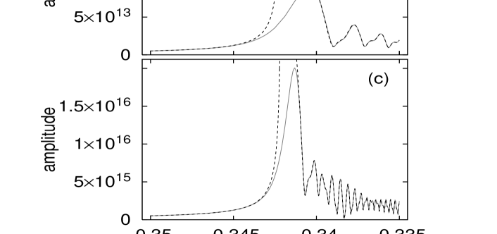
Figure 6: Uniform approximation to the contribution of the considered bifurcations to the density of states for three different values of the magnetic field strength: (a) $\gamma=10^{-10}$, (b) $\gamma=10^{-12}$, (c) $\gamma=10^{-14}$. Solid lines: Uniform approximations. Dashed lines: Gutzwiller’s trace formula.

References

- [1] Gutzwiller M C 1967 J. Math. Phys. 8 1979 and 1971 J. Math. Phys. 12 343
- [2] Gutzwiller M 1990 Chaos in Classical and Quantum Mechanics (New York: Springer)
- [3] Ozorio de Almeida A M and Hannay J H 1987 J. Phys. A 20 5873
- [4] Ozorio de Almeida A M 1988 Hamiltonian Systems: Chaos and Quantization (Cambridge University Press)
- [5] Sieber M 1996 J. Phys. A 29 4715
- [6] Schomerus H and Sieber M 1997 J. Phys. A 30 4537
- [7] Sieber M and Schomerus H 1998 J. Phys. A 31 165
- [8] Kuś M, Haake F, and Delande D 1993 Phys. Rev. Lett. 71 2167
- [9] Main J and Wunner G 1997 Phys. Rev. A 55 1743
- [10] Main J and Wunner G 1998 Phys. Rev. E 57 7325
- [11] Schomerus H 1997 Europhys. Lett. 38 423
- [12] Schomerus H and Haake F 1997 Phys. Rev. Lett. 79 1022
- [13] Friedrich H and Wintgen D 1989 Phys. Rep. 183 37
- [14] Hasegawa H, Robnik M, and Wunner G 1989 Prog. Theor. Phys. Suppl. 98 198
- [15] Watanabe S 1993 in Review of Fundamental Processes and Applications of Atoms and Ions, ed. C. D. Lin (Singapore: World Scientific)
- [16] Wintgen D 1987 J. Phys. B 20 L511
- [17] Mao J M and Delos J B 1992 Phys. Rev. A 45 1746
- [18] Meyer K R 1970 Trans. AMS 149 95
-
[19]
Birkhoff G D 1927, 1966 Dynamical Systems
(Providence, RI: AMS Colloquium Publications vol. IX) - [20] Gustavson F 1966 Astron. J. 71 670
- [21] Schomerus H 1998 J. Phys. A 31 4167
- [22] Sadovskií D A and Delos J B 1996 Phys. Rev. E 54 2033