The Effect of Radiation on the Stochastic Web

Abstract

A charged particle circling in a uniform magnetic field and kicked by an electric field is considered. Under the assumption of small magnetic field, an iterative map is developed. Comparison between the (relativistic) non-radiative case and the (relativistic) radiative case shows that in both cases one can observe a stochastic web structure, and that both cases are qualitatively similar.

]

I Introduction

Zaslavskii et al [1] studied the behavior of particles in the wave packet of an electric field in the presence of a static magnetic field. For a broad wave packet with sufficiently uniform spectrum, one may show that the problem can be stated in terms of an electrically kicked harmonic oscillator. For rational ratios between the frequency of the kicking field and Larmor frequency associated with the magnetic field the phase space of the system is covered by a mesh of finite thickness; inside the filaments of the mesh, the dynamics of the particle is stochastic and outside (in the cells of stability), the dynamics is regular. This structure is called a stochastic web. It was found that this pattern covers the entire phase plane, permitting the particle to diffuse arbitrarily far into the region of high energies (a process analogous to Arnol’d diffusion [2]).

Since the stochastic web leads to unbounded energies, several authors have considered the corresponding relativistic problem. Longcope and Sudan [3] studied this system (in effectively $1\frac{1}{2}$ dimensions) and found that for initial conditions close to the origin of the phase space there is a stochastic web, which is bounded in energy, of a form quite similar, in the neighborhood of the origin, to the non-relativistic case treated by Zaslavskii et al. Karimabadi and Angelopoulos [4] studied the case of an obliquely propagating wave, and showed that under certain conditions, particles can be accelerated to unlimited energy through an Arnol’d diffusion in two dimensions. Since an accelerated charged particle radiates, it is important to study the radiative corrections to this motion. We shall use the Lorentz-Dirac equation to compute this effect.

We compute solutions to this equation for the case of the kicked oscillator. At low velocities, the stochastic web found by Zaslavskii et al[1] occurs; the system diffuses in the stochastic region to unbounded energy, as found by Karimabadi and Angelopoulos[4]. The velocity of the particle is light speed limited by the dynamical equations, in particular, by the suppression of the action of the electric field at velocities approaching the velocity of light [5].

II Model

In the present study we will consider a charged particle moving in a uniform magnetic field, and kicked by an electric field. The effect of relativity, as well as the radiation of the particle, will be considered. We restrict ourselves to the “on mass shell” case.

The fundamental equation that we use to study radiation is the Lorentz-Dirac equation [7], is

$$m_{0}\ddot{x}^{\mu}={e\over c}\dot{x}_{\nu}F^{\mu\nu}+\gamma_{0}m_{0}({\stackrel{{\scriptstyle\dots}}{{x}}^{\mu}}-{1\over c^{2}}\dot{x}^{\mu}\ddot{x}_{\nu}\ddot{x}^{\nu}),$$ (1)

where $\gamma_{0}={2\over 3}{r_{0}\over c}=6.26\times 10^{-24}\sec$. $\mu$ and $\nu$ are the coordinates $t$ and $x$, $y$, and $z$ (or 0, 1, 2, 3), and the derivative is with respect to $\tau$, which can be regarded as proper time in the “on-mass-shell” case. $F^{\mu\nu}$ is the antisymmetric electromagnetic tensor. The first term of the right hand side of Eq. (1) is the relativistic Lorentz force, while the second term is the radiation-reaction term. Note that the small size of the radiation coefficient ($\gamma_{0}\ll 1$) leads to a singular equation that requires special mathematical treatment, as well as physical restrictions, as will be shown in the succeeding sections.

Following Zaslavskii et al [1], the magnetic field is chosen to be a uniform field in the $z$ direction, and the kicking electric field is a function of $x$ in the $x$ direction,

$$\vec{B} = (0,0,B_{0})$$ (2)

$$\vec{E}(x,t) = ({f(x){\sum_{n=-\infty}^{\infty}\delta(t-nT)}},0,0).$$ (3)

Originally, Zaslavskii et al chose a uniform broad band electric field wave packet which can be expanded as an infinite sum of (kicking) $\delta$-functions ($\omega_{0}$ is the frequency of the central harmonic of the wave packet, $k_{0}$ is the wave number of the central harmonic, and $\Delta\omega$ is the frequency between the harmonics of the wave packet)

$$E_{x}=E(x,t)=-E_{0}\sum_{n=-\infty}^{\infty}\sin(k_{0}x-\omega_{0}t-n\Delta\omega t),$$ (4)

which, for $\omega_{0}=0$, becomes

$$E(x,t)=-E_{0}T\sin(k_{0}x)\sum_{n=-\infty}^{\infty}\delta(t-nT),$$ (5)

where $T={{2\pi}\over{\Delta\omega}}$. Eq. (2) is the generalization of Eq. (5), with an arbitrary function $f(x)$ instead of the sine function of Eq. (5).

In order to introduce a map which connects between cycles of integration which start before a kick and end before the next electric field kick, one has first to integrate over the $\delta$ electric kick and then to integrate the equations of motion between the kicks, where only a uniform magnetic field is present and there is no electric field up to the beginning of the next kick.

III The motion of a charged particle in a uniform magnetic field

In the case of a uniform magnetic field from Eq. (2), Eqs. (1) reduce to three coupled differential equations,

$$c\ddot{t} =\ddot{x}_{0}= \gamma_{0}({\stackrel{{\scriptstyle\dots}}{{x}}_{0}}-{1\over{c^{2}}}\dot{x}_{0}R)$$ (6)

$$\ddot{x} =\ddot{x}_{1}= -\Omega\dot{x}_{2}+\gamma_{0}({\stackrel{{\scriptstyle\dots}}{{x}}_{1}}-{1\over{c^{2}}}\dot{x}_{1}R)$$ (7)

$$\ddot{y} =\ddot{x}_{2}= \Omega\dot{x}_{1}+\gamma_{0}({\stackrel{{\scriptstyle\dots}}{{x}}_{2}}-{1\over{c^{2}}}\dot{x}_{2}R),$$ (8)

where $\Omega={{e_{0}B_{0}}\over{m_{0}c}}$, $R=\ddot{x}_{1}^{2}+\ddot{x}_{2}^{2}-\ddot{x}_{0}^{2}$, and $e_{0}=-e$ (charge of the electron).

Using a complex coordinate[8], $u=x+iy$, Eqs. (6) can be written as,

$$\ddot{t} = \gamma_{0}({\stackrel{{\scriptstyle\dots}}{{t}}}-{1\over{c^{2}}}\dot{t}R)$$ (9)

$$\ddot{u} = i\Omega\dot{u}+\gamma_{0}({\stackrel{{\scriptstyle\dots}}{{u}}}-{1\over{c^{2}}}\dot{u}R).$$ (10)

We wish here to constrain the radiatively perturbed motion to the “mass shell”; to do this, it is very convenient to use hyperbolic coordinates,

$$\dot{t} = \cosh q$$ (11)

$$\dot{x} = c\sinh q\cos\phi$$ (12)

$$\dot{y} = c\sinh q\sin\phi$$ (13)

since the “on mass shell” restriction (see [6] for further discussion),

$$\dot{x}^{\mu}\dot{x}_{\mu}=\dot{x}^{2}+\dot{y}^{2}-c^{2}\dot{t}^{2}=-c^{2},$$ (14)

is then automatically satisfied. The complex coordinate $u$ then becomes,

$$\dot{u}=c\sinh qe^{i\phi}$$ (15)

and the equations of motion Eqs. (9) can be written as,

$$\dot{q} = -\gamma_{0}\dot{\phi}^{2}\cosh q\sinh q+\gamma_{0}\ddot{q}$$ (16)

$$\dot{\phi} = \Omega+2\gamma_{0}\dot{\phi}\dot{q}\coth q+\gamma_{0}\ddot{\phi}.$$ (17)

As pointed out earlier, in the case of a singular equation (such as Eqs. (16) and (17)), one has to consider physical arguments as well as mathematical arguments. There are several suggested methods to avoid the “run away electron” problem [7]. One of the most frequently used, especially useful for scattering problems, assumes [9] that the particle loses all its energy after a sufficiently large time, and the run away parts of the solution are set to zero; the equations of motion can then be written as an integral equation. Another method, which permits the study of problems with only non-asymptotic states [10], uses an iterative singular perturbation integration that leads to the stable solution. Since the integration we must use is over a finite time, it is impossible to use an asymptotic condition (e.g. $|v|\to 0$ at $\tau\to\infty$). The Sokolov and Ternov approach [8] is more suitable for our purpose, since it can be implemented for bounded time integration, and the mathematical solution is simple. In this method, in the first step, the perturbation terms in Eq. (17) are disregarded (as in the iterative scheme of [10]) , and then the resulting equation is exactly integrated. In the second step, the singular term on the right hand side of Eq. (16) is not considered; using $\phi(\tau)$ from Eq. (17), the equation including just the first term is integrated. The solution is [8]

$$\phi = \Omega\tau$$ (18)

$$\beta(\tau) = \tanh q={v_{0}\over c}e^{-\gamma_{0}\Omega^{2}\tau}=\beta_{0}e^{-{\tau\over\tau_{0}}},$$ (19)

where $\beta_{0}={v_{0}\over c}$ is the actual (normalized) velocity, and $\tau_{0}={1\over{\gamma_{0}\Omega^{2}}}$ is the decay time for the energy of the particle.

To get an estimate for the radiation during one cycle, we will refer to the maximal uniform magnetic field that can achieved today in a laboratory, which is ${\cal O}(10T)={\cal O}(10^{5}\,{\rm Gauss})$. If, for example, $B_{0}=10^{5}\,{\rm Gauss}$, then $\Omega=1.76\times 10^{12}{1\over\sec}$, and $\tau_{0}=5\times 10^{-2}\sec$. Thus, it is clear from Eq. (18) that the particle makes ${\Omega\over{2\pi}}\tau_{0}\approx 10^{10}$ cycles before it decays to ${1\over e}$ of its initial velocity. In other words, the energy loss during one cycle in very small, and since in our problem, the time $T$ between the kicking is of the order of the period, the energy loss between consecutive kicks is very small. At much higher field strengths, a qualitatively different behavior may occur, for which the energy loss may be very high during a single cycle, and the resulting motion may be modified to reflect a nonrelativistic behavior, or it may entirely stop before the next kick. This behavior may result in a stochastic web of a somewhat different type.

The time between the kicking is measured according to the observed time along the motion, $\Delta t=T$. Thus, it is necessary to find the corresponding $\Delta\tau$. It follows from Eq. (11) and Eq. (18) that,

$$\dot{t}=\cosh q={1\over\sqrt{1-\beta^{2}_{0}e^{-{{2\tau}\over{\tau_{0}}}}}}.$$ (20)

The solution of Eq. (20) can be obtained by a elementary integration,

$$t=\tau_{0}\ln\left({{1+\sqrt{1-\alpha^{2}}}\over\alpha}C_{1}\right),$$ (21)

where $\alpha=\beta_{0}e^{-{\tau\over{\tau_{0}}}}$. After some algebraic operations one gets,

$$\Delta\tau=\tau_{0}\ln\left({1\over 2}{{\beta_{0}^{2}+(1+\sqrt{1-\beta_{0}^{2}})^{2}e^{2T/\tau_{0}}}\over{(1+\sqrt{1-\beta_{0}^{2}})e^{T/\tau_{0}}}}\right).$$ (22)

In Fig. 1 we present the behavior of the function ${{\Delta\tau(T/\tau_{0})}\over{\tau_{0}}}$. It can be seen from Fig. 1 that in any case,

$$\Delta\tau\leq T;$$ (23)

this implies that the time difference according to the proper time $\tau$ is always less then the time difference according to observed time $t$. This fact is similar to the well known relativistic “time-dilation” phenomenon. The inequality Eq. (23) can be shown also by considering the two extreme cases,

$$T\gg\tau_{0} \Rightarrow \Delta\tau\approx T+\tau_{0}\ln\left({{1+\sqrt{1-\beta_{0}^{2}}}\over 2}\right)$$ (24)

$$T\ll\tau_{0} \Rightarrow \Delta\tau\approx T\sqrt{1-\beta_{0}^{2}}+{{\beta_{0}^{2}}\over 2}{{T^{2}}\over{\tau_{0}}}+{\cal O}(T^{3}).$$ (25)

For strong magnetic field (i.e. the case of Eq. (24)) the numerator is less (or equal) then 2 and thus the $ln$ function will give a negative number; in this case the inequality Eq. (23) is clearly achieved. For a low magnetic field Eq. (25) behaves like a parabola; the slope for $T=0$ is $\sqrt{1-\beta_{0}^{2}}$ which is less than one, and thus the inequality Eq. (23) is satisfied. As explained above, in the present study we confine ourselves to the case of very small $T$, since this time difference is constrained because of the limited magnetic field that can achieved in the laboratory. Thus, just Eq. (25) is applicable in this study.

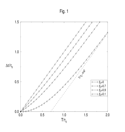
FIG. 1.: The function ${{\Delta\tau(T/\tau_{0})}\over{\tau_{0}}}$ versus $T/\tau_{0}$. Four typical cases are shown ($\beta_{0}=0$, $\beta_{0}=0.7$, $\beta_{0}=0.9$, $\beta_{0}=1$). All possible curve lines between the graphs of $\beta_{0}=0$ and $\beta_{0}=1$. The dashed line indicates the asymptotic behavior of the case $\beta_{0}=1$.

IV Derivation of the map

In the previous section we have shown the approximate solution for a charged particle circling in a uniform magnetic field. However, as mentioned above, the kicking of the electric field from Eq. (2) is with respect to the observed time $t$, and it is therefore convenient to integrate the equations of motion (Eqs. (16) and (17)) with respect to $t$.

A A charged particle in a uniform magnetic field - integration with respect to the observed time $t$

The arguments that were used in order to obtain Eqs. (18), as well as the implementation of the chain rule on Eqs. (16) and (17) by the use of Eq. (11) lead to the following equations of motion

$${{dq}\over{dt}} = -{1\over{\tau_{0}}}\sinh q$$ (26)

$${{d\phi}\over{dt}} = {\Omega\over{\cosh q}}.$$ (27)

A simple integration of Eq. (26) yields,

$$\tanh{q\over 2}=e^{C_{1}}e^{-{t\over{\tau_{0}}}},$$ (28)

where $C_{1}<0$. Substitution of Eq. (28) in Eq. (27) gives,

$${{d\phi}\over{dt}}=\Omega\tanh({t\over{\tau_{0}}}-C_{1}),$$ (29)

and the solution is

$$\phi=\Omega\tau_{0}\ln\cosh({t\over{\tau}}-C_{1})+C_{2},$$ (30)

where $C_{1}=\cosh^{-1}({1\over{\beta_{0}}})$, and $C_{2}=\tan^{-1}(\dot{y}_{0}/\dot{x}_{0})+\Omega\tau_{0}\ln\beta_{0}$. Returning to the original $x$, $y$ coordinates (using Eqs. (11)), the equations of motion become,

$${{dx}\over{dt}} = c{{\cos(\Omega\tau_{0}\ln(\cosh(t/\tau_{0}-C_{1}))+C_{2})}\over{\cosh(t/\tau_{0}-C_{1})}}$$ (31)

$${{dy}\over{dt}} = c{{\sin(\Omega\tau_{0}\ln(\cosh(t/\tau_{0}-C_{1}))+C_{2})}\over{\cosh(t/\tau_{0}-C_{1})}}.$$ (32)

It is possible to write Eq. (32) in more convenient way, by using the relation

$$\cosh({t\over{\tau_{0}}}-C_{1})={1\over{\beta_{0}}}\cosh{t\over{\tau_{0}}}+{1\over{\beta_{0}}}\sqrt{1-\beta_{0}^{2}}\sinh{t\over{\tau_{0}}}.$$ (33)

Eqs. (32) then become

$${{dx}\over{dt}} = {{\left({{dx}\over{dt}}\right)_{0}\cos\alpha-\left({{dy}\over{dt}}\right)_{0}\sin\alpha}\over{\cosh{t\over{\tau_{0}}}+\sqrt{1-\beta_{0}^{2}}\sinh{t\over{\tau_{0}}}}}$$ (34)

$${{dy}\over{dt}} = {{\left({{dx}\over{dt}}\right)_{0}\sin\alpha+\left({{dy}\over{dt}}\right)_{0}\cos\alpha}\over{\cosh{t\over{\tau_{0}}}+\sqrt{1-\beta_{0}^{2}}\sinh{t\over{\tau_{0}}}}},$$ (35)

where

$$\alpha=\Omega\tau_{0}\ln(\cosh{t\over{\tau_{0}}}(1+\sqrt{1-\beta_{0}^{2}}\tanh{t\over{\tau_{0}}})).$$ (36)

It is necessary to integrate Eq. (35) since the value of $x$ is used in the electric field kicking in Eq. (2). There is no analytical solution to Eq. (35), and a numerical integration must, in general, be performed. However, since we restrict ourselves to $T/\tau_{0}\ll 1$, it is possible to expand ${{dx}\over{dt}}$ and ${{dy}\over{dt}}$ in a Taylor series and then to integrate. The expansion of Eq. (36) is

$$\alpha\approx\Omega\sqrt{1-\beta_{0}^{2}}t+{1\over 2}\beta_{0}^{2}{{t^{2}}\over{\tau_{0}}}+{1\over 3}\sqrt{1-\beta_{0}^{2}}{{t^{3}}\over{\tau_{0}^{2}}}({3\over 2}-\beta_{0}^{2})+{\cal O}({{{t^{4}}\over{\tau_{0}^{3}}}}).$$ (37)

The first order expansion (according to $t/\tau_{0}$) of Eqs. (35) is

$${{dx}\over{dt}}={1\over{1+{1\over\gamma}{t\over{\tau_{0}}}}} \left[\left({{dx}\over{dt}}\right)_{0}\cos({{\Omega}\over\gamma}t+{1\over 2}\Omega\beta_{0}^{2}{{t^{2}}\over{\tau_{0}}})\right.$$ (39)

$$\left.-\left({{dy}\over{dt}}\right)_{0}\sin({{\Omega}\over\gamma}t+{1\over 2}\Omega\beta_{0}^{2}{{t^{2}}\over{\tau_{0}}})\right]$$

$${{dy}\over{dt}}={1\over{1+{1\over\gamma}{t\over{\tau_{0}}}}} \left[\left({{dx}\over{dt}}\right)_{0}\sin({{\Omega}\over\gamma}t+{1\over 2}\Omega\beta_{0}^{2}{{t^{2}}\over{\tau_{0}}})\right.$$ (41)

$$\left.+\left({{dy}\over{dt}}\right)_{0}\cos({{\Omega}\over\gamma}t+{1\over 2}\Omega\beta_{0}^{2}{{t^{2}}\over{\tau_{0}}})\right],$$

where $\gamma=1/\sqrt{1-\beta_{0}^{2}}$. Since ${1\over\gamma}{t\over{\tau_{0}}}\ll 1$, one can use the approximation,

$${1\over{1+{1\over\gamma}{t\over{\tau_{0}}}}}\approx{{1-{1\over\gamma}{t\over{\tau_{0}}}}}.$$ (42)

Using Eq. (42), the actual velocities, $dx/dt$ and $dy/dt$, from Eq. (41) can be integrated and expressed by elementary Fresnel functions. However, the effect of radiation is due to the ${1\over\gamma}{t\over{\tau_{0}}}$ term (which multiplies the sine and cosine functions), and the ${1\over 2}\Omega\beta_{0}^{2}{{t^{2}}\over{\tau_{0}}}$ term is not essential since the major offset from the unstable fixed point is due to the ${{\Omega}\over\gamma}t$ term.

Under the above assumptions the resulting equations are,

$$\left({{dx}\over{dt}}\right)_{T} = \left(1-{T\over{\gamma\tau_{0}}}\right)\times$$ (44)

$$\left[\left({{dx}\over{dt}}\right)_{0}\cos({{\Omega}\over\gamma}T)-\left({{dy}\over{dt}}\right)_{0}\sin({{\Omega}\over\gamma}T)\right]$$

$$\left({{dy}\over{dt}}\right)_{T} = \left(1-{T\over{\gamma\tau_{0}}}\right)\times$$ (46)

$$\left[\left({{dx}\over{dt}}\right)_{0}\sin({{\Omega}\over\gamma}T)+\left({{dy}\over{dt}}\right)_{0}\cos({{\Omega}\over\gamma}T)\right].$$

One therefore obtains

$$x_{T}\approx{\gamma\over\Omega}\left[\left({{dy}\over{dt}}\right)_{T}-\left({{dy}\over{dt}}\right)_{0}\right]-{\gamma\over{\Omega^{2}\tau_{0}}}\left[\left({{dx}\over{dt}}\right)_{T}-\left({{dx}\over{dt}}\right)_{0}\right]+x_{0}.$$ (47)

The exponential decay from Eqs. (32) are replaced by linear decay.

B Integration over a $\delta$ electric kick

As pointed out in the previous section, the Lorentz-Dirac equation (Eq. (1)) is a singular equation. The electric field which is used in this paper was expanded to a sum of $\delta$ functions (Eq. (2)). In that case, Eq. (1) can not be integrated over the kick by regular treatment, and some approximation for the $\delta$ function should be considered instead. In the present paper we assumed that the radiation during the kick is negligible; the radiation during the kick will be studied elsewhere. In addition, since the integration is over an infinitesimal time interval, there is no need to consider the constant magnetic field during the kick.

Under the above assumptions, in the neighborhood of the kick, the Lorentz-Dirac equation, Eq. (1), can be written as,

$${d\over{dt}}\left({{dx}\over{d\tau}}\right) = {f(x){\sum_{n=-\infty}^{\infty}\delta(t-nT)}}$$ (48)

$${d\over{dt}}\left({{dy}\over{d\tau}}\right) = 0.$$ (49)

Integration over the $\delta$ function yields,

$$\left({{dx}\over{d\tau}}\right)_{+} = \left({{dx}\over{d\tau}}\right)_{-}+f(x)$$ (50)

$$\left({{dy}\over{d\tau}}\right)_{+} = \left({{dy}\over{d\tau}}\right)_{-}$$ (51)

were the + sign indicates after the kick, and the - sign, before the kick. Following Ref. [1], we chose,

$$f(x)={{eET}\over{m_{0}}}\sin(kx)=K\sin(kx).$$ (52)

Using the fact that ${d\over{d\tau}}=\gamma{d\over{dt}}$ one obtains the following relations,

$$\gamma_{+} = \sqrt{1+{1\over{c^{2}}}\left[\left(\gamma_{-}\left({{dx}\over{dt}}\right)_{-}+f(x_{n})\right)^{2}+\gamma_{-}^{2}\left({{dy}\over{dt}}\right)_{-}^{2}\right]}$$ (55)

$$\left({{dx}\over{dt}}\right)_{+}={\gamma_{-}\over\gamma_{+}}\left({{dx}\over{dt}}\right)_{-}+{1\over\gamma_{+}}f(x_{n})$$

$$\left({{dy}\over{dt}}\right)_{+}={\gamma_{-}\over\gamma_{+}}\left({{dy}\over{dt}}\right)_{-}.$$

Returning to the initial charge $e=-e_{0}$ and thus $\Omega\to-\Omega$, the map which connects the velocities from just before the kick to the next kick (by the use of Eqs. (44)-(47)) is,

$$\left({{dx}\over{dt}}\right)_{n+1} =\left(1-{T\over{\gamma_{+}\tau_{0}}}\right)\times$$ (57)

$$\left[\left({{dx}\over{dt}}\right)_{+}\cos({{\Omega}\over{\gamma_{+}}}T)+\left({{dy}\over{dt}}\right)_{+}\sin({{\Omega}\over{\gamma_{+}}}T)\right]$$

$$\left({{dy}\over{dt}}\right)_{n+1} =\left(1-{T\over{\gamma_{+}\tau_{0}}}\right)\times$$ (59)

$$\left[-\left({{dx}\over{dt}}\right)_{+}\sin({{\Omega}\over{\gamma_{+}}}T)+\left({{dy}\over{dt}}\right)_{+}\cos({{\Omega}\over{\gamma_{+}}}T)\right]$$

$$x_{n+1} \approx-{{\gamma_{+}}\over\Omega}\left[\left({{dy}\over{dt}}\right)_{n+1}-\left({{dy}\over{dt}}\right)_{+}\right]$$ (61)

$$-{{\gamma_{+}}\over{\Omega^{2}\tau_{0}}}\left[\left({{dx}\over{dt}}\right)_{n+1}-\left({{dx}\over{dt}}\right)_{+}\right]+x_{n}.$$

Notice that the minus signs in Eq. (55) refer to the $n^{th}$ points of the map.

It is possible to return to the non-radiative limit by letting ${1\over{\tau_{0}}}\to 0$. In that case the map is equivalent to the map which was derived by Longcope and Sudan [3]. The nonrelativistic limit, which was derived by Zaslavskii et al [1], is achieved by letting ${1\over{\tau_{0}}}\to 0$ and $c\to\infty$.

C Analysis

Up to the derivation of Eqs. (57)-(61) we have passed three stages, (a) the velocities were calculated using an exact solution and the position $x$ can be calculated by numerical integration (Eqs. (35)), (b) the velocities were approximated by Eqs. (41) and the position $x$ by the elementary Fresnel function, and (c) the velocities were approximated by Eqs. (57)-(59) and the position $x$ (Eq. (61)) was derived using elementary integration. Among all the combinations of the solutions for the velocities and the position $x$ we choose the combination of the exact solution of velocities (case (a), Eqs. (35)) and the exact solution for the position $x$ (stage (c), Eq. (61)). The value of $x$ was selected from the third stage of our derivation since it enters the equation just in the kicking term, and there it affects only slightly the phase. Thus, one does not expect that this fact fact can change the typical behavior of the particle. The above analysis is summarized in Fig. 2.

FIG. 2.: A diagram which present the all possibilties for the map construction. The wider line indicates the chosen combination.

The radiative map is then

$$\left({{dx}\over{dt}}\right)_{n+1} = {{\left({{dx}\over{dt}}\right)_{+}\cos\alpha+\left({{dy}\over{dt}}\right)_{+}\sin\alpha}\over{\cosh{t\over{\tau_{0}}}+\sqrt{1-\beta_{+}^{2}}\sinh{t\over{\tau_{0}}}}}$$ (62)

$$\left({{dy}\over{dt}}\right)_{n+1} = {{-\left({{dx}\over{dt}}\right)_{+}\sin\alpha+\left({{dy}\over{dt}}\right)_{+}\cos\alpha}\over{\cosh{t\over{\tau_{0}}}+\sqrt{1-\beta_{+}^{2}}\sinh{t\over{\tau_{0}}}}}$$ (63)

$$x_{n+1} = -{{\gamma_{+}}\over\Omega}\left[\left({{dy}\over{dt}}\right)_{n+1}-\left({{dy}\over{dt}}\right)_{+}\right]$$ (65)

$$-{{\gamma_{+}}\over{\Omega^{2}\tau_{0}}}\left[\left({{dx}\over{dt}}\right)_{n+1}-\left({{dx}\over{dt}}\right)_{+}\right]+x_{n},$$

where the values immediately after the kick are as in Eqs. (55) and $\alpha$ is defined in Eq. (36) ($\alpha\to-\alpha$ since $e=-e_{0}$) . Note that for our limit ($T/\tau_{0}\ll 1$) there is not a great difference between the map given by Eqs. (57)-(61) and Eqs. (62)-(65).

V Results

In order to obtain a web structure, there are two conditions that have to fulfilled. In the nonrelativistic case, the first condition is that the ratio between the gyration frequency, $\Omega$, and the kicking time, $T$, is a rational number, a condition which can be expressed as follows,

$$\Omega T=2\pi{p\over q}$$ (66)

where $p$, and $q$, are integer numbers. Secondly, one must start from the neighborhood of the unstable fixed point (otherwise, the particle will not diffuse, and will not create a web structure),

$$\left({{dx}\over{dt}}\right)_{0} = 0$$ (67)

$$\left({{dy}\over{dt}}\right)_{0} \cong (2n+1){{\pi\Omega}\over k},$$ (68)

where $n$ is an integer number. The symmetry of the web is determined by $p$ and $q$. If, for example $p=1$ and $q=4$, the particle is kicked four times during one cycle, and thus, the symmetry of the web will be a four symmetry [1].

In the relativistic case [3], the above conditions are slightly different, because of the additional factor $\sqrt{1-\beta_{0}^{2}}$ which multiplies the $\Omega T$ term. However, if the initial velocities are small, i.e. $v_{0}\ll c$, the additional factor is close to 1, and thus the structure of the web should not change. In the radiative and relativistic case, as well as the non-radiative relativistic case, conditions (66) and (68) become,

$$\left({{dx}\over{dt}}\right)_{0} = 0$$ (69)

$$\left({{dy}\over{dt}}\right)_{0} \cong (2n+1)\sqrt{1-\beta_{0}^{2}}{{\pi\Omega}\over k}.$$ (70)

For sufficiently large initial velocities the above conditions do not hold anymore, and the web structure is not observed.

In this section we will compare (qualitatively; a quantitative treatment for the diffusions rate will be studied elsewhere) the diffusion of the non-radiative particle and the radiative particle. Intuitively, one would expect that a radiative particle will diffuse more slowly than a non-radiative one, since the radiation effects act like friction, and are thus expected to “stop” the particle. However, this naive explanation is not true, as we will demonstrate below.

In order to investigate the above assumption, we have chosen a four symmetry structure ($q=4$). We used the same initial conditions for all cases; just the kicking strength $K$ has been changed. The initial conditions were $B=10$, $v_{x,0}=0$, $v_{y,0}=4\times 10^{-5}$, $k=10$, and the number of iterations was $N=10^{6}$. In Fig. 3, we present the results as follows: the first column is the non-radiative case, the second column is the radiative case, and the third column is the total velocity versus the iteration number (the circles indicates the non-radiative case and the squares the radiative one). In the first row $K=1\times 10^{-5}$, in the second $K=2\times 10^{-5}$, and in the third $K=4\times 10^{-5}$.

As can be seen clearly from Fig. 3, the web structure is valid for the radiative case (top panel, first column). The web structure is also exists in the other cases; the web cells are very small and they are difficult to see. Although the radiative particle and the non-radiative particle start from the same initial conditions they behave differently.

In some cases the diffusion rate of the radiative case is larger then the diffusion rate of the non-radiative case, for example, in the top and the bottom panels after $9\times 10^{5}$ iterations the radiative particle reaches a higher velocity then the non-radiative one. On the other hand, in the middle panel the radiative particle is slower then non-radiative one. Obviously, it is impossible to draw any general conclusion for the question of whether a non-radiative particle is faster then the radiative one. For this a more systematic approach should be carried out. This would be beyond the scope of the present paper and will be considered elsewhere.

When the velocity of the particle reaches close to the velocity of light it actually stops growing (according to evolution in the time $t$) although it increases its energy. In Fig. 4 we show an example for that behavior. The parameters values are : $B=10$, $v_{x,0}=0$, $v_{y,0}=1\times 10^{-5}$, $k=10$, $K=0.01$, and the number of iterations was $N=1\times 10^{6}$ iterations (every $10^{\rm th}$ iteration was plotted). Fig. 4a and Fig. 4c are the non-radiative cases, while Fig. 4b and Fig. 4d are the radiative cases; in Fig. 4a and Fig. 4b the map of $v_{x}$ versus $v_{y}$ is presented, while in Fig. 4c and Fig. 4d the total velocity $v$ versus the iteration number is plotted (every $10^{\it th}$ iteration was plotted). As seen from Fig. 4, the particle accelerates quickly to high velocity, and most of the time stays with this high velocity, approaching light velocity asymptotically, while increasing its energy to infinity.

VI Summary and discussion

In the present paper we have investigated the effect of radiation on the stochastic web. Under the restriction of small magnetic fields ($B\lesssim{\cal O}(100T)$) an iterative map was constructed. Moreover, the effect of radiation on the stochastic web is very small because of the small magnetic field. Qualitatively, the non-radiative and the radiative cases have similar web structure. Despite of the naive expectation that the diffusion rate in the radiative case should be smaller then non-radiative case, one can find cases in which the opposite effect is observed.

Although it seems the effect of radiation is not qualitatively significant under laboratory conditions, it might have a strong effect in the presence of a strong magnetic field. Such a magnetic field could occur near or in a neuron star (or other heavy stars) and it can cause a large radiation correction to the motion of the particle. In that case one does not expect to have a web structure even when the particle has very small velocity, since the particle might move from the unstable fixed point and thus destroy the web structure. On the other hand, another scenario can take place; the magnetic field may be so strong that the particle almost stops its motion before the next kick, and under some symmetry conditions it can diffuse to the large energy regime. The described scheme can reflect new phenomenon not previously predicted, and could give some insight to the stellar systems.

In the present study we did not consider the radiation during the $\delta$ kick because of lack of proper technical methods as well as analytical knowledge. Taking into account the radiation during the kick could change our conclusions, and as for other open questions which mentioned in this paper, this point will be treated elsewhere.

We would like to thank I. Dana for helpful discussions.

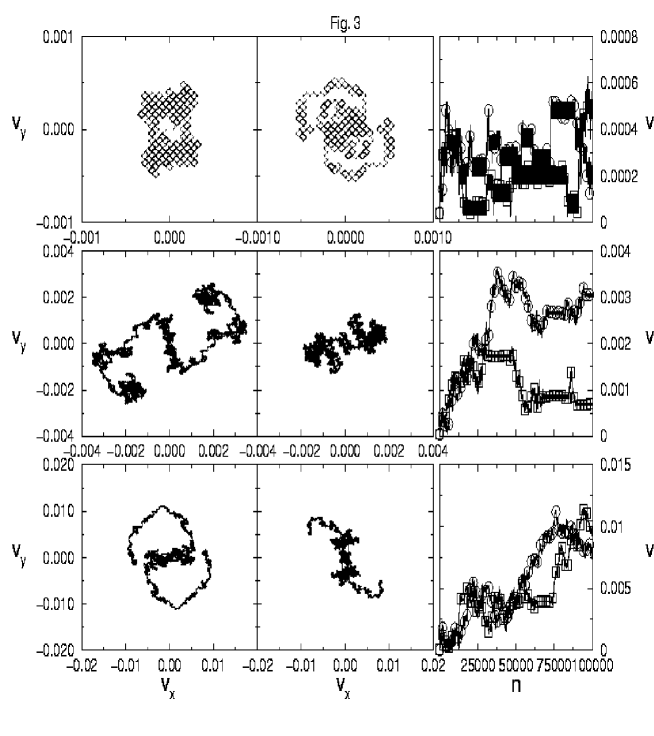
FIG. 3.: Different types of diffusion behavior as described in the context.

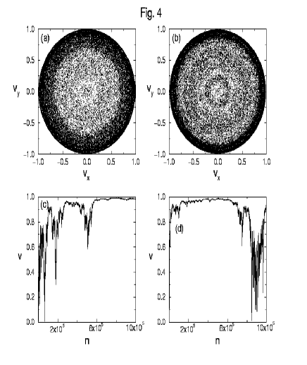
FIG. 4.: The behavior of a particle with high velocity. (a) the nonradiative map map, (b) the radiative map, (c) the total velocity of the non-radiative case, and (d) the total velocity of the radiative case.

REFERENCES

- [1] G.M. Zaslavskii, M.Yu. Zakharov, R.Z. Sagdeev, D.A. Usikov, and A.A. Chernikov, Zh. Eksp. Teor. Fiz 91, 500 (1986) [Sov. Phys. JEPT 64, 294 (1986)].
- [2] V.I. Arnold’d, Dokl. Akad. Nauk. SSSR 159, 9 (1964).
- [3] D.W. Longcope and R.N. Sudan, Phys. Rev. Lett. 59, 1500 (1987); See also, A.J. Lichtenberg and M.A. Lieberman, Regular and Chaotic Dynamics 2nd ed., (Springer-Verlag, New York, 1992).
- [4] H. Karimabadi and V. Angelopoulos, Phys. Rev. Lett. 62, 2342 (1989).
- [5] We thank T. Goldman for comments on the mechanism for this bound in our equation during a seminar at Los Alamos.
- [6] L.P. Horwitz and Y. Ashkenazy, Discrete Dynamics in Nature and Society, this issue.
- [7] M. Abraham, Theorie der Elektrizität, vol. II, Springer, Leipzig (1905). See ref. [9] for a discussion of the origin of these terms; P.A.M. Dirac, Proc. Roy. Soc. London Ser. A, 167, 148 (1938).
- [8] A.A. Sokolov and I.M. Ternov, Radiation from Relativistic Electrons, Amer. Inst. of Phys. Translation Series, New York (1986).
- [9] F. Rohrlich, Classical Charged Particles, Addison Wesley, Reading, Mass. (1965).
- [10] J.M. Aguirrebiria, J. Phys. A Math. Gen. 30, 2391 (1997).