Bicritical Behavior of Period Doublings in Unidirectionally-Coupled Maps

Abstract

We study the scaling behavior of period doublings in two unidirectionally-coupled one-dimensional maps near a bicritical point where two critical lines of period-doubling transition to chaos in both subsystems meet. Note that the bicritical point corresponds to a border of chaos in both subsystems. For this bicritical case, the second response subsystem exhibits a new type of non-Feigenbaum critical behavior, while the first drive subsystem is in the Feigenbaum critical state. Using two different methods, we make the renormalization group analysis of the bicritical behavior and find the corresponding fixed point of the renormalization transformation with two relevant eigenvalues. The scaling factors obtained by the renormalization group analysis agree well with those obtained by a direct numerical method.

I Introduction

Period-doubling transition to chaos has been extensively studied in a one-parameter family of one-dimensional (1D) unimodal maps,

$$x_{t+1}=1-Ax_{t}^{2},$$ (1)

where $x_{t}$ is a state variable at a discrete time $t$. As the control parameter $A$ is increased, the 1D map undergoes an infinite sequence of period-doubling bifurcations accumulating at a critical point $A_{c}$, beyond which chaos sets in. Using a renormalization group (RG) method, Feigenbaum [1] has discovered universal scaling behavior near the critical point $A_{c}$.

Here we are interested in the period doublings in a system consisting of two 1D maps with a one-way coupling,

$$x_{t+1}=1-Ax_{t}^{2},\;\;y_{t+1}=1-By_{t}^{2}-Cx_{t}^{2},$$ (2)

where $x$ and $y$ are state variables of the first and second subsystems, $A$ and $B$ are control parameters of the subsystems, and $C$ is a coupling parameter. Note that the first (drive) subsystem acts on the second (response) subsystem, while the second subsystem does not influence the first subsystem. This kind of unidirectionally-coupled 1D maps are used as a model for open flow [2]. A new kind of non-Feigenbaum scaling behavior was found in a numerical and empirical way near a bicritical point $(A_{c},B_{c})$ where two critical lines of period-doubling transition to chaos in both subsystems meet [3]. For this bicritical case, a RG analysis was also developed and the corresponding fixed point, governing the bicritical behavior, was numerically obtained by directly solving the RG fixed-point equation using a polynomial approximation [4]. In this paper, using two different methods, we also make the RG analysis of the bicriticality, the results of which agree well with those of previous works.

This paper is organized as follows. In Sec. II we study the scaling behavior near a bicritical point $(A_{c},B_{c})$, corresponding to a border of chaos in both subsystems, by directly following a period-doubling sequence converging to the point $(A_{c},B_{c})$ for a fixed value of $C$. For this bicritical case, a new type of non-Feigenbaum critical behavior appears in the second subsystem, while the first subsystem is in the Feigenbaum critical state. Employing two different methods, we make the RG analysis of the bicritical behavior in Sec. III. To solve the RG fixed-point equation, we first use an approximate truncation method [5], corresponding to the lowest-order polynomial approximation. Thus we analytically obtain the fixed point, associated with the bicritical behavior, and its relevant eigenvalues. Compared with the previous numerical results [4], these analytic results are not bad as the lowest-order approximation. To improve accuracy, we also employ the “eigenvalue-matching” RG method [6], equating the stability multipliers of the orbit of level $n$ (period $2^{n}$) to those of the orbit of the next level $n+1$. Thus we numerically obtain the bicritical point, the parameter and orbital scaling factors, and the critical stability multipliers. We note that the accuracy is improved remarkably with increasing the level $n$. Finally, a summary is given in Sec. IV.

II Scaling Behavior near The Bicritical Point

In this section we fix the value of the coupling parameter by setting $C=0.45$ and directly follow a period-doubling sequence converging to the bicritical point $(A_{c},B_{c})$, which corresponds to a border of chaos in both subsystems. For this bicritical case, the second subsystem exhibits a new type of non-Feigenbaum critical behavior, while the first subsystem is in the Feigenbaum critical state.

The unidirectionally-coupled 1D maps (2) has many attractors for fixed values of the parameters [7]. For the case $C=0$, it breaks up into the two uncoupled 1D maps. If they both have stable orbits of period $2^{k}$, then the composite system has $2^{k}$ different stable states distinguished by the phase shift between the subsystems. This multistability is preserved when the coupling is introduced, at least while its value is small enough. Here we study only the attractors whose basins include the origin $(0,0)$. Such attractors become in-phase when $A=B$ and $C=0$.

Stability of an orbit with period $q$ is determined by its stability multipliers,

$$\lambda_{1}=\prod_{t=1}^{q}-2Ax_{t},\;\;\lambda_{2}=\prod_{t=1}^{q}-2By_{t}.$$ (3)

Here $\lambda_{1}$ and $\lambda_{2}$ determine the stability of the first and second subsystems, respectively. An orbit becomes stable when the moduli of both multipliers are less than unity, i.e., $-1<\lambda_{i}<1$ for $i=1,2$.

FIG. 1.: Stability diagram of the periodic orbits born via period-doubling bifurcations for $C=0.45$. The numbers in the different regions represent the period of motion in the second subsystem. The open circle also denotes the point, corresponding to a threshold of instability in both subsystems, where $\lambda_{1}=-1$ and $\lambda_{2}=-1$. Such open circles accumulate to the bicritical point, denoted by the solid circle, which corresponds to a border of chaos in both subsystems. For other details, see the text.

Figure 1 shows the stability diagram of periodic orbits for $C=0.45$. As the parameter $A$ is increased, the first subsystem exhibits a sequence of period-doubling bifurcations at the vertical straight lines, where $\lambda_{1}=-1$. For small values of the parameter $B$, the period of oscillation in the second subsystem is the same as that in the first subsystem, as in the case of forced oscillation. As $B$ is increased for a fixed value of $A$, a sequence of period-doubling bifurcations occurs in the second subsystem when crossing the non-vertical lines where $\lambda_{2}=-1$. The numbers inside the different regions denote the period of the oscillation in the second subsystem.

We consider a pair of the parameters $(A_{n},B_{n})$, at which the periodic orbit of level $n$ (period $2^{n}$) has the stability multipliers $\lambda_{1,n}=\lambda_{2,n}=-1$. Hence, the point $(A_{n},B_{n})$ corresponds to a threshold of instability in both subsystems. Some of such points are denoted by the open circles in Fig. 1. Then such a sequence of $(A_{n},B_{n})$ converges to the bicritical point $(A_{c},B_{c})$, corresponding to a border of chaos in both systems, with increasing the level $n$. The bicritical point is denoted by the solid circle in Fig. 1. To locate the bicritical point with a satisfactory precision, we numerically follow the orbits of period $q=2^{n}$ up to level $n=21$ in a quadruple precision, and obtain the sequences of both the parameters $(A_{n},B_{n})$ and the orbit points $(x_{n},y_{n})$ approaching the origin. We first note that the sequences of $A_{n}$ and $x_{n}$ in the first subsystem are the same as those in the 1D maps [1]. Hence, only the sequences of $B_{n}$ and $y_{n}$ in the second subsystem are given in Table I.

TABLE I.: Sequences of the parameter and the orbit point, $\{B_{n}\}$ and $\{y_{n}\}$, in the second subsystem.

$n$	$B_{n}$	$y_{n}$
10	1.090 088 955 364	5.019 189 $\times$$10^{-3}$
11	1.090 092 109 910	-3.333 775 $\times$$10^{-3}$
12	1.090 093 416 851	2.214 467 $\times$$10^{-3}$
13	1.090 093 959 979	-1.471 024 $\times$$10^{-3}$
14	1.090 094 186 392	9.771 970 $\times$$10^{-4}$
15	1.090 094 280 906	-6.491 561 $\times$$10^{-4}$
16	1.090 094 320 376	4.312 391 $\times$$10^{-4}$
17	1.090 094 336 865	-2.864 762 $\times$$10^{-4}$
18	1.090 094 343 755	1.903 092 $\times$$10^{-4}$
19	1.090 094 346 634	-1.264 245 $\times$$10^{-4}$
20	1.090 094 347 837	8.398 518 $\times$$10^{-5}$
21	1.090 094 348 340	-5.579 230 $\times$$10^{-5}$

We now study the asymptotic scaling behavior of the period-doubling sequences in both subsystems near the bicritical point. The scaling behavior in the first subsystem is obviously the same as that in the 1D maps [1]. That is, the sequences $\{A_{n}\}$ and $\{x_{n}\}$ accumulate to their limit values, $A=A_{c}$ $(=1.401\,155\,189\,092\cdots)$ and $x=0$, geometrically as follows:

$$A_{n}-A_{c}\sim\delta_{1}^{-n},\;\;x_{n}\sim\alpha_{1}^{-n}\;\;{\rm for\;large\;}n.$$ (4)

The scaling factors $\delta_{1}$ and $\alpha_{1}$ are just the Feigenbaum constants $\delta$ $(=4.669\cdots)$ and $\alpha$ $(=-2.502\cdots)$ for the 1D maps, respectively. However, the second subsystem exhibits a non-Feigenbaum critical behavior, unlike the case of the first subsystem. The two sequences $\{B_{n}\}$ and $\{y_{n}\}$ also converge geometrically to their limit values $B=B_{c}$ $(=1.090\,094\,348\,701)$ and $y=0$, respectively, where the value of $B_{c}$ is obtained using the superconverging method [8]. To obtain the convergence rates of the two sequences, we define the scaling factors of level $n$:

$$\delta_{2,n}\equiv{{B_{n-1}-B_{n}}\over{B_{n}-B_{n+1}}},\;\;\alpha_{2,n}\equiv{{y_{n-1}-y_{n}}\over{y_{n}-y_{n+1}}}.$$ (5)

These two sequences $\{\delta_{2,n}\}$ and $\{\alpha_{2,n}\}$ are listed in Table II, and they converge to their limit values,

$$\delta_{2}\simeq 2.3928,\;\;\alpha_{2}\simeq-1.5053,$$ (6)

respectively. Note that these scaling factors are completely different from those in the first subsystem (i.e., the Feigenbaum constants for the 1D maps).

TABLE II.: Sequences of the parameter and orbital scaling factors, $\{\delta_{2,n}\}$ and $\{\alpha_{2,n}\}$, in the second subsystem.

$n$	$\delta_{2,n}$	$\alpha_{2,n}$
10	2.429 8	-1.505 733 1
11	2.413 7	-1.505 515 4
12	2.406 3	-1.505 428 1
13	2.398 8	-1.505 375 3
14	2.395 6	-1.505 344 0
15	2.394 6	-1.505 331 6
16	2.393 7	-1.505 325 6
17	2.393 1	-1.505 321 5
18	2.393 0	-1.505 319 8
19	2.392 9	-1.505 319 1
20	2.392 8	-1.505 318 6

For evidence of scaling, we compare the chaotic attractors, shown in Fig. 2, for the three values of $(A,B)$ near the bicritical point $(A_{c},B_{c})$. All these attractors are the hyperchaotic ones with two positive Lyapunov exponents [9],

$$\sigma_{1} = \lim_{m\rightarrow\infty}{1\over m}\sum_{t=1}^{m}\ln|2Ax_{t}|,\;\;\sigma_{2}=\lim_{m\rightarrow\infty}{1\over m}\sum_{t=1}^{m}\ln|2By_{t}|.$$ (7)

Here the first and second Lyapunov exponents $\sigma_{1}$ and $\sigma_{2}$ denote the average exponential divergence rates of nearby orbits in the the first and second subsystems, respectively. Figure 2(a) shows the hyperchaotic attractor with $\sigma_{1}\simeq 0.242$ and $\sigma_{2}\simeq 0.04$ for $A=A_{c}+\Delta A$ and $B=B_{c}+\Delta B$, where $\Delta A=\Delta B=0.1$. This attractor consists of two pieces. To see scaling, we first rescale $\Delta A$ and $\Delta B$ with the parameter scaling factors $\delta_{1}$ and $\delta_{2}$, respectively. The attractor for the rescaled parameter values of $A=A_{c}+\Delta A/\delta_{1}$ and $B=B_{c}+\Delta B/\delta_{2}$ is shown in Fig. 2(b). It is also the hyperchaotic attractor with $\sigma_{1}\simeq 0.121$ and $\sigma_{2}\simeq 0.02$. We next magnify the region in the small box (containing the origin) by the scaling factor $\alpha_{1}$ for the $x$ axis and $\alpha_{2}$ for the $y$ axis, and then we get the picture in Fig. 2(c). Note that the picture in Fig. 2(c) reproduces the previous one in Fig. 2(a) approximately. Repeating the above procedure once more, we obtain the two pictures in Figs. 2(d) and 2(e). That is, Fig. 2(d) shows the hyperchaotic attractor with $\sigma\simeq 0.061$ and $\sigma_{2}\simeq 0.01$ for $A=A_{c}+\Delta A/\delta_{1}^{2}$ and $B=B_{c}+\Delta B/\delta_{2}^{2}$. Magnifying the region in the small box with the scaling factors $\alpha_{1}^{2}$ for the $x$-axis and $\alpha_{2}^{2}$ for the $y$-axis, we also obtain the picture in Fig. 2(e), which reproduces the previous one in Fig. 2(c) with an increased accuracy.

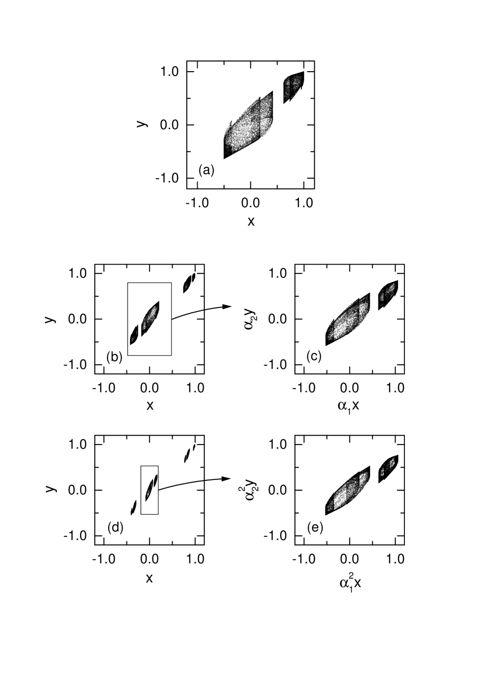
FIG. 2.: Hyperchaotic attractors for the three values of $(A,B)$ near the bicritical point $(A_{c}.B_{c})$; in (a) $(A,B)=(A_{c}+\Delta A,B_{c}+\Delta B)$ $(\Delta A=\Delta B=0.1)$, in (b) and (c) $(A,B)=(A_{c}+\Delta A/\delta_{1},B_{c}+\Delta B/\delta_{2})$, and in (d) and (e) $(A,B)=(A_{c}+\Delta A/\delta_{1}^{2},B_{c}+\Delta B/\delta_{2}^{2})$. The picture in (c) is obtained by magnifying the region in the small box in (b) with the scaling factors $\alpha_{1}$ for the $x$-axis and $\alpha_{2}$ for the $y$-axis. Similarly, we also obtain the picutre (e) by magnifying the region inside the small box in (d) with the scaling factors $\alpha_{1}^{2}$ for the $x$-axis and $\alpha_{2}^{2}$ for the $y$-axis. Comparing the pictures in (a), (c), and (e), one can see that each successive magnified picture reproduces the previous one with an accuracy with the depth of resolution.

So far we have seen the scaling near the bicritical point, and now turn to a discussion of the behavior exactly at the bicritical point $(A_{c},B_{c})$. There exist an infinity of unstable periodic orbits with period $2^{n}$ at the bicritical point. The orbit points $x_{n}$ and $y_{n}$, approaching the zero in the first and second subsystems, vary asymptotically in proportion to $\alpha_{1}^{-n}$ and $\alpha_{2}^{-n}$, respectively. The stability multipliers $\lambda_{1,n}$ and $\lambda_{2,n}$ of the orbits with period $2^{n}$ also converge to the critical stability multipliers $\lambda_{1}^{*}$ and $\lambda_{2}^{*}$, respectively. Here $\lambda_{1}^{*}$ $(=-1.601\,191\,\cdots)$ in the first subsystem is just the critical stability multiplier for the case of the 1D maps [1]. However, as listed in Table III, the second subsystem has the different critical stability multiplier,

$$\lambda_{2}^{*}=-1.178\,85\,\cdots.$$ (9)

Consequently, the periodic orbits at the bicritical point have the same stability multipliers $\lambda_{1}^{*}$ and $\lambda_{2}^{*}$ for sufficiently large $n$.

TABLE III.: Sequences of the second stability multipliers, $\{\lambda_{2,n}\}$ of the orbits with period $2^{n}$ at the bicritical point.

$n$	$\lambda_{2,n}$
10	-1.178 829
11	-1.178 842
12	-1.178 839
13	-1.178 850
14	-1.178 855
15	-1.178 854
16	-1.178 854
17	-1.178 855
18	-1.178 855
19	-1.178 854

III Renormalization Group Analysis of The Bicritical Behavior

Employing two different methods, we make the RG analysis of the bicritical behavior. We first use the truncation method, and analytically obtain the corresponding fixed point and its relevant eigenvalues. These analytic results are not bad as the lowest-order approximation. To improve the accuracy, we also use the numerical eigenvalue-matching method, and obtain the bicritical point, the parameter and orbital scaling factors, and the critical stability multipliers. Note that the accuracy in the numerical RG results is improved remarkably with increasing the level $n$.

A Truncation Method

In this subsection, employing the truncation method [5], we analytically make the RG analysis of the bicritical behavior in the unidirectionally-coupled map T of the form,

$$T:\;x_{t+1}=f(x_{t}),\;\;y_{t+1}=g(x_{t},y_{t}),$$ (10)

where $x_{t}$ and $y_{t}$ are the state variables at a discrete time $t$ in the first and second subsystems, respectively. Truncating the map (10) at its quadratic terms, we have

$$T_{{\bf P}}:\;x_{t+1}={a\over b}+bx_{t}^{2},\;\;y_{t+1}={c\over d}+dy_{t}^{2}+{e\over d}x_{t}^{2},$$ (11)

which is a five-parameter family of unidirecionally-coupled maps. $\bf P$ represents the five parameters, i.e., ${\bf P}=(a,b,c,d,e)$. The construction of Eq. (11) corresponds to a truncation of the infinite dimensional space of unidirectionally-coupled maps to a five-dimensional space. The parameters $a,b,c,d,$ and $e$ can be regarded as the coordinates of the truncated space. We also note that this truncation method corresponds to the lowest-order polynomial approximation.

We look for fixed points of the renormalization operator ${\cal R}$ in the truncated five-dimensional space of unidirectionally-coupled maps,

$${\cal R}(T)=\Lambda T^{2}\Lambda^{-1}.$$ (12)

Here the rescaling operator $\Lambda$ is given by

$$\Lambda=\left(\begin{array}[]{cc}\alpha_{1}&0\\ 0&\alpha_{2}\end{array}\right),$$ (13)

where $\alpha_{1}$ and $\alpha_{2}$ are the rescaling factors in the first and second subsystems, respectively.

The operation ${\cal R}$ in the truncated space can be represented by a transformation of parameters, i.e., a map from ${\bf P}\equiv(a,b,c,d,e)$ to ${\bf P^{\prime}}\equiv(a^{\prime},b^{\prime},c^{\prime},d^{\prime},e^{\prime}),$

$$a^{\prime} = 2a^{2}(1+a),$$ (15)

$$b^{\prime} = {2\over\alpha_{1}}ab,$$ (16)

$$c^{\prime} = 2c(c+c^{2}+e{a^{2}\over b^{2}}),$$ (17)

$$d^{\prime} = {2\over\alpha_{2}}cd,$$ (18)

$$e^{\prime} = {4\over\alpha_{1}^{2}}ce(a+c).$$ (19)

The fixed point ${\bf P}^{*}=(a^{*},b^{*},c^{*},d^{*},e^{*})$ of this map can be determined by solving ${\bf P}^{\prime}={\bf P}$. The parameters $b$ and $d$ set only the scales in the $x$ and $y$, respectively, and thus they are arbitrary. We now fix the scales in $x$ and $y$ by setting $b=d=1$. Then, we have, from Eqs.(15)-(19), five equations for the five unknowns $\alpha_{1},a^{*},\alpha_{2},c^{*},$ and $e^{*}$. We thus find one solution, associated with the bicritical behavior, as will be seen below. The map (11) with a solution ${\bf P^{*}}$ $(T_{{\bf P^{*}}})$ is the fixed map of the renormalization transformation ${\cal R}$; for brevity $T_{{\bf P^{*}}}$ will be denoted as $T^{*}$.

We first note that Eqs. (15)-(16) are only for the unknowns $\alpha_{1}$ and $a^{*}$. We find one solution for $\alpha_{1}$ and $a^{*}$, associated with the period-doubling bifurcation in the first subsystem,

$$\alpha_{1}=-1-\sqrt{3}=-2.732\cdots,\;a^{*}={\alpha_{1}\over 2}.$$ (20)

Substituting the values for $\alpha_{1}$ and $a^{*}$ into Eqs. (17)-(19), we obtain one solution for $\alpha_{2}$, $c^{*}$, and $e^{*}$, associated with the bicriticality,

$$\alpha_{2} = {1\over 2}(1+\sqrt{3}-\sqrt{5}-\sqrt{15})=-1.688\cdots,$$ (22)

$$c^{*} = {\alpha_{2}\over 2},\;\;e^{*}=1+{1\over 2}(\sqrt{15}-3\sqrt{3})=0.338\cdots.$$ (23)

Compared with the values, $\alpha_{1}=-2.502\cdots$ and $\alpha_{2}=-1.505\cdots$, obtained by a direct numerical method, the analyitc results for $\alpha_{1}$ and $\alpha_{2}$, given in Eqs. (20) and (22), are not bad as the lowest-order approximation.

Consider an infinitesimal perturbation $\epsilon\,\delta{\bf P}$ to a fixed point ${\bf P}^{*}$ of the transformation of parameters (15)-(19). Linearizing the transformation at ${\bf P}^{*}$, we obtain the equation for the evolution of $\delta{\bf P}$,

$$\delta{\bf P}^{\prime}=J\delta{\bf P},$$ (24)

where $J$ is the Jacobian matrix of the transformation at ${\bf P}^{*}$.

The $5\times 5$ Jacobian matrix $J$ has a semi-block form, because we are considering the unidirectionally-coupled case. Therefore, one can easily obtain its eigenvalues. The first two eigenvalues, associated with the first subsystem, are those of the following $2\times 2$ matrix,

$$\left.M_{1}={\frac{{\partial(a^{\prime},b^{\prime})}}{{\partial(a,b)}}}\right|_{{\bf P^{*}}}=\left(\begin{array}[]{cc}3-\alpha_{1}&0\\ {2/\alpha_{1}}&1\end{array}\right).$$ (27)

Hence the two eigenvalues of $M_{1}$, $\delta_{1}$ and $\delta_{1}^{\prime}$, are given by

$$\delta_{1}=4+\sqrt{3}=5.732\cdots,\;\;\delta_{1}^{\prime}=1.$$ (28)

Here the relevant eigenvalue $\delta_{1}$ is associated with the scaling of the control parameter in the first subsystem, while the marginal eigenvalue $\delta_{1}^{\prime}$ is associated with the scale change in $x$. When compared with the numerical value, $\delta_{1}$ $(=4.669\cdots)$, the analytic result for $\delta_{1}$, given in Eq. (28), is not bad as the lowest-order approximation.

The remaining three eigenvalues, associated with the second subsystem, are those of the following $3\times 3$ matrix,

$$\left.M_{2}={\frac{{\partial(c^{\prime},d^{\prime},e^{\prime})}}{{\partial(c,d,e)}}}\right|_{{\bf P^{*}}}=\left(\begin{array}[]{ccc}4c^{*}+6c^{*2}+2a^{*2}e^{*}&0&2a^{*2}c^{*}\\ 2/\alpha_{2}&2c^{*}/\alpha_{2}&0\\ 4e^{*}(a^{*}+2c^{*})/\alpha_{1}^{2}&0&4c^{*}(a^{*}+c^{*})/\alpha_{1}^{2}\end{array}\right).$$ (29)

The three eigenvalues of $M_{2}$, $\delta_{2}$, $\delta_{2}^{\prime}$, and $\delta_{2}^{\prime\prime}$, are given by

$$\delta_{2} = (u+\sqrt{v})/2=3.0246\cdots,$$ (31)

$$\delta_{2}^{\prime} = (u-\sqrt{v})/2=0.1379\cdots,\;\;\delta_{2}^{\prime\prime}=1,$$ (32)

where

$$u = (17+7\sqrt{3}-5\sqrt{5}-3\sqrt{15})/2,$$ (34)

$$v = 104+53\sqrt{3}-44\sqrt{5}-23\sqrt{15}.$$ (35)

The first eigenvalue $\delta_{2}$ is a relevant eigenvalue, associated with the scaling of the control parameter in the second subsystem, the second eigenvalue $\delta_{2}^{\prime}$ is an irrelavant one, and the third eigenvalue $\delta_{2}^{\prime\prime}$ is a marginal eigenvalue, associated with the scale change in $y$. We also compare the analytic result for $\delta_{2}$, given in Eq. (31), with the numerical value $(\delta_{2}\simeq 2.3928)$ in Eq. (6), and find that the analytic one is not bad as the lowest-order approximation.

As shown in Sec. II, stability multipliers of an orbit with period $2^{n}$ at the bicritical point converge to the critical stability multipliers, $\lambda_{1}^{*}$ $(=-1.601\cdots)$ and $\lambda_{2}^{*}$ $(=-1.178\cdots)$ as $n\rightarrow\infty$. We now obtain these critical stability analytically. The invariance of the fixed map $T^{*}$ under the renormalization transformation $\cal R$ implies that, if $T^{*}$ has a periodic point $(x,y)$ with period $2^{n}$, then $\Lambda^{-1}(x,y)$ is a periodic point of $T^{*}$ with period $2^{n+1}$. Since rescaling does not affect the stability multipliers, all the orbits with period $2^{n}$ $(n=0,1,2,\dots)$ have the same stability multipliers, which are just the critical stability multipliers $\lambda_{1}^{*}$ and $\lambda_{2}^{*}$. That is, the critical stability multipliers have the values of the stability multipliers of the fixed point $(x^{*},y^{*})$ of the fixed map $T^{*}$,

$$\lambda_{1}^{*}=2x^{*}=-1.5424\cdots,\;\;\lambda_{2}^{*}=2y^{*}=-0.8899\cdots,$$ (36)

where

$$x^{*} = (1-\sqrt{3+2\sqrt{3}})/2,\;\;y^{*}=(1-\sqrt{w})/2,$$ (38)

$$w = 5+3\sqrt{3}-2\sqrt{5}-\sqrt{15}$$ (40)

$$+\sqrt{3+2\sqrt{3}}\;(2-3\sqrt{3}+\sqrt{15}).$$

We also note that the analytic values for $\lambda^{*}_{1}$ and $\lambda^{*}_{2}$ are not bad, when compared with their numerical values.

B Eigenvalue-Matching Method

In this subsection, we employ the eigenvalue-matching method [6] and numerically make the RG analysis of the bicritical behavior in the unidirectionally-coupled map $T$ of Eq. (2). As the level $n$ increases, the accuracy in the numerical RG results are remarkably improved.

The basic idea is to associate a value $(A^{\prime},B^{\prime})$ for each value $(A,B)$ such that $T^{(n+1)}_{(A^{\prime},B^{\prime})}$ locally resembles $T^{(n)}_{(A,B)}$, where $T^{(n)}$ is the $2^{n}$th-iterated map of $T$ (i.e., $T^{(n)}=T^{2^{n}}$). A simple way to implement this idea is to linearize the maps in the neighborhood of their respective fixed points and equate the corresponding eigenvalues.

Let $\{z_{t}\}$ and $\{z^{\prime}_{t}\}$ be two successive cycles of period $2^{n}$ and $2^{n+1}$, respectively, i.e.,

$$z_{t}=T^{(n)}_{(A,B)}(z_{t}),\;\;z^{\prime}_{t}=T^{(n+1)}_{(A^{\prime},B^{\prime})}(z^{\prime}_{t});\;z_{t}=(x_{t},y_{t}).$$ (41)

Here $x_{t}$ depends only on $A$, but $y_{t}$ is dependent on both $A$ and $B$, i.e., $x_{t}=x_{t}(A)$ and $y_{t}=y_{t}(A,B)$. Then their linearized maps at $z_{t}$ and $z^{\prime}_{t}$ are given by

$$DT^{(n)}_{(A,B)} = \prod_{t=1}^{2^{n}}DT_{(A,B)}(z_{t}),$$ (43)

$$DT^{(n+1)}_{(A^{\prime},B^{\prime})} = \prod_{t=1}^{2^{n+1}}DT_{(A^{\prime},B^{\prime})}(z^{\prime}_{t}).$$ (44)

(Here $DT$ is the linearized map of $T$.) Let their eigenvalues, called the stability multipliers, be ($\lambda_{1,n}(A),\lambda_{2,n}(A,B))$ and ($\lambda_{1,n+1}(A^{\prime}),\lambda_{2,n+1}(A^{\prime},B^{\prime}))$. The recurrence relations for the old and new parameters are then given by equating the stability multipliers of level $n$, $\lambda_{1,n}(A)$ and $\lambda_{2,n}(A,B)$, to those of the next level $n+1$, $\lambda_{1,n+1}(A^{\prime})$ and $\lambda_{2,n+1}(A^{\prime},B^{\prime})$, i.e.,

$$\lambda_{1,n}(A) = \lambda_{1,n+1}(A^{\prime}),$$ (46)

$$\lambda_{2,n}(A,B) = \lambda_{2,n+1}(A^{\prime},B^{\prime}).$$ (47)

The fixed point $(A^{*},B^{*})$ of the renormalization transformation (III B),

$$\lambda_{1,n}(A^{*}) = \lambda_{1,n+1}(A^{*}),$$ (49)

$$\lambda_{2,n}(A^{*},B^{*}) = \lambda_{2,n+1}(A^{*},B^{*}).$$ (50)

gives the bicritical point $(A_{c},B_{c})$. By linearizing the renormalization transformation (III B) at the fixed point $(A^{*},B^{*})$, we have

$$\left(\begin{array}[]{c}\Delta A\\ \Delta B\end{array}\right) = \left(\begin{array}[]{cc}\left.{\partial A\over\partial A^{\prime}}\right|_{*}&\left.{\partial A\over\partial B^{\prime}}\right|_{*}\\ \left.{\partial B\over\partial A^{\prime}}\right|_{*}&\left.{\partial B\over\partial B^{\prime}}\right|_{*}\end{array}\right)\left(\begin{array}[]{c}\Delta A^{\prime}\\ \Delta B^{\prime}\end{array}\right)$$ (57)

$$= \Delta_{n}\left(\begin{array}[]{c}\Delta A^{\prime}\\ \Delta B^{\prime}\end{array}\right),$$ (60)

where $\Delta A=A-A^{*}$, $\Delta B=B-B^{*}$, $\Delta A^{\prime}=A^{\prime}-A^{*}$, $\Delta B^{\prime}=B^{\prime}-B^{*}$, and

$$\Delta_{n} = \Gamma_{n}^{-1}\Gamma_{n+1};$$ (62)

$$\Gamma_{n} = \left(\begin{array}[]{cc}\left.{{d\lambda_{1,n}\over dA}}\right|_{*}&0\\ \left.{{\partial\lambda_{2,n}\over\partial A}}\right|_{*}&\left.{{\partial\lambda_{2,n}\over\partial B}}\right|_{*}\end{array}\right),$$ (65)

$$\Gamma_{n+1} = \left(\begin{array}[]{cc}\left.{{d\lambda_{1,n+1}\over dA^{\prime}}}\right|_{*}&0\\ \left.{{\partial\lambda_{2,n+1}\over\partial A^{\prime}}}\right|_{*}&\left.{{\partial\lambda_{2,n+1}\over\partial B^{\prime}}}\right|_{*}\end{array}\right).$$ (68)

Here $\Gamma_{n}^{-1}$ is the inverse of $\Gamma_{n}$ and the asterisk denotes the fixed point $(A^{*},B^{*})$. After some algebra, we obtain the analytic formulas for the eigenvalues $\delta_{1,n}$ and $\delta_{2,n}$ of the matrix $\Delta_{n}$,

$$\delta_{1,n} = {{\left.{d\lambda_{1,n+1}\over dA^{\prime}}\right|_{*}}\over{\left.{d\lambda_{1,n}\over dA}\right|_{*}}},$$ (70)

$$\delta_{2,n} = {{\left.{\partial\lambda_{2,n+1}\over\partial B^{\prime}}\right|_{*}}\over{\left.{\partial\lambda_{2,n}\over\partial B}\right|_{*}}}.$$ (71)

As $n\rightarrow\infty$ $\delta_{1,n}$ and $\delta_{2,n}$ approach $\delta_{1}$ and $\delta_{2}$, which are just the parameter scaling factors in the first and second subsystems, respectively. Note also that as in the 1D case, the local rescaling factors of the state variables are simply given by

$$\alpha_{1,n} = {\left.{dx\over dx^{\prime}}\right|_{*}}={\delta_{1,n}\over t_{1,n}},$$ (73)

$$\alpha_{2,n} = {\left.{dy\over dy^{\prime}}\right|_{*}}={\delta_{2,n}\over t_{2,n}},$$ (74)

where

$$t_{1,n}={{\left.{dx^{\prime}\over dA^{\prime}}\right|_{*}}\over{\left.{dx\over dA}\right|_{*}}},\;t_{2,n}={{\left.{\partial y^{\prime}\over\partial B^{\prime}}\right|_{*}}\over{\left.{\partial y\over\partial B}\right|_{*}}}.$$ (75)

Here $\alpha_{1,n}$ and $\alpha_{2,n}$ also converge to the orbital scaling factors, $\alpha_{1}$ and $\alpha_{2}$, in the first and second subsystems, respectively.

We numerically follow the orbits with period $2^{n}$ in the unidirectionally-coupled maps $T$ of Eq. (2) and make the RG analysis of the bicritical behavior. Some results for the intermediate level $n$ are shown in Fig. 3. Figure 3(a) shows the plots of the first stability multiplier $\lambda_{1,n}(A)$ versus $A$ for the cases $n=6,7$. We note that the intersection point, denoted by the solid circle, of the two curves $\lambda_{1,6}$ and $\lambda_{1,7}$ gives the point $(A^{*}_{6},\lambda_{1,6}^{*})$ of level $6$, where $A^{*}_{6}$ and $\lambda^{*}_{1,6}$ are the critical point and the critical stability multiplier, respectively, in the first subsystem. As the level $n$ increases, $A^{*}_{n}$ and $\lambda^{*}_{1,n}$ approach their limit values $A^{*}$ and $\lambda_{1}^{*}$, respectively. Note also that the ratio of the slopes of the curves, $\lambda_{1,6}(A)$ and $\lambda_{1,7}(A)$, for $A=A^{*}_{6}$ gives the parameter scaling factor $\delta_{1,6}$ of level $6$ in the first subsystem. Similarly, Fig. 3(b) shows the plots of the second stability multiplier $\lambda_{2,n}(A^{*}_{6},B)$ versus $B$ for the cases $n=6,7$. The intersection point, denoted also by the solid circle, of the two curves $\lambda_{2,6}(A^{*}_{6},B)$ and $\lambda_{2,7}(A^{*}_{6},B)$ gives the point $(B^{*}_{6},\lambda_{2,6}^{*})$ of level $6$, where $B^{*}_{6}$ and $\lambda_{2,6}^{*}$ are the critical point and the critical stability multiplier, respectively, in the second subsystem. As the level $n$ increases, $B^{*}_{n}$ and $\lambda^{*}_{2,n}$ also converge to their limit values, $B^{*}$ and $\lambda_{2}^{*}$, respectively. As in the first subsystem, the ratio of the slopes of the curves, $\lambda_{2,6}(A^{*}_{6},B)$ and $\lambda_{2,7}(A^{*}_{6},B)$, for $B=B^{*}_{6}$ gives the parameter scaling factor $\delta_{2,6}$ of level $6$ in the second subsystem.

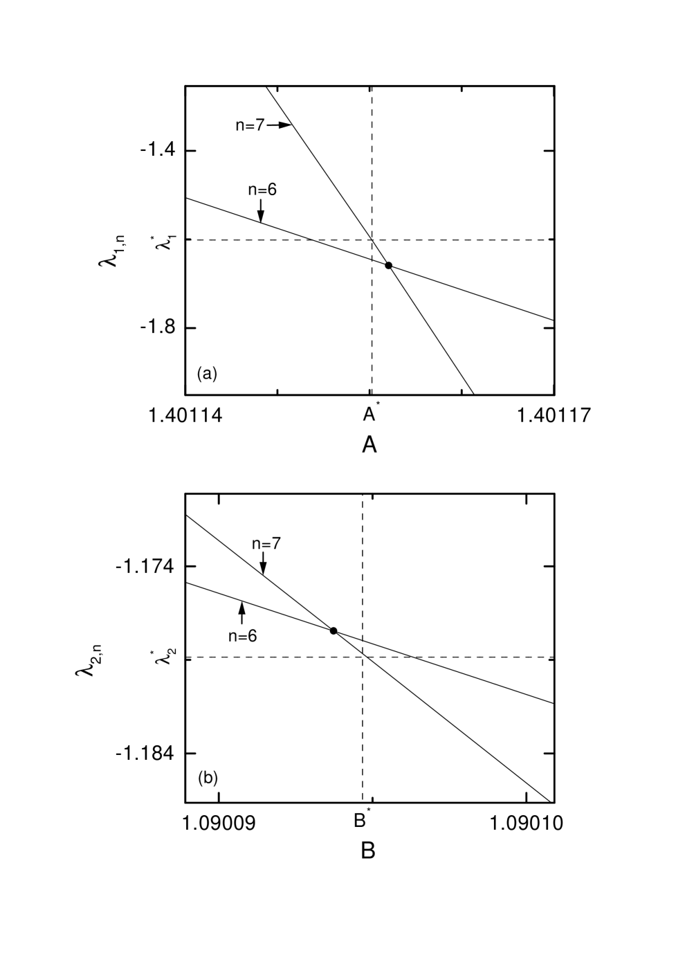
FIG. 3.: Plots of (a) the first stability multipliers $\lambda_{1,n}(A)$ versus $A$ and (b) the second stability multipliers $\lambda_{2,n}(A^{*}_{6},B)$ versus $B$ for the cases $n=6,7$. In (a), the intersection point, denoted by the solid circle, of the two curves $\lambda_{1,6}$ and $\lambda_{1,7}$ gives the point $(A^{*}_{6},\lambda_{1,6}^{*})$ of level $6$. As $n\rightarrow\infty$, $(A^{*}_{n},\lambda^{*}_{1,n})$ converges to its limit point $(A^{*},\lambda_{1}^{*})$. Similarly, in (b), the intersection point, denoted also by the solid circle, of the two successive curves $\lambda_{2,6}(A^{*}_{6},B)$ and $\lambda_{2,7}(A^{*}_{6},B)$ gives the point $(B^{*}_{6},\lambda_{2,6}^{*})$ of level $6$. As $n\rightarrow\infty$, $(B^{*}_{n},\lambda^{*}_{2,n})$ also approaches its limit point $(B^{*},\lambda_{2}^{*})$. For other details, see the text.

With increasing the level up to $n=15$, we numerically make the RG analysis of the bicritical behavior. We first solve Eq. (III B) and obtain the bicritical point $(A^{*}_{n},B^{*}_{n})$ of level $n$ and the pair of critical stability multipliers $(\lambda^{*}_{1,n},\lambda^{*}_{2,n})$ of level $n$. Next, we use the formulas of Eqs. (III B) and (III B) and obtain the parameter and orbital scaling factors of level $n$, respectively. These numerical RG results for the first and second subsystems are listed in Tables IV and V, respectively. Note that the accuracy in the numerical RG results is remarkably improved with the level $n$ and their limit values agree well with those obtained by a direct numerical method.

TABLE IV.: Sequences of the critical point, the first critical stability multiplier, the parameter and orbital scaling factors, $\{A^{*}_{n}\}$, $\{\lambda^{*}_{1,n}\}$, $\{\delta_{1,n}\}$ and $\{\alpha_{1,n}\}$, in the first subsystem. For comparison, we also list the results obtained by a direct numerical method in the last row.

$n$	$A^{*}_{n}$	$\lambda^{*}_{1,n}$	$\delta_{1,n}$	$\alpha_{1,n}$
6	1.401 155 189 088 929 1	-1.601 191 211 121 2	4.669 203 072 1	-2.502 620 459 5
7	1.401 155 189 092 133 2	-1.601 191 342 517 1	4.669 201 428 5	-2.502 845 988 3
8	1.401 155 189 092 048 4	-1.601 191 326 288 7	4.669 201 631 4	-2.502 894 652 0
9	1.401 155 189 092 050 7	-1.601 191 328 294 3	4.669 201 606 3	-2.502 905 037 7
10	1.401 155 189 092 050 6	-1.601 191 328 046 4	4.669 201 609 4	-2.502 907 267 8
11	1.401 155 189 092 050 6	-1.601 191 328 077 0	4.669 201 609 1	-2.502 907 744 9
12	1.401 155 189 092 050 6	-1.601 191 328 073 2	4.669 201 609 1	-2.502 907 847 2
13	1.401 155 189 092 050 6	-1.601 191 328 073 7	4.669 201 609 1	-2.502 907 869 1
14	1.401 155 189 092 050 6	-1.601 191 328 073 6	4.669 201 609 1	-2.502 907 873 8
15	1.401 155 189 092 050 6	-1.601 191 328 073 6	4.669 201 609 1	-2.502 907 874 8
	1.401 155 189 092 050 6	-1.601 191 328 073 6	4.669 201 609 1	-2.502 907 875 1

TABLE V.: Sequences of the critical point, the second critical stability multiplier, the parameter and orbital scaling factors, $\{B^{*}_{n}\}$, $\{\lambda^{*}_{2,n}\}$, $\{\delta_{2,n}\}$ and $\{\alpha_{2,n}\}$, in the second subsystem. For comparison, we also list the results obtained by a direct numerical method in the last row.

$n$	$B^{*}_{n}$	$\lambda^{*}_{2,n}$	$\delta_{2,n}$	$\alpha_{2,n}$
6	1.090 092 490 313	-1.177 467	2.395 07	-1.502 785
7	1.090 094 351 702	-1.178 671	2.393 58	-1.503 173
8	1.090 094 321 847	-1.178 625	2.393 59	-1.504 426
9	1.090 094 328 376	-1.178 649	2.393 10	-1.504 894
10	1.090 094 347 652	-1.178 820	2.392 80	-1.504 993
11	1.090 094 348 817	-1.178 844	2.392 81	-1.505 163
12	1.090 094 348 536	-1.178 830	2.392 78	-1.505 263
13	1.090 094 348 675	-1.178 847	2.392 74	-1.505 280
14	1.090 094 348 704	-1.178 856	2.392 73	-1.505 296
15	1.090 094 348 701	-1.178 853	2.392 73	-1.505 311
	1.090 094 348 701	-1.178 85	2.392 7	-1.505 318

IV Summary

We have studied the scaling behavior of period doublings near the bicritical point, corresponding to a threshold of chaos in both subsystems. For this bicritical case, a new type of non-Feigenbaum critical behavior appears in the second (response) subsystem, while the first (drive) subsystem is in the Feigenbaum critical state. Employing the truncation and eigenvalue-matching methods, we made the RG analysis of the bicritical behavior. For the case of the truncation method, we analytically obtained the fixed point, associated with the bicritical behavior, and its relevant eigenvalues. These analytic RG results are not bad as the lowest-order approximation. To improve the accuracy, we also employed the numerical eigenvalue-matching RG method, and obtained the bicritical point, the parameter and orbital scaling factors, and the critical stability multipliers. Note that the accuracy in the numerical RG results is improved remarkably with increasing the level $n$. Consequently, these numerical RG results agree well with the results obtained by a direct numerical method. The results on the bicritical behavior in the abstract system of unidirectionally-coupled 1D maps are also confirmed in the real system of unidirectionally-coupled oscillators [10].

REFERENCES

• [1] M. J. Feigenbaum, J. Stat.Β Phys.Β 19, 25 (1978); 21, 669 (1979).
• [2] Kaneko, Phys.Β Lett.Β A 111, 321 (1985); I. S. Aranson, A. V. Gaponov-Grekhov and M. I. Rabinovich, Physica D 33, 1 (1988); K. Kaneko, Physica D 68, 299 (1993); F. H. Willeboordse and K. Kaneko, Phys.Β Rev.Β Lett.Β 73, 533 (1994); F. H. Willeboordse and K. Kaneko, Physica D 86, 428 (1995); O. Rudzick and A. Pikovsky, Phys.Β Rev.Β E 54, 5107 (1996); J. H. Xiao, G. Hu and Z. Qu, Phys.Β Rev.Β Lett.Β 77, 4162 (1996); Y. Zhang, G. Hu and L. Gammaiton, Phys.Β Rev.Β E 58, 2952 (1998).
• [3] B. P. Bezruchko, V. Yu. Gulyaev, S. P. Kuznetsov, and E. P. Seleznev, Sov. Phys. Dokl. 31, 268 (1986).
• [4] A. P. Kuznetsov, S. P. Kuznetsov and I. R. Sataev, Int. J. Bifurcation and Chaos 1, 839 (1991).
• [5] J.-M. Mao and J. Greene, Phys. Rev. A 35, 3911 (1987); S.-Y. Kim and H. Kook, Phys.Β Lett.Β A 178, 258 (1993).
• [6] B. Derrida, A. Gervois and Y. Pomeau, J. Phys.Β A 12, 269 (1979); B. Derrida and Y. Pomeau, Phys.Β Lett.Β A 80, 217 (1980); B. Hu and J. M. Mao, Phys.Β Rev.Β A 25, 1196 (1982); 25, 3259 (1982); Phys.Β Lett.Β A 108, 305 (1985); J. M. Mao and R. H. G. Helleman, Phys.Β Rev.Β A 35, 1847 (1987); S.-Y. Kim and B. Hu, Phys.Β Rev.Β A 41, 5431 (1990).
• [7] B. P. Bezruhko, Yu. V. Gulyaev, O. B. Pudovochkin, and E. P. Seleznev, Sov. Phys. Dokl. 35, 807 (1991).
• [8] R. S. MacKay, Ph.Β D. thesis, Princeton University, 1982. See Eqs.Β 3.1.2.12 and 3.1.2.13.
• [9] O. E. R$\rm{\ddot{o}}$ssler, Phys. Lett. A 71, 155 (1979).
• [10] S.-Y. Kim and W. C. Lim (to be published).