Periodic orbit sum rules for billiards:
Accelerating cycle expansions

Abstract

We show that the periodic orbit sums for 2-dimensional billiards satisfy an infinity of exact sum rules. We test such sum rules and demonstrate that they can be used to accelerate the convergence of cycle expansions for averages such as Lyapunov exponents.

PACS: 03.20.+i, 03.65.Sq, 05.40.+j, 05.45.+b
keywords: cycle expansions, periodic orbits, dynamical zeta functions, sum rules, billiards.

1 Introduction

Periodic orbit theory is a powerful tool for description of chaotic dynamical systems [1, 2, 3]. However, as one is dealing with infinities of cycles, the formal theory is not meaningful unless supplemented by a theory of convergence of cycle expansions. For nice hyperbolic systems, the theory is well developed, and shows that exponentially many cycles suffice to estimate chaotic averages with super-exponential accuracy [4, 5, 6]. However, for generic dynamical systems with infinitely specified grammars and/or non-hyperbolic phase space regions, the convergence of the dynamical zeta functions and spectral determinants cycle expansions is less remarkable. The infinite symbolic dynamics problem is generic, and a variety of strategies for dealing with it have been proposed: stability truncations [7, 8], approximate partitions [9], noise regularization  [10] and even abandoning the periodic theory altogether [11].

Computation of periodic orbits for a given system is often a considerable investment, as locating exhaustively the periodic orbits of increasing length for flows in higher dimensions can be a demanding chore. It is therefore essential that the information obtained be used in an as effective way as possible. Here we propose a new, hybrid approach of combining cycle expansions with exact results for “nearby” averages, based on the observation that the periodic orbit sums sometimes satisfy exact sum rules.

Studies of convergence of cycle expansions, such as comparisons [12] of truncation errors of the dimension and the topological entropy for the Hénon attractor, indicate strong correlations in truncation errors for different averages. We propose to turn these correlations in our favour, by using the error known exactly by a sum rule to improve the estimate for a nearby average for which no exact result exist. Billiards provide a convenient, physically motivated testing ground for this idea. The approach is inspired by the formula (16) for mean free flight time in billiards, so well known to the Russian school that it went unpublished for decades [13]. In this paper we show that billiards obey an infinity of exact periodic orbit sum rules, and indicate how such rules might be used to accelerate convergence of cycle expansions.

The paper is organised as follows: sect. 2 is a brief summary of the theory of periodic orbit averaging. In sect. 3 we review the known exact sum rules for billiards, and then generalise them to an infinity of sum rules. In sect. 4 we present the conventional cycle expansion numerical results for our test system, the overlapping three-disk billiard. This system is hyperbolic and does not suffer from the intermittency effects that plague billiards such as the stadium and the Sinai billiards, but is still “generic” in the sense that its symbolic dynamics is arbitrarily complicated. In sect. 5 and appendix A we develop a method which utilizes the flow conservation sum rule to accelerate the convergence of cycle expansions, and apply the method to our test system.

2 Periodic orbit averaging

We start with a summary of the basic formulas of the periodic orbit theory - for details the reader can consult refs. [1, 3].

A flow ${\bf x}\rightarrow{{\bf f}^{t}({\bf x})},x\in{\cal M}$, is a continuous mapping ${\bf f}^{t}:{\cal M}\rightarrow{\cal M}$ of the phase space ${\cal M}$ onto itself, parameterised by time $t$. On a suitably defined Poincaré surface of section ${\cal P}$, the dynamics is reduced to a return map

$$x\rightarrow{f^{n}(x)}\hskip 28.45274ptx\in{\cal P}\,,$$ (1)

where $n$ is the “topological time”, the number of times the trajectory returns to the surface of section.

A dynamical zeta function [4] associated with the flow ${{\bf f}^{t}(x)}$ is defined as the product over all prime cycles $p$

$${1/\zeta}(z,{s},\beta)=\prod_{p}\left(1-t_{p}\right)\ ,\qquad t_{p}=t_{p}(z,{s},\beta)=\frac{1}{|\Lambda_{p}|}e^{\beta A_{p}-{s}{T_{p}}}z^{{n_{p}}}\,,$$ (2)

where ${T_{p}}$, ${n_{p}}$ and $\Lambda_{p}$ are the period, topological length and stability of prime cycle $p$, $A_{p}$ is the integrated observable $a(x)$ evaluated on a single traversal of cycle $p$

$$A_{p}=\left\{\begin{array}[]{ll}\displaystyle\int_{0}^{{T_{p}}}a\left({{\bf f}^{\tau}(x_{0})}\right)d\tau&\mbox{(flows)}\\ \displaystyle\sum_{k=0}^{{n_{p}}-1}a\left({f^{k}({x_{0}})}\right)&\mbox{(maps)}\\ \end{array}\right.\,x_{0}\in p\,,$$ (3)

where ${s}$ is a variable dual to the time $t$, $z$ is dual to the discrete “topological” time ${n}$, and $t_{p}(z,{s},\beta)$ is the weight of the cycle $p$.

Classical averages over chaotic systems are given by cycle expansions constructed from derivatives of dynamical zeta functions. By expanding the product (2) a dynamical zeta function  can be represented as a cycle expansion

$$1/\zeta = 1-\mathop{{\sum}^{\prime}}_{\pi}t_{\pi}$$

$$t_{\pi} = t_{\pi}(z,{s},\beta)=(-1)^{k_{\pi}+1}t_{p_{1}}t_{p_{2}}\dots t_{p_{k}}$$ (4)

$$= (-1)^{k_{\pi}+1}{1\over|\Lambda_{\pi}|}e^{\beta A_{\pi}-{s}{T_{\pi}}}z^{{n_{\pi}}}\,.$$

where the prime on the sum indicates that the sum is restricted to pseudocycles, built from all distinct products of non-repeating prime cycles weights. The pseudocycle topological length, period, integrated observable, and stability are

$${n_{\pi}} = {n_{p_{1}}}+\ldots+{n_{p_{k}}}\,,\qquad{T_{\pi}}={T_{p_{1}}}+\ldots+{T_{p_{k}}}$$

$$A_{\pi} = A_{p_{1}}+\ldots+A_{p_{k}}\,,\qquad\Lambda_{\pi}=\Lambda_{p_{1}}\Lambda_{p_{2}}\cdots\Lambda_{p_{k}}\,,$$ (5)

where $k=k_{\pi}$ is the number of involved prime cycles. For economy of notation we shall usually omit the explicit dependence of $1/\zeta$ and $t_{p}$ on ($z$, ${s}$, $\beta$) whenever the dependence is clear from the context.

Truncation of the dynamical zeta function with respect to the topological length ${n_{\pi}}\leq N$ will be indicated by a subscript

$${1/\zeta}_{N}(z,{s},\beta)=1-\mathop{{\sum}^{\prime}}_{{n_{\pi}}\leq N}t_{\pi}\,.$$ (6)

If the system bounded (such that no trajectories escape), the dynamical zeta function (2) has a leanding zero at ${1/\zeta}(1,0,0)=0$. Expressing this condition in terms of the cycle expansion (4) we find that any bound system satisfies the flow conservation sum rule [3]:

$${1/\zeta}(1,0,0)=1-\mathop{{\sum}^{\prime}}_{\pi}(-1)^{k_{\pi}+1}{1\over|\Lambda_{\pi}|}=0\,.$$ (7)

The cycle expansions for the phase space average of observable $a(x)$ are given by either the integral over the natural measure, or by the cycle expansions

$$\mbox{flows: }\left\langle{a}\right\rangle_{\mbox{\footnotesize{flow}}} = \int_{\cal M}a(x)\rho(x)d{x}=\frac{\left\langle{A}\right\rangle_{\zeta}}{\left\langle{T}\right\rangle_{\zeta}}$$ (8)

$$\mbox{maps: }\left\langle{a}\right\rangle_{\mbox{\footnotesize{map}}} = \int_{\cal P}a(x)\rho(x)dx=\frac{\left\langle{A}\right\rangle_{\zeta}}{\left\langle{n}\right\rangle_{\zeta}},$$ (9)

where $\rho$ denotes the natural measure. As we shall show in (16) below, the averages computed from the two representations of dynamics are related by the mean free flight time.

The cycle expansions required for the evaluation of periodic orbit averages (8) and (9) are given by derivatives of the dynamical zeta function with respect to $\beta$, ${s}$ and $z$

$$\left\langle{A}\right\rangle_{\zeta} = \frac{\partial}{\partial\beta}{1/\zeta}(1,0,0)=\mathop{{\sum}^{\prime}}_{\pi}(-1)^{k_{\pi}+1}A_{\pi}/|\Lambda_{\pi}|$$ (10)

$$\left\langle{T}\right\rangle_{\zeta} = -\frac{\partial}{\partial s}{1/\zeta}(1,0,0)=\mathop{{\sum}^{\prime}}_{\pi}(-1)^{k_{\pi}}T_{\pi}/|\Lambda_{\pi}|$$ (11)

$$\left\langle{n}\right\rangle_{\zeta} = \frac{\partial}{\partial z}{1/\zeta}(1,0,0)=\mathop{{\sum}^{\prime}}_{\pi}(-1)^{k_{\pi}+1}n_{\pi}/|\Lambda_{\pi}|\,.$$ (12)

3 Periodic obit sum rules for billiards

We start by reviewing the mean free flight time sum rule for billiards discussed by Chernov in ref. [13].

In a $d$-dimensional billiard, a point particle moves freely inside a domain $Q$, scattering elastically off its boundary $\partial Q$. The billiard flow $f^{t}$ on ${\cal M}=Q\times S^{d-1}$ (where $S$ is the unit sphere of velocity vectors) has a natural Poincaré surface of section associated with the boundary

$${\cal P}=\partial{{\cal M}}=\left\{\left(q,v\right)\in{\cal M}:q\in\partial Q\mbox{ and }v\cdot n(q)\geq 0\right\}$$ (13)

where $n(q)$ is the inward normal vector to the boundary at $q$, defined everywhere except at the singular set $\partial{{\cal M}}^{*}$ of nondifferentiable points of the boundnary (corners,cusps,etc). In what follows we shall restrict the discussion to (two-dimensional) billiards.

Assume that the particle has unit mass and moves with unit velocity, $p_{1}^{2}+p_{2}^{2}=1$. The cartesian coordinates and their conjugate momenta for the full phase space ${\cal M}$ of the billiard are

$${\bf x}=\left(q_{1},q_{2},p_{1},p_{2}\right)=\left(q_{1},q_{2},\sin\phi,\cos\phi\right)\,.$$

Let the Poincaré map be the boundary-boundary map $f:\partial{{\cal M}}\to\partial{{\cal M}}$, and parametrise the boundary $\partial{{\cal M}}$ by the Birkhoff (area preserving) coordinates

$$x=\left(s,p_{s}\right),\qquad p_{s}=\sin\theta,$$

where $s$ is the arclength measured along the boundary, $\theta$ is the scattering angle measured from the outgoing normal, and $p_{s}$ is the component of the momentum parallel to the boundary. Both the area of the billiard $A=|Q|$ and its perimeter length $L=|\partial Q|$ are assumed finite. Let $\tau(x)$ be the time of flight until the next collision. The continuous trajectory is parametrised by the Birkhoff coordinates together with a time coordinate $0<t<\tau(x)$ measured along the ray emanating from the boundary point $x=(s,p_{s})$.

The period of a cycle $p$ is the sum of the finite free-flight segments

$${T_{p}}=\sum_{k=0}^{{n_{p}}-1}\tau\left(f^{k}(x_{0})\right),$$

where $x_{0}=(s_{0},p_{s,0})$ is any of the collision points in cycle $p$. The mean free flight time is the average time of flight between successive bounces off the billiard boundary. It can be expressed either as a time average

$${\bar{\tau}}(x_{0})=\lim_{n\rightarrow\infty}{1\over n}\sum_{i=0}^{n-1}\tau(f^{i}(x_{0})),$$

or, as a phase space average

$$\left\langle{\tau}\right\rangle=\int_{{\cal P}}\tau(x)d{\mu}(x),$$ (14)

where $d{\mu}(x)=ds\;dp_{s}/\int_{{\cal P}}ds\;dp_{s}$ is the natural measure. For Hamiltonian flows like the billiard flow considered here this is simply the Lebesgue measure. If the billiard is ergodic, the time average is defined and independent of $x_{0}$ for almost all $x_{0}$. In order to find an exact expression for the phase space average $\left\langle{\tau}\right\rangle$, compute the integral over the entire phase space of the billiard,

$$\int_{\cal M}\delta(1-p_{1}^{2}-p_{2}^{2})dq_{1}dq_{2}dp_{1}dp_{2}=2\pi A$$

and recompute the same thing in the Birkhoff coordinates,

$$\int\delta(1-p_{1}^{2}-p_{2}^{2})dq_{1}dq_{2}dp_{1}dp_{2} = \int_{{\cal P}}dsdp_{s}\int_{t=0}^{\tau(x)}dt=\int_{{\cal P}}\tau(x)dsdp_{s}$$ (15)

$$= \left\langle{\tau}\right\rangle\int_{{\cal P}}dsdp_{s}=2L\left\langle{\tau}\right\rangle,$$

where $L$ is the circumference of the billiard. Hence the mean free flight time is a purely geometric property of the billiard,

$$\left\langle{\tau}\right\rangle=\pi\frac{A}{L},$$ (16)

the ratio of its perimeter to its area. The relation is a consequence of the Liouville measure being constant and apply to any billiard regardless of whether its phase space is mixed or not. For ergodic systems the periodic orbit theory gives a cycle expansion formula (9) for the mean free flight time

$$\left\langle{\tau}\right\rangle=\frac{\left\langle{T}\right\rangle_{\zeta}}{\left\langle{n}\right\rangle_{\zeta}}.$$ (17)

If we know $\left\langle{\tau}\right\rangle$ this formula enables us to relate any discrete time average (9) computed from the map to the continuous time averages (8) computed on the flow. They are linked by the mean free flight time formula

$$\left\langle{a}\right\rangle_{map}=\left\langle{a}\right\rangle_{flow}\left\langle{\tau}\right\rangle.$$ (18)

In what follows we will restrict our attention to map averages, and omit the subscript $\left\langle{\ldots}\right\rangle_{map}\rightarrow\left\langle{\ldots}\right\rangle$.

As the next example of a periodic orbit sum rule, consider the case of the observable being the transverse momentum change at collision, $a=2\cos\theta$. The corresponding sum rule is called the pressure sum rule because it is related to the pressure exerted by the particle on the billiard boundary.

The average pressure is given by the relation $P=F/\left|\partial Q\right|$, where $F$ is the time average of momentum change, that is the force the particle exerts against the boundary. The momentum change per bounce equals twice the transverse momentum at the collision, so the average force per bounce is

$$\left\langle{F}\right\rangle_{map}=\int_{{\cal P}}2p_{\perp}(x)d{\mu}(x)=\frac{1}{\int_{\cal P}dsdp_{s}}\int_{\partial Q}\int_{-\pi/2}^{\pi/2}2\cos\theta\cos\theta d\theta ds=\frac{\pi}{2}\,.$$ (19)

Hence the pressure for a flow becomes

$$\left\langle{P}\right\rangle_{flow}=\frac{\left\langle{F}\right\rangle_{map}}{L\left\langle{\tau}\right\rangle}=\frac{1}{2A}.$$ (20)

The exact averages (16), (20) apply to billiards of any shape, ergodic or not. As both the mean free path and pressure can be calculated by means of cycle expansions, these relations leads to exact billiard sum rules.

Now we note that as the Liouville invariant measure of the map is constant, any average of an observable $a(x)$, defined in terms of $\partial{{\cal M}}$ coordinates $x=(s,p_{s})$ can be expressed in terms of a simple integral. For each such observable we obtain an exact periodic orbit sum rule

$$\left\langle{a}\right\rangle=\frac{\left\langle{A}\right\rangle_{\zeta}}{\left\langle{n}\right\rangle_{\zeta}}=\int_{{\cal P}}a(x)d\mu(x).$$ (21)

Surprisingly enough, this uncountable infinity of sum rules seems not to have been noted in the literature.

The formula (21) does not allow for analytical computation of every average we want to compute in a billiard. Consider the simplest nontrivial average worth study in billiards, the diffusion coefficient

$$\left\langle{D}\right\rangle=\frac{1}{2d}\frac{1}{\left\langle{n}\right\rangle_{\zeta}}\frac{\partial^{2}}{\partial\beta^{2}}\left.({1/\zeta})\right|_{\beta=0}.$$ (22)

It requires evaluation of a second derivative of the relevant dynamical zeta function, this means that two-point correlations of the observable along cycles will enter the averaging formulas, so the average can not be computed from one iterate of the map.

Another quantity of interest is the Lyapunov exponent. Let $\Lambda(x_{0},n)$ is the largest eigenvalue of the Jacobian of the $n$th iterate of the map. The (largest) Lyapunov exponent is defined as

$$\lambda=\lim_{n\rightarrow\infty}\frac{1}{n}\log|\Lambda(x_{0},n)|\,.$$

The cycle expansion formulas in sect. 2 compute

$$\lambda=\lim_{n\rightarrow\infty}\frac{1}{n}\int d\rho(x)\log|\Lambda(x,n)|\,,$$ (23)

that is, a combination of time and phase space averages. Note that if $\Lambda(x_{0},n)$ is multiplicative, $\Lambda(x_{0},n)=\prod_{k=0}^{n-1}\Lambda(f^{k}(x_{0}))$, then the integral in (23) is independent of $n$: setting $n=1$, reduces the problem to one iterate of the map. This is the case for 1-dimensional maps. However in most cases the invariant measure $\rho(x)$ is not known a priori, and there is no simple exact formula for the average.

For billiards the invariant density is known but the expanding stability eigenvalue $\Lambda(x_{0},n)$ is not multiplicative along an arbitrary trajectory, , and the integral in (23) is dependent on $n$. It is possible to derive a multiplicative evolution operator for this purpose  [14]. However, for the purpose at hand the naive cycle expansion formulas still apply, because $\Lambda(x_{0},n)$ is multiplicative for repeats of periodic orbits. By defining the cycle weight

$$e^{\beta A_{p}}=|\Lambda_{p}|^{\beta}$$

the cycle expansion for the Lyapunov exponent is given by

$$\left\langle{\lambda}\right\rangle=\frac{\left\langle{\ln{|\Lambda|}}\right\rangle_{\zeta}}{\left\langle{n}\right\rangle_{\zeta}}$$ (24)

So even though Lyapunov only requires computation of two first order derivatives of the dynamical zeta function, it requires $n$-point correlations to all orders and cannot be computed by a sum rule.

In the case when (18) the Lyapunov exponent of the flow to the Lyapunov exponent of the corresponding Poincaré return map, the relation is known as the Abramov’s formula  [15].

4 Three overlapping disks billiard

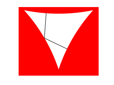
Figure 1: The overlapping 3-disk billiard. A point-like particle moves inside the billiard bouncing specularly off the boundary. Shown is a cycle of topological length 4.

We will test the above sum rules on cycle expansions for a concrete system, the overlapping 3-disk billiard. This billiard consists of three disks of radius $a$ centered on the corners of an equilateral triangle with sides $R$. There is a finite enclosure (see fig. 1) between the disks if $\sqrt{3}<R/a\leq 2$. This enclosure defines the billiard domain $Q$. One of the limits $R/a\rightarrow\sqrt{3}$ corresponds to the integrable equilateral triangle billiard. The other limiting case $R/a=2$ exhibits intermittency with infinite sequences of periodic orbits whose periods $T_{p}$ accumulate to finite limits, and where stabilities fall off as some power $n_{p}^{\alpha}$, where $n_{p}$ is the topological length.

The $C_{3v}$ symmetry of the billiard enables us to work in the fundamental domain [16]. The fundamental domain is one 6th slice of the billiard domain, fenced in by the symmetry axes of the billiard. In what follows we are only interested in the lowest eigenvalue and therefore we restrict our computations to the fully symmetric $A_{1}$ subspace. The fundamental domain symbolic dynamics is binary, but is not of the finite subshift type; its full specification would require an infinity of pruning rules of arbitrary length.

The mean free flight time (16) for the overlapping 3-disk billiard can be found by geometric considerations,

$$\left\langle{\tau}\right\rangle=\pi\frac{R^{2}/4\sqrt{3}-a^{2}\theta-Rr/2}{2a\theta},$$ (25)

where $r=\sqrt{a^{2}-(R/2)^{2}}$ and $\theta=\pi/6-\arcsin(r/a)$. We shall set $a=1$ throughout this paper, and parameterise the billiard by the center-to-center distance $R$. All our numerical tests are done for $R=1.9$. Results for this parameter value, as well as for $R=1.85$ are shown in table 1.

$R$	$\left\langle{\tau}\right\rangle$	$\left\langle{\lambda}\right\rangle$	$\lambda_{\mbox{num}}$	$L\left\langle{P}\right\rangle$	# cycles
1.85	0.102	0.523		1.57	342
1.9	0.1401	0.6036	0.60363	1.570	525

Table 1: The mean free flight time $\left\langle{\tau}\right\rangle$ , the average pressure $P$ , and the best estimate of the Lyapunov exponent $\lambda$ computed by cycle expansion as function of the 3-disk center-to-center separation $R$ used in our numerical tests, with disk radius fixed to $a=1$. For $R=1.9$ a numerically computed Lyapunov reference value obtained by direct simulation using $10^{10}$ bounces is displayed. The total numbers of the fundamental domain prime cycles used in the cycle expansion computations are also indicated.

Fig. 2 illustrates the convergence of finite topological length cycle expansions for the flow conservation sum rule (7) and for the mean free flight time sum rule (17). As the exact result is known, we plot the logarithm of the error as function of the truncation length N.

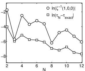
Figure 2: Convergence of cycle expansions: Deviation of cycle expansions truncated to the topological length $N$ from exact sum rules for ($\circ$) flow conservation (7) and ($\Box$) mean free flight time (17).

The overall exponential convergence reflects the existence of a gap, the dynamical zeta functions are analytic beyond $z=1$. The “irregular” oscillations in fig. 2 are typical for systems with complicated symbolic dynamics. For systems with finite subshift symbolic dynamics the oscillations ceases when the cutoff $N$ exceeds the longest forbidden substring and if the full spectral determinant is used, super-exponential convergence sets in [12].

One should note the coincidence of the peaks and dips of the two curves. This type of correlations between coefficients between different power series will be important in the following.

5 Utilizing exact sum rules

We shall illustrate the utility of exact sum rules in accelerating the convergence of cycle expansions by applying flow conservation sum rule to the problem of computing the mean free flight time (16). As we already have the exact formula for this average, we will be able to compute the exact error in the various estimates and compare them. We will then apply the same technique to evaluate the Lyapunov exponent, for which no exact formula exists.

The idea is to use the flow conservation sum rule (7) to improve the numerator and denominator of (17) separately.

We begin by the denominator. The general problem is to find a good estimate of the derivative $F^{\prime}(z_{0})$ at the first root $F(z_{0})=0$ of a function given by a power series $F(z)=\sum_{k=0}^{\infty}b_{k}z^{k}$ where the coefficients are known only up to order $N$

$$F_{(N)}(z)=\sum_{k=0}^{N}b_{k}z^{k},$$ (26)

and we know (appendix A) that a good estimate is given by

$$F^{\prime}(z_{0})\approx F^{\prime}_{(N)}(z_{0})-\frac{N+1}{z_{0}}F_{(N)}(z_{0}).$$ (27)

We argue in appendix A that the error in the above estimate is suppressed compared to the error of the estimate $F^{\prime}_{(N)}(z_{0})$ by a factor $q$ whose asymptotic behaviour is

$$q\sim 1/N.$$ (28)

The improved estimate of the derivative of the zeta function (12) thus reads

$$\left\langle{n}\right\rangle_{\zeta,acc}\approx\left\langle{n}\right\rangle_{\zeta,(N)}-(N+1)\zeta^{-1}_{(N)}(1,0,0).$$ (29)

The continuous time average by invoking the sum rule (7) is similar to the previous one but ${1/\zeta}(1,{s},0)=0$ is now a Dirichlet series in ${s}$. The basic idea is to start by expanding the zeta function around some point ${s}={s}_{0}$

$${1/\zeta}(1,{s},0)=1-\mathop{{\sum}^{\prime}}_{\pi}\frac{(-1)^{k_{\pi}-1}}{|\Lambda_{\pi}|}e^{-{s}T_{\pi}}$$

$$=1-\mathop{{\sum}^{\prime}}\frac{(-1)^{k_{\pi}-1}}{|\Lambda_{\pi}|}e^{-s_{0}T_{\pi}}\sum_{k=0}^{\infty}\frac{(s_{0}-s)^{k}T_{\pi}^{k}}{k!}.$$

Since we have only a finite number of of pseudocycles at our disposal, it is not meaningful to consider high powers $k$ in the above Taylor series. So we truncate the series

$${1/\zeta}_{(N,M)}(1,{s},0) = 1-\mathop{{\sum}^{\prime}}_{\pi:n_{\pi}\leq N}\frac{(-1)^{k_{\pi}-1}}{|\Lambda_{\pi}|}e^{-s_{0}T_{\pi}}\sum_{k=0}^{M}\frac{(s_{0}-s)^{k}T_{\pi}^{k}}{k!}$$ (30)

$$= 1-\sum_{k=0}^{M}\frac{\left\langle{T^{k}}\right\rangle_{\zeta,(N)}}{k!}(s_{0}-s)^{k}\,.$$

where

$$\left\langle{T^{k}}\right\rangle_{\zeta,(N)}=\mathop{{\sum}^{\prime}}_{\pi:n_{\pi}\leq N}(-1)^{k_{\pi}-1}\frac{e^{-s_{0}T_{\pi}}T_{\pi}^{k}}{|\Lambda_{\pi}|}$$

is the $k$th moment of the average cycle time. The sets of periodic orbits going into the calculation are still being truncated according to their topological length. This finite Taylor series is the analogue of the truncated function $F_{(N)}(z)$ treated above; $s=0$ corresponds to $z=1$, and $s=s_{0}$ to $z=0$. We can use (27) and write down the improved estimate

$$\left\langle{T}\right\rangle_{\zeta,acc}\approx\left\langle{T}\right\rangle_{\zeta,(N)}-\frac{M+1}{s_{0}}\zeta^{-1}_{(N,M)}(1,0,0)$$ (31)

However there is now an additional complication due to the fact that not all available $\left\langle{T^{k}}\right\rangle_{\zeta}$ are exact. So how should we choose $s_{0}$ and $M$? We choose $s_{0}$ to lie somewhere in the range $1/T_{max}<s_{0}<1/T_{min}$ where the $T_{min}$ and $T_{max}$ are the smallest and largest period in the sample for a particular topological length cutoff $N$.

The next question is, for a given $s_{0}$, what is the number of accurate coefficients $\left\langle{T^{k}}\right\rangle_{\zeta,(N)}/k!$? We see from (30) that pseudocycles are suppressed with their length according to the function $T^{k}\exp(-s_{0}T)$ having its maximum at $T=k/s_{0}$. So the coefficients with $k\ll s_{0}T_{max}$ can be expected to be accurate. However, as the majority of cycles have periods close to $T_{max}$ we want to make use of the information they carry. We have found it preferable to include a large number of fairly accurate coefficients rather than a small number of very accurate ones. So we choose the maximum power $M$ to be given by the average cycle length

$$M=s_{0}\left.{\overline{T}}_{p}\right|_{{n_{p}}=N-1}$$

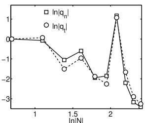
Figure 3: The error suppression factor for ($\Box$) maps and for ($\circ$) flows, applied to the 3-disk system with $R=1.9$. Here we have used an extrapolated value from the cycle expansion as the best asymptotic estimate. Both error suppressions display the estimated error decrease and demonstrate that the sum rules do improve convergence.

The error of the improved estimate is suppressed compared to the error of the traditional estimate by factor we call $q$, see appendix A. This $q$-factor is plotted in fig. 3. It decreases (apart from oscillations) as the estimated $N^{-1}$ error suppression derived for maps.

The calculation of the integrated observable amounts to evaluating the $\beta$ derivatives of the dynamical zeta functions. The role of $\beta$ is completely analogous to that of $s$. With $\beta$ viewed as a complex variable, the dynamical zeta function ${1/\zeta}(1,0,\beta)$ is a Dirichlet series in $\beta$ and the above methods can be used to compute $\frac{\partial}{\partial\beta}{1/\zeta}(1,0,0)$. Here similar criteria apply to $\beta_{0}$ and $N$ as for (31) : $\beta_{0}$ close to $1/A_{min}$ and $M=\beta_{0}\left.{\overline{A}}_{p}\right|_{{n_{p}}=N-1}$.

5.1 Improvement on the averages

So far we have improved the numerator and the denominator of (17) and (9) separately. The errors of both are suppressed by a factor $q\approx O(1/N)$ compared to unaccelerated estimates. We have also seen (fig. 3) that, both before and after resummation, their behavior versus the cutoff $N$ are highly correlated. So it is not obvious how the resulting average should be improved, indeed it is not clear whether it is improved at all.

The accelerated cycle expansion for an observable $a(x)$ using our method is

$$\left\langle{a}\right\rangle_{acc}=\frac{\left\langle{A}\right\rangle_{\zeta,acc}}{\left\langle{n}\right\rangle_{\zeta,acc}},$$ (32)

and the error suppression, the $q$-factor for the observable $a(x)$ is

$$q_{a}=\frac{\left\langle{a}\right\rangle_{acc}-\left\langle{a}\right\rangle_{exact}}{\left\langle{a}\right\rangle-\left\langle{a}\right\rangle_{exact}}.$$ (33)

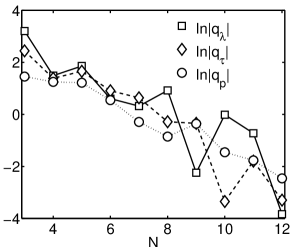
Figure 4: The error suppression factor (33) for : ($\Diamond$) The accelerated mean free flight timesum rule. ($\circ$) pressure sum rule. ($\Box$) The Lyapunov exponent. At topological length 12 the accuracy of the accelerated Lyapunov exponent has reached the best estimate from direct numerical simulation (see Table 1).

We compute this $q$ factor numerically for three different averages:

• The mean free flight time $\left\langle{\tau}\right\rangle$ by (17). The exact result is given by (16).

• The average force $\left\langle{F}\right\rangle_{map}$ by (19), associated with the pressure sum rule. The exact result is given by (20).

• The Lyapunov exponent by (24). The reference value of the Lyapunov exponent is obtained by numerical simulation, see Table 1.

The results are summarized in fig. 4. The accelerated cycle expansions are clearly better than the standard cycle expansions. The error suppression factors appear to decrease exponentially, and therefore the acceleration techniques has for the 3-disk system increased the correlation between the expansions leading to a faster convergence for the averages.

6 Conclusion

In this paper we have achieved two objectives: (i) We have derived an infinite number of exact periodic orbit sum rules for billiards (21). Such sum rules enable us to make exact computations of some statistical averages for billiards, such as the mean free flight time (16) and pressure (20). (ii) We have derived the improved estimate (31) which combines the flow conservation sum rule (7) with the cycle expansions. In order to measure the convergence acceleration, we have introduced the error suppression factor (33) that gauges the improvement of the accelerated cycle expansions relative to the unaccelerated ones. We thus demonstrate that exact sum rules can be used to accelerate convergence for observables for which no exact results exist, see fig. 4.

A challenge for the future is to utilize such infinities of sum rules for billiards in the classical applications (other than the Lyapunov exponent studied here), as well as in the semi-classical applications of periodic orbit theory.

This work was supported by the Swedish Natural Science Research Council (NFR) under contract no. F-AA/FU 06420-312 and no. F-AA/FU 06420-313. PD thanks NORDITA for partial support. SFN thanks PD and KTH for hospitality.

Appendix A Resummation of power series

Consider a function $F(z)$ given by a power series, where only a finite number of coefficients are known.

$$F_{(N)}(z)=\sum_{k=0}^{N}b_{k}z^{k}.$$ (34)

We assume that $F(z_{0})=0$ for some $z_{0}$ and we wish to estimate the first derivative $F^{\prime}(z_{0})$ (and possibly higher derivatives) as accurately as possible. The general problem is to transform the Taylor series around $z=0$ into a Taylor series around $z=z_{0}$, and extract the desired coeficients. This is done by the ansatz

$$\sum_{k=0}^{N}b_{k}z^{k}=\sum_{i=1}^{N+1}a_{i}(z-z_{0})^{i}+O(z^{N+1})$$ (35)

Note that the sum rule is built into this ansatz by setting $a_{0}=0$. Our aim is to determine $F^{\prime}(z_{0})=a_{1}$. We keep the number of known and unknown coefficients equal so that the system of equations is solvable.

Expanding the right hand side (35) binomially

$$\sum_{i=0}^{N}b_{i}z^{i}=\sum_{i=1}^{N+1}a_{i}\sum_{j=0}^{i}z^{j}(-z_{0})^{i-j}{i\choose j}+O(z^{N+1})$$

we obtain the linear system of equations

$$b_{j}=\sum_{\max(j,1)}^{N+1}{i\choose j}(-1)^{i-j}a_{i},\qquad 1\leq i\leq N+1\mbox{ and }0\leq j\leq N.$$ (36)

In order to transform this to matrix equations where all indices range from $1$ to $n\equiv N+1$ we define vectors

$$({\bf b})_{i}=z_{0}^{i-1}b_{i-1},\qquad({\bf a})_{i}=z_{0}^{i}a_{i}\ \ ,$$ (37)

and rewrite (36) as

$${\bf b}={\bf M}{\bf a},\qquad({\bf M})_{ij}={j\choose i-1},\qquad 1\leq i,j\leq n(-1)^{j-i+1}.$$ (38)

We use a convention that ${n\choose m}=0$ if $m$ is out of range. This system may readily be solved. Define the matrix ${\bf L}$ by

$$({\bf L})_{ij}=\left\{\begin{array}[]{cc}1&i\geq j\\ 0&i<j\end{array}\right.$$ (39)

Then

$$({\bf LM})_{ij}=(-1)^{i+j+1}{j-1\choose i-1}\rightarrow({\bf LM})^{-1}_{ij}=-{j-1\choose i-1},$$

and the explicit solution is

$${\bf a}=({\bf LM})^{-1}{\bf Lb}$$ (40)

In particular

$$({\bf a})_{1} = -n\;({\bf b})_{1}-(n-1)\;({\bf b})_{2}-\ldots-1\;({\bf b})_{n}=-\sum_{k=1}^{n}(n-k+1)({\bf b})_{k}$$

$$z_{0}a_{1} = ({\bf a})_{1}=-\sum_{k=0}^{N}(n-k)z_{0}^{k}b_{k}=z_{0}F^{\prime}_{(N)}(z_{0})-(N+1)F_{(N)}(z_{0})$$ (41)

So our improved estimate of $F^{\prime}(z_{0})$ is

$$F^{\prime}(z_{0})\approx a_{1}=F^{\prime}_{(N)}(z_{0})-(N+1)z_{0}^{-1}F_{(N)}(z_{0})$$ (42)

The error is suppressed by a factor

$$q=\frac{F^{\prime}_{N}(z_{0})-nz_{0}^{-1}\;F_{N}(z_{0})-F^{\prime}(z_{0})}{F^{\prime}_{N}(z_{0})-F^{\prime}(z_{0})}=\frac{\sum_{k=n}^{\infty}(k-n)b_{k}}{\sum_{k=n}^{\infty}kb_{k}}$$ (43)

To get this on a more handy form we use summation by parts, that is, we define

$$1/q=1+\frac{ns_{n}}{\sum_{k=n+1}^{\infty}s_{k}},\qquad s_{k}=\sum_{j=k}^{\infty}b_{j}$$ (44)

If $F(z)$ is the spectral determinant for a $d$-dimensional Axiom-$A$ map the coefficients of the power series expansion are super-exponentially bounded

$$C_{a}\Lambda^{-n^{1+1/d}}_{a}<|b_{n}|<C_{b}\Lambda^{-n^{1+1/d}}_{b}$$ (45)

where $1<\Lambda_{b}<\Lambda_{a}$. Assuming moreover that the signs of the coefficients settle down to some periodic pattern, one can show that the error supression factor has the following asymptotic behaviour

$$q\sim n^{-(1+1/d)}$$ (46)

In this paper we focus on a hyperbolic systems whose symbolic dynamics cannot be finitely specified. In that case the bound on the coefficients is exponential

$$C_{a}\Lambda^{-n}_{a}<|b_{n}|<C_{b}\Lambda^{-n}_{b},$$ (47)

and nothing can be said about the signs, as they can oscillate in a completely irregular fashion [17]. It seems difficult to obtain proper bounds on $q$ in a general setting. In the case at hand we can only provide a qualified guess on the decrease of the error supression factor

$$q\sim n^{-1}$$ (48)

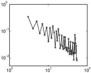
Figure 5: Error suppression factor (33) (y-axis) versus truncation in topological length N(x-axis) for the tent map (with a “typical” slope value $\Lambda$).

Some evidence for this behavior can be provided by the tent map

$$F(x)=\left\{\begin{array}[]{c}\Lambda x\mbox{ for }x<\frac{1}{2}\\ -\Lambda(x-1)\mbox{ for }x\geq\frac{1}{2}\\ \end{array}\right..$$ (49)

The expansion rate is uniform but complete symbolic dynamics is lacking in the generic case. In fig. 5 we plot the q-factor for the tent map for a randomly chosen parameter versus $N$. It conforms with the predicted $1/N$ behavior.

The ansatz (35) used here is the simplest conceivable and it led to very simple formulas. The only requirement is that the dynamical zeta function is analytic in a disk $z\leq R$ where $R>1$. This excludes strongly intermittent systems where a more refined ansatz is needed[18]. If one has some explicit knowledge of the nature of the leading singularity of the dynamical zeta function, one can taylor a more specific ansatz.

References

- [1] P. Gaspard, Chaos, Scattering and Statistical Mechanics (Cambridge University Press, New York 1998).
- [2] M.C. Gutzwiller, Chaos in Classical and Quantum Mechanics (Springer, New York 1990).
-
[3]
P. Cvitanović et al.,
Classical and Quantum Chaos,
http://www.nbi.dk/ChaosBook/ (Niels Bohr Institute, Copenhagen 1998). - [4] D. Ruelle, Ergod. The. and Dynam. Sys. 2, 99 (1976).
- [5] H.H. Rugh, Nonlinearity 5, 1237 (1992).
- [6] P. Cvitanović, P.E. Rosenqvist, H.H. Rugh, and G. Vattay, CHAOS 3, 619 (1993).
- [7] C.P. Dettmann and G.P. Morriss, Phys. Rev. Lett. 78, 4201 (1997).
- [8] P. Dahlqvist and G. Russberg, J. Phys. A 24, 4763 (1991).
-
[9]
K.T. Hansen,
Symbolic Dynamics in Chaotic Systems,
Ph. D. thesis (University of Oslo 1993).
http://www.nbi.dk/CATS/papers/khansen/ - [10] P. Cvitanović, C.T. Dettmann, R. Mainieri and G. Vattay, J. Stat. Phys (1998), to appear.
- [11] P. Cvitanović, J. Rolf, K. Hansen and G. Vattay, Nonlinearity 11, 1233 (1998)
- [12] R. Artuso, E. Aurell and P. Cvitanović, Nonlinearity 3, 361 (1990).
- [13] N. Chernov, J. Stat. Phys. 88, 1 (1997).
- [14] P. Cvitanović and Gabor Vattay, Phys. Rev. Lett. 71, 4138 (1993).
- [15] L. M. Abramov, Dokl. Akad. Nauk. SSSR 128, 873, (1959).
- [16] P. Cvitanović and B. Eckhardt, Nonlinearity 6, 277 (1993).
- [17] P. Dahlqvist, J. Math. Phys. 38, 4273 (1997).
- [18] P. Dahlqvist, J. Phys. A 30, L351 (1997).