[

Thermostatting by deterministic scattering

Abstract

We present a mechanism for thermalizing a moving particle by microscopic deterministic scattering. As an example, we consider the periodic Lorentz gas. We modify the collision rules by including energy transfer between particle and scatterer such that the scatterer mimics a thermal reservoir with arbitrarily many degrees of freedom. The complete system is deterministic, time-reversible, and provides a microcanonical density in equilibrium. In the limit of the disk representing infinitely many degrees of freedom and by applying an electric field the system goes into a nonequilibrium steady state.

PACS numbers: 05.20.-y, 05.45.+b, 05.60.+w, 05.70.Ln, 44.90.+c

]

Thermostatting is a mechanism by which the internal energy of a many-particle system, and thus its temperature, are kept constant although there is a flux of energy through the system as, e.g., induced by external fields, or by imposing temperature or velocity gradients [3]. In order to study nonequilibrium transport in fluids by computer simulations, Evans, Hoover, Nosé and others developed methods of thermostatting by introducing a fictitious frictional force into the microscopic equations of motion [4, 5], modeling the interaction of particles with a thermal reservoir. This force is chosen to be velocity dependent in a way that the (total or kinetic) energy of the particles remains constant and that, in an equilibrium situation, the system approaches microcanonical or canonical distributions of the phase space variables. In contrast to stochastic thermostats [3, 6, 7], this class of dynamical systems is completely deterministic and time-reversible, making them suitable models to study the connection between microscopic reversibility and macroscopic irreversibility. This led to interesting new relations between statistical physics and dynamical systems theory [4, 5, 8], especially between transport coefficients and Lyapunov exponents [9, 10, 11, 12], and between irreversible entropy production and phase space contraction [7, 10, 13, 14, 15]. On the other hand, employing these friction coefficients for creating nonequilibrium steady states is physically somewhat obscure, because the equations of motion are fundamentally modified. It has been shown that the resulting dynamical systems belong to some new class of generalized Hamiltonian systems [4, 5, 16], but the problem still remains whether the relations mentioned above rely on having specifically this class of systems, or whether they are of a general nature [7, 17, 18, 19]. Much recent work [19, 20, 21] has been devoted to deal with this question, and to relate this way to model nonequilibrium states to the one initiated by Gaspard, where nonequilibrium is induced by appropriate boundary conditions in spatially extended systems [18, 22].

One of the simplest examples of a dynamical system in which thermostatting by a velocity-dependent friction coefficient has been applied is the field driven periodic Lorentz gas. The classical periodic Lorentz gas, where a point particle scatters elastically at hard disks arranged on a triangular lattice, has been the subject of many investigations and serves as a standard model in the field of chaos and transport [18, 19, 20, 21, 22]. In the field driven case an electric field acts on the moving particle and a thermostat keeps the energy of the particle constant at all times [5, 9, 12, 14, 23, 24, 25, 26]. For unit mass and unit charge of the particle the equations of motion read $\mbox{\boldmath$\dot{r}$}=\mbox{\boldmath$v$}\>,\>\mbox{\boldmath$\dot{v}$}=\mbox{\boldmath$\varepsilon$}-\zeta(\mbox{\boldmath$v$})\mbox{\boldmath$v$}\>,$ plus the geometric constraints induced by the disks. $r$ and $v$ represent position and velocity of the moving particle, $\varepsilon$ is the electric field, and $\zeta(\mbox{\boldmath$v$})$ stands for the friction coefficient which, by requiring energy conservation, is determined to be $\zeta(\mbox{\boldmath$v$})=\mbox{\boldmath$\varepsilon\cdot v$}/v^{2}$. This set-up provides an example of a so-called Gaussian thermostat [4, 5, 8].

In this Letter we propose an alternative mechanism of deterministic, time-reversible thermostatting that does not appeal to such a frictional force. We shall implement this mechanism by adapting the geometry of the periodic Lorentz gas, in which it suffices to consider one scatterer in an elementary cell supplemented by periodic boundary conditions, as depicted in Fig. 1 (a). For the spacing between two neighboring disks at disk radius $R=1$ we choose, following the literature [9, 12, 25, 26], $w\simeq 0.2361$, ensuring that no particle can move collision-free for infinite time. Fig. 1 (b) defines the relevant variables for the collision process. At the collision we express the velocity $v$ of the colliding particle in local polar coordinates

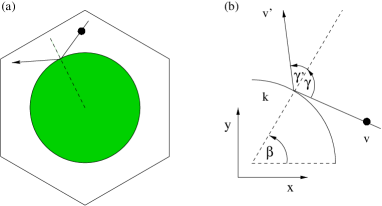
FIG. 1.: (a) Elementary cell of the periodic Lorentz gas on a triangular lattice. (b) Definition of the relevant variables to describe the collision process.

$(\gamma,v)$, where $\gamma$ is the angle of incidence and $v$ the absolute value of the velocity. The dashed variables indicate the respective values after the collision. We also introduce the angle $\beta$, which determines the position of the colliding particle at the disk. For an elastic collision, as in case of the original Lorentz gas, one has $(\gamma,v)=(\gamma^{\prime},v^{\prime})$. In contrast to this, we propose to include an energy transfer between particle and disk, which, viewed in this way, serves as a momentum- and energy-reservoir. We do this by introducing an additional velocity variable $k$ associated to the disk and by allowing that $\gamma\neq\gamma^{\prime}$. We require that the energy is conserved at the collision, $v^{2}+k^{2}=v^{\prime 2}+k^{\prime 2}=2E$, where $E$ is the total energy of the system. Thus, the collision process in velocity space is still effectively defined by the dynamics of two variables for which we take $(\gamma,v)$. Using this setup, one can construct a model where the disk rotates with $k$ as an angular velocity [27]. By keeping the component of $v$ perpendicular to the disk fixed and allowing only exchange of energy via the tangent component, the collision process effectively reduces to the one of two colliding masses on a line. Requiring energy and momentum conservation yields for the scattering rules a two-dimensional piecewise linear map. As a drastic simplification of such a model, but keeping important dynamical properties like time-reversibility, a deterministic dynamics, and the dynamical instability induced by the disk geometry, we choose here our collision rules according to a simple baker map [8, 28, 29]. We apply it on the respective Birkhoff coordinate of the ingoing angle, $\sin|\gamma|$, as its $x$-coordinate, and on $v$ in the range of $0\leq v\leq\sqrt{2E}$ as its $y$-coordinate. To ensure that the system is time-reversible, the forward baker acts if $0\leq\gamma\leq\pi/2$, and its inverse if $-\pi/2\leq\gamma<0$. The angle $\gamma^{\prime}$ always goes to the respective other side of the normal, as shown in Fig. 1 (b). For $\gamma\geq 0$ this gives

$$M(\sin|\gamma|,v)=\left\{\begin{array}[]{r@{,}l@{\:,\:}l}(2\sin|\gamma|&v/2)\hfil\>,\>&\sin|\gamma|\leq 0.5\\ (2\sin|\gamma|-1&(v+1)/2)\hfil\>,\>&\sin|\gamma|>0.5\\ \end{array}\right.$$ (1)

and vice versa for $\gamma<0$. As for $k^{\prime}$, it is obtained from energy conservation. To avoid any symmetry breaking induced by this combination of forward and backward baker, we alternate their application in $\gamma$ with respect to the position $\beta$ of the colliding particle on the circumference[30].

The above setting leads to a well-defined scattering system with three degrees of freedom. As it stands, however, it does not satisfy the microcanonical distribution, since the energy is not equipartitioned between all degrees of freedom, corresponding to a distribution $\rho(v_{x},v_{y},k)$ not being unifom on the energy shell $v_{x}^{2}+v_{y}^{2}+k^{2}=2E$. We incorporate this essential feature by amending the microscopic scattering rules, as given by the baker, in the most straightforward way: As a starting point, we calculate the projection of the microcanonical density $\rho(v_{x},v_{y},k)=\delta(2E-v_{x}^{2}-v_{y}^{2}-k^{2})$ onto $v$ yielding $\rho(v)=v/\sqrt{2E(2E-v^{2})}$. We want that our system approaches this density in the long time limit. Let $\rho_{map}(v)$ be the probability density for $v$ at the moment of the collision corresponding to a respective Poincaré surface of section, in contrast to the probability density of the time-continuous system, which we may denote with $\rho_{cont}(v)$. During the free flight the particle cannot change its velocity, and thus $\rho_{map}(v)$ and $\rho_{cont}(v)$ are simply related via the average time the particle travels between two collisions with velocity $v$. This average time plays the role of a weighting factor leading to

$$\rho_{cont}(v)=\frac{c}{v}\rho_{map}(v)\quad,$$ (2)

where $c$ is a constant to be fixed by normalization. Thus, we want that the map which determines the collision rules generates an invariant velocity distribution $\rho_{cont}^{*}(v)\equiv\rho(v)$ corresponding to

$$\rho_{map}^{*}(v)=\frac{2v^{2}}{\pi E\sqrt{2E-v^{2}}}\quad.$$ (3)

However, the invariant density of the baker map is simply $\rho^{*}(x_{B},y_{B})=\rho^{*}(x_{B})\rho^{*}(y_{B})=1$. Therefore, we define a conjugate map which produces the desired density by including a transformation $y_{B}=Y(v)$, where $y_{B}$ is the actual baker variable. This transformation must be continuous and invertible, as defined by conservation of probability [28],

$$\rho^{*}(y_{B})|dy_{B}|=\rho_{map}(v)|dv|\quad.$$ (4)

$Y(v)$ can then immediately be computed to

$$Y(v)=-\frac{v}{\pi E}\sqrt{2E-v^{2}}+\frac{2}{\pi}\arcsin\frac{v}{\sqrt{2E}}$$ (5)

with $0\leq v\leq\sqrt{2E}\>,\>0\leq Y(v)\leq 1$. If we write $x_{B}=X(\gamma)=\sin|\gamma|$, the full collision rules are thus given by

$$(\gamma^{\prime},v^{\prime})=(X^{-1},Y^{-1})\circ M\circ(X(\gamma),Y(v))\quad.$$ (6)

Computer simulations show that a Lorentz gas with these collision rules is microcanonical in both its position and momentum coordinates in phase space [27].

We now inquire how the above ideas can be used to mimic the interaction of a moving particle with a thermal reservoir. For this purpose we associate arbitrarily many degrees of freedom to the disk which could be related, e.g., to different lattice modes in a crystal, as mechanisms for dissipating energy from a colliding particle. For sake of simplicity we do not distinguish here between all the individual velocities in the reservoir. Instead, we pretend that the particle interacts instantaneously with all $(d-2)$ velocity components $k_{j}$ of the reservoir via an absolute reservoir velocity $k=\sqrt{k_{1}^{2}+k_{2}^{2}+\ldots+k_{d-2}^{2}}$, to which we identify the disk velocity. We want that the projected densities of the accessible variables $(v_{x},v_{y},k)$ be generated from the microcanonical distribution of the full $d$-dimensional system. In particular, the projection of the microcanonical distribution $\rho_{d}(v_{x},v_{y},k_{1},k_{2},\ldots,k_{d-2})=\delta(2E-v_{x}^{2}-v_{y}^{2}-\sum_{j=1}^{d-2}k_{j}^{2})$ onto $\rho_{d}(v)$ can be calculated for $d>2$ to [31]

$$\rho_{d}(v)=(d-2)(2E)^{-\frac{d-2}{2}}v(2E-v^{2})^{\frac{d-4}{2}}\quad.$$ (7)

Using the equipartition theorem $E/d=T/2$ with $T$ the temperature and a Boltzmann constant $k_{B}=1$, and taking the limit $d\to\infty$, this expression reduces to the Maxwellian distribution $\rho_{\infty}(v)=v/T\exp(-v^{2}/(2T))$. Choosing $\rho_{cont,d}^{*}(v)\equiv\rho_{d}(v)$ according to Eq. (7) and using Eq. (2) determines the corresponding density $\rho_{map,d}^{*}(v)$ of the Poincaré section. The transformation $Y_{d}(v)$ which yields $\rho_{map,d}^{*}(v)$ can then be calculated from Eq. (4) [27]. In the limit of $d\to\infty$, $Y_{\infty}(v)$ becomes especially simple and reads

$$Y_{\infty}(v)=-\sqrt{\frac{2}{\pi T}}ve^{-v^{2}/(2T)}+\mbox{erf}\left(\frac{v}{\sqrt{2T}}\right)$$ (8)

with $0\leq v\leq\infty\>,\>0\leq Y(v)\leq 1$. Computer simulations show that a periodic Lorentz gas with these collision rules approaches projected densities in $(v_{x},v_{y},k)$ which are identical to the ones obtained from a uniform distribution on the energy shell in $(v_{x},v_{y},k_{1},k_{2},\ldots,k_{d-2})$ [27]. The temperature $T$ of the equilibrium system is unambiguously defined via equipartitioning of energy as it enters into Eq. (8). Notice the complementarity between our approach and the procedure adopted when using stochastic boundary conditions [6, 7, 32].

We are now ready to set up a nonequilibrium situation by taking the system as defined in equilibrium for $d\to\infty$ and by switching on an electric field parallel to the $x$-axis. This field affects the velocity of the moving particle. However, since the particle is a small subsystem in a large reservoir, and since we have built in a mechanism of equipartitioning of energy, the particle is still getting thermalized by our scattering rules with a temperature determined by the temperature $T$ of the reservoir. In fact, computer simulations show that the system approaches a nonequilibrium steady state with kinetic energy and conductivity fluctuating around constant mean values [27]. That such a nonequilibrium steady state exists according to our scattering mechanism is the central result of our Letter.

In the following, we illustrate some important characteristics of this state by results obtained from computer simulations. Fig. 2 demonstrates that for small enough field strength and high enough temperature the energy of the system is still approximately equipartitioned between $<v^{2}>-<v_{x}>^{2}$ and the reservoir. Fig. 3 depicts the conductivity $\sigma(\varepsilon)=<v_{x}>/\varepsilon$ with respect to the field strength $\varepsilon$. The strong decrease of $\sigma(\varepsilon)$ indicates that the system is in a highly nonlinear regime. Ohm’s law may be suspected to hold only at very small field strengths

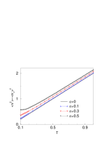
FIG. 2.: Relation between average velocity squared in the frame moving with the current, $<v^{2}>-<v_{x}>^{2}$, and temperature $T$ for the infinite dimensional model. Equipartitioning of energy would imply $<v^{2}>-<v_{x}>^{2}=2T$.

$\varepsilon\ll 0.1$ [14, 33], however, in this regime reliable numerical results are difficult to get. The broadest fluctuations on smaller scales are beyond numerical uncertainties and may be reminiscent to the strong irregularities as they occur in the conductivity of the Gaussian Lorentz gas [9, 23, 24, 25, 26]. Unfortunately, it is not clear how to compare the conductivities of these two models quantitatively, since the choice of temperature in the Gaussian model is somewhat ambiguous by a factor of two [14]. Fig. 4 (a),(b) show Poincaré plots of $(\beta,\sin\gamma)$ at the collisions. In (b) the deterministic baker has been replaced by a random number generator such that the system completely loses its memory at each collision. Fig. (a) indicates the existence of a fractal attractor, analogously to the one found in the Gaussian Lorentz gas [9, 25, 34], whereas in (b) the fractal structure is lost due to the stochasticity of the boundary conditions. Fig. 4 (c) should be compared to the analogous diagram obtained from the Lorentz gas with a Gaussian thermostat [5, 24, 35]. In case of our model, there is no indication of a pruning-induced “bifurcation scenario” or an ergodic breakdown like in the Gaussian version. The same holds for other choices of Poincaré sections in phase space.

It would be interesting to compare our approach in more detail to the one based on frictional forces. For this purpose, a Lorentz gas with a so-called Nosé-Hoover thermostat, where the particle velocity fluctuates around a mean value [9], would be a more adequate model to compare with, but we are not aware that such a model has been studied. It would also be important to compute Lyapunov exponents and fractal dimensions of the phase

FIG. 3.: Conductivity $\sigma(\varepsilon)$ as it varies with field strength $\varepsilon$. The curve consists of 90 data points, the numerical uncertainty of each point is less than $5\cdot 10^{-4}$.

FIG. 4.: (a),(b) Poincaré section of $(\beta,\sin\gamma)$ defined in Fig. 1 at the moment of the collision for field strength $\varepsilon=1$. In (a) the baker map of Eq. (1) has been used, in (b) the baker has been replaced by a random number generator. (c) Poincaré section of $\beta$ at the moment of the collision for varying field strength $\varepsilon$.

space densities for our model. This would enable to test the status of recently proposed connections between statistical physics and dynamical systems quantities as discussed in Refs. [12, 13, 14, 23, 24].

Our method has recently been applied to thermostat an interacting many-particle system of hard disks under shear [7], and with a temperature gradient, at the boundaries, where it leads to a connection between deterministic thermostats and thermalization at stochastic boundaries [32]. It would also be interesting to use it as a simple model for inelastic scattering in granular material, instead of employing velocity-dependent restitution coefficients [36].

We are indebted to P.Gaspard and Chr.Wagner for many important hints. R.K. thanks the DFG for financial support, K.R. thanks the European Commisssion for a TMR grant under contract no. ERBFMBICT96-1193.

REFERENCES

- [1]
- [2] Electronic address: rklages@ulb.ac.be.
- [3] see, e.g., M. Allen and D. Tildesley, Computer Simulation of Liquids (Clarendon Press, Oxford, 1987).
- [4] D. Evans and G. Morriss, Statistical Mechanics of Nonequilibrium Liquids, (Academic Press, London, 1990); W. G. Hoover, Computational Statistical Mechanics (Elsevier, Amsterdam, 1991); S. Nosé, in Computer Simulation in Material Science, edited by M. Meyer and V. Pontikis (Kluwer Academic Publishers, Netherlands, 1991), pp. 21–41.
- [5] G. Morriss and C. Dettmann, p. 321 of Ref. [21].
- [6] J. Lebowitz and H. Spohn, J. Stat. Phys. 19, 633 (1978).
- [7] N. Chernov and J. Lebowitz, Phys. Rev. Lett. 75, 2831 (1995); N. Chernov and J. Lebowitz, J. Stat. Phys. 86, 953 (1997); C. Dellago and H. Posch, ibid 88, 825 (1997).
- [8] J.R. Dorfman, An Introduction to Chaos in Non-Equilibrium Statistical Mechanics (Cambridge Univ. Press, Cambridge, 1999).
- [9] B. Moran and W. Hoover, J. Stat. Phys. 48, 709 (1987).
- [10] H. Posch and W. Hoover, Phys. Rev. A 38, 473 (1988).
- [11] D. Evans, E.G.D. Cohen, and G. Morris, Phys. Rev. A 42, 5990 (1990).
- [12] W. N. Vance, Phys. Rev. Lett. 69, 1356 (1992).
- [13] B. L. Holian, W. Hoover, and H. Posch, Phys. Rev. Lett. 59, 10 (1987).
- [14] N. Chernov, C. Eyink, J. Lebowitz, and Y. Sinai, Phys. Rev. Lett. 70, 2209 (1993); Comm. Math. Phys. 154, 569 (1993).
- [15] J. Vollmer, T. Tél, and W. Breymann, Phys. Rev. Lett. 79, 2759 (1997); W. Breymann, T. Tél, and J. Vollmer, p. 396 of Ref. [21]; T. Gilbert and J.R. Dorfman (unpublished).
- [16] P. Choquard, p. 350 of Ref. [21].
- [17] G. Nicolis and D. Daems, p. 311 of Ref. [21].
- [18] P. Gaspard, Chaos, Scattering, and Statistical Mechanics (Cambridge Univ. Press, Cambridge, 1998).
- [19] Microscopic Simulations of Complex Hydrodynamic Phenomena, edited by M. Mareschal and B. L. Holian (Plenum, New York, 1992).
- [20] The Microscopic Approach to Complexity in Non-Equilibrium Molecular Simulations, Vol. 240 of Physica A, edited by M. Mareschal (Elsevier, Amsterdam, 1997).
- [21] Chaos and Irreversibility, Vol. 8 of Chaos, edited by T. Tél, P. Gaspard and G. Nicolis (American Institute of Physics, College Park, 1998).
- [22] P. Gaspard and G. Nicolis, Phys. Rev. Lett. 65, 1693 (1990); P. Gaspard and J.R. Dorfman, Phys. Rev. E 52, 3525 (1995).
- [23] A. Baranyai, D. Evans, and E.G.D. Cohen, J. Stat. Phys. 70, 1085 (1993).
- [24] J. Lloyd, M. Niemeyer, L. Rondoni, and G. Morriss, Chaos 5, 536 (1995).
- [25] C. Dellago, L. Glatz, and H. Posch, Phys. Rev. E 52, 4817 (1995); W. Hoover and H. Posch, p. 366 of Ref. [21].
- [26] C. Dettmann and G. Morriss, Phys. Rev. Lett. 78, 4201 (1997).
- [27] K. Rateitschak, R. Klages, and G. Nicolis (unpublished).
- [28] E. Ott, Chaos in Dynamical Systems (Cambridge University Press, Cambridge, 1993).
- [29] We note that our thermostatying mechanism works as well with any other two-dimensional map, provided it is area-preserving and chaotic [32].
- [30] When is odd (even) we take the forward (backward) baker for and vice versa the corresponding backward (forward) baker for .
- [31] M. Kac, Probability and Related Topics in the Physical Sciences (Interscience, New York, 1959); N. van Kampen, Stochastic Processes in Physics and Chemistry (North Holland, Amsterdam, 1992).
- [32] C. Wagner, R. Klages, and G. Nicolis (unpublished).
- [33] N. van Kampen, Physica Norvegica 5, 279 (1971).
- [34] W. Hoover and B. Moran, Phys. Rev. A 40, 5319 (1989).
- [35] J. Lloyd, L. Rondoni, and G. Morriss, Phys. Rev. E 50, 3416 (1994).
- [36] T. Aspelmeier, G. Giese, and A. Zippelius, Phys. Rev. E 57, 857 (1998).