Improving the false nearest neighbors method with graphical analysis

Abstract

We introduce a graphical presentation for the false nearest neighbors (FNN) method. In the original method only the percentage of false neighbors is computed without regard to the distribution of neighboring points in the time-delay coordinates. With this new presentation it is much easier to distinguish deterministic chaos from noise. The graphical approach also serves as a tool to determine better conditions for detecting low dimensional chaos, and to get a better understanding on the applicability of the FNN method.

I Introduction

One of the main tasks of time series analysis is to determine from a given time series the basic properties of the underlying process, such as nonlinearity, complexity, chaos etc. Among the most widely used approaches is state space reconstruction by time delay embedding [1]. After this step has been taken one can calculate correlation dimensions, various entropy quantities and estimates for Lyapunov exponents. The crucial problem is how to select a minimal embedding dimension for the pseudo phase-space. If the embedding dimension is too small, one cannot unfold the geometry of the (possible strange) attractor, and if one uses a too high embedding dimension, most numerical methods characterizing the basic dynamical properties can produce unreliable or spurious results.

The false-nearest-neighbors (FNN) algorithm [2, 3, 4] is one of the tools that can be used to determine the number of time-delay coordinates needed to reconstruct the dynamics. In this method one forms a collection

$${\bf y}(k)=[x(k),x(k+1),\dots,x(k+d-1)]$$ (1)

of $d$-dimensional vectors for a given time delay (here normalized to 1), $x(1),x(2),\dots,x(N)$ is a scalar time series. If the number $d$ of time-delay coordinates in (1) is too small, then two time-delay vectors ${\bf y}(k)$ and ${\bf y}(l)$ may be close to each other due to the projection rather than to the inherent dynamics of the system. When this is the case, points close to each other may have very different time evolution, and actually belong to different parts of the underlying attractor.

In order to determine the sufficient number $d$ of time-delay coordinates one next looks at the nearest neighbor of each vector (1) with respect to the Euclidean metric. We denote the nearest neighbor of ${\bf y}(k)$ by ${\bf y}(n(k))$. We then compare the “$(d+1)$”st coordinates of ${\bf y}(k)$ and ${\bf y}(n(k))$, e.g., $x(k+d)$ and $x(n(k)+d)$. If the distance $|x(k+d)-x(n(k)+d)|$ is large the points ${\bf y}(k)$ and ${\bf y}(n(k))$ are close just by projection. They are false nearest neighbors and they will be pulled apart by increasing the dimension $d$. If the distances $|x(k+d)-x(n(k)+d)|$ are predominantly small, then only a small portion of the neighbors are false and $d$ can be considered a sufficient embedding dimension.

In the FNN algorithm [2, 3, 4] the neighbor is declared false if

$$\frac{|x(k+d)-x(n(k)+d)|}{\|{\bf y}(k)-{\bf y}(n(k))\|}>R_{tol},$$ (2)

or if

$$\frac{\|{\bf y}(k)-{\bf y}(n(k))\|^{2}+[x(k+d)-x(n(k)+d)]^{2}}{R_{A}^{2}}>A_{tol}^{2},$$ (3)

where

$$R_{A}^{2}=\frac{1}{N}\sum_{k=1}^{N}[x(k)-\overline{x}]^{2},$$ (4)

and $\overline{x}$ is the mean of all points. The parameter $R_{tol}$ in the first threshold test (1) is fixed beforehand, and in most studies it has been set to $10-20$. The second criterion (3) was proposed in order to provide correct diagnostics for noise and usually one takes $A_{tol}\approx 2$. If this test fails, then even the ($d+1$-dimensional) nearest neighbors themselves are far apart in the extended $d+1$ dimensional space and should be considered false neighbors.

Using tests (2) and (3) one can check all $d$-dimensional vectors in the data set, and compute the percentage of false nearest neighbors. By increasing the dimension $d$ this percentage should drop to zero or to some acceptable small number. In that case the embedding dimension is large enough to represent the dynamics.

This method works quite well with noise free data, and the percentage of false neighbors does not depend on the number of data points if it is sufficient. However, if data is corrupted with noise, the percentage of false nearest neighbors for a given embedding dimension increases as the amount of data is increased, and therefore a longer time series leads to erroneous false nearest neighbors as a result of noise corruption rather than of an incorrect embedding dimension. One possible solution to this problem is to modify the threshold test (2) to account for additional noise effects. For example, instead of test (2) the threshold could be determined by [5]

$$\frac{|x(k+d)-x(n(k)+d)|}{\|{\bf y}(k)-{\bf y}(n(k))\|}>R_{tol}+\frac{2\epsilon R_{tol}\sqrt{d}+2\epsilon}{\|{\bf y}(k)-{\bf y}(n(k))\|}.$$ (5)

Here the new parameter $\epsilon$ must be chosen properly. Obviously the optimal value for $\epsilon$ should be determined by the noise level but unfortunately we have usually very limited information on the amplitude of the noise in a given time series.

II Graphical representation of nearest neighbor distributions

Without a clear understanding of the distribution of neighboring points in the time delay coordinates the original test (2) or the modified test (5) cannot guarantee that we have reached a sufficient embedding dimension, even if the percentage of false nearest neighbors is low. We have therefore constructed a simple graphical presentation which simultaneously displays all essential features. The basic idea is that we show the distance $R_{\Delta}=|x(k+d)-x(n(k)+d)|$ as a function of the original distance $R_{d}=\|{\bf y}(k)-{\bf y}(n(k))\|$ for all $d$-dimensional vectors in the data set. The $x$-variable $R_{d}$ should be scaled with the normalization coefficient $\sqrt{d}$ in order to remove unessential changes in the graphs due to changes in the embedding dimension (see Appendix).

As the first example we have chosen the Henon system

$$X_{n+1}=1-1.4\,X_{n}^{2}+Y_{n},\quad Y_{n+1}=0.3\,X_{n}$$ (6)

The parameters of this system were selected from the chaotic region (the dimension of the attractor is $1.26$), and the total number of data points is $1000$. In Figure 1 we have plotted $(\tilde{R}_{d},R_{\Delta})$ pairs ($\tilde{R}_{d}=R_{d}/\sqrt{d}$) for all vectors ${\bf y}$. The displayed box size is $0.024\times 0.024$ units. Two distributions have also been presented in each graph: the $\tilde{R}_{d}$ distribution on the bottom part of the graphs, and the radial distribution plotted on the quarter arc. The embedding dimension $d$ is scanned from $1$ to $4$, and each set of four graphs is presented in four different cases where the amplitude of the additional uniformly distributed (measurement) noise is 0%, 0.1%, 1% and 10% of the total amplitude.

According to (2) a neighbor is false if it lies above the straight line going through the origin with slope $R_{tol}$. If we use the test (5) the line has the same slope but there is an intercept equal to the noise correction term (scaled with $\sqrt{d}$). Normally we must know the slope a priori but using these graphs it is not necessary. If there is no noise we clearly see that with the embedding dimension $>1$ all points lie in the sector determined by the $x$-axis and a line with slope angle well below 90 degrees. This important feature can be understood if we assume that the dynamics is given by

$$x(k+dT)=f(x(k),x(k+1),\dots,x(k+d-1)).$$ (7)

Then we can write

$$\big{|}x(k+d)-x(l+d)\big{|}\leq\big{\|}\nabla f(\xi)\big{\|}\big{\|}{\bf y}(k)-{\bf y}(l)\big{\|}$$ (8)

for some $\xi$, which implies that

$$\frac{R_{\Delta}}{R_{d}}\leq\big{\|}\nabla f(\xi)\big{\|}.$$ (9)

Therefore all points in the $(\tilde{R}_{d},R_{\Delta})$ plots must lie under a line which depends on the specific system. The limit (9) is true only when the embedding dimension is sufficient, and for noise it is never possible. If the time series includes some additional noise we see its effect as a blurred border line.

If the embedding dimension is too low the points cumulate close to the $y$-axis. The radial distribution plot confirms this result. If $d=1$ the distribution has significant values only with angles close to $90$ degrees but if $d>1$ the distribution is almost zero within a distinct range at high angles. The $\tilde{R}_{d}$ distribution is high only in the vicinity of zero. A small amount of noise (0.1%, the second row from the bottom in Figure 1) does not change the picture much.

If the level of additional noise is increased to 1% the points do not show as well formed pattern. Also the radial distribution is quite broad but it nevertheless has a clear zero range at high angles if the embedding dimension is $3$, which can be regarded as an indication of underlying chaotic (or at least deterministic) dynamics. The maximum of the $\tilde{R}_{d}$ distribution has clearly shifted towards large values which is typical for pure noise.

In the case of more noisy data (10% on the top row of Figure 1) the distribution of points is totally different. Increasing the embedding dimension does not really change the overall shape of the point distribution. The radial distribution is fairly even, and the $\tilde{R}_{d}$ distribution is well centered and its maximum shifts toward higher values when the embedding dimension is increased. (With this kind of distribution the modified test (5) does not really take noise effects into account.)

In Figure 2 we have presented corresponding graphs for the Lorenz system

$$\dot{X} = 16\,(Y-X)$$ (10)

$$\dot{Y} = X(45.92\,-Z)-Y$$ (11)

$$\dot{Z} = XY-4\,Z$$ (12)

using $10000$ data points and the sampling delay of $0.05$. For these parameter values the dimension of the attractor is $2.07$. Here we observe similar kind of behavior for various distributions as in the case of the Henon system. Since the true dimension of the attractor is greater than $2$, a clearly bounded sector pattern of points can only be seen in the graphs with embedding dimension $\geq 3$. For $d=2$ most of the points lie under a line with slope under $90$ degrees which is also reflected in the noticeable maximum of the radial distribution, and since there is only a small portion of points between this maximum and the $y$-axis we can estimate that the true dimension of the attractor is not much greater than $2$.

The effect of even a small amount of noise can be clearly seen in Figure 2. Already with 1% of noise the sector pattern has changed to a vertical one. This is shown clearly in the regression lines (corresponding to the first principal component of the points $(\tilde{R}_{d},R_{\Delta})$) plotted in Figure 2. In the two bottom rows the regression lines have a slope well below $90$ degrees, and this can be taken as evidence of deterministic dynamics. For the two top rows the regression line is almost vertical (see also Figure 3) indicating noise contamination. Furthermore we see that the $\tilde{R}_{d}$ distribution shows approximately Gaussian shape, which spreads out and moves further and further away from the origin as the noise level or embedding dimension increases. The radial distribution, on the other hand, moves closer to the $90$-degrees line as noise contamination increases, which means that the height/width ratio of the point distribution increases, and therefore that it is more and more difficult to predict the next point.

In the standard procedure noise effect are taken into account by the condition (3), which means that points outside a circle of radius $A_{tol}R_{A}$ are counted false (actually it is an ellipse, due to the scaling of $\tilde{R}_{d}$.) For Figures 2 and 4 this radius is 500 times the box size (and for figures 1 and 5 the factor is about 20). Although the boundary is quite far away one can imagine that higher levels of noise and higher embedding dimensions both increase the number of false neighbours, as has been reported [3, 4].

If the total number of data points of the preceeding system is decreased to $1000$ the graphs are not so simple to interpret (Figure 4). There is no significant difference between graphs with embedding dimension 2 and 3. As usual, reliable estimation of the underlying dynamical dimension requires a sufficient number of data points. However, by using this graphical representation we can nevertheless make a rough estimate on dimension even when only relatively few data points are available.

As a final example we have analyzed the Mackey-Glass system

$$\dot{X}=\frac{0.2\,X(t+31.8)}{1+[X(t+31.8)]^{10}}-0.1\,X(t)$$ (13)

using the sampling delay of 2. As the dimension of the attractor with these parameter values is about $3.6$, the embedding dimension must be at least 4. This can be seen in Figure 5: only in rightmost graph there is a clear sector type of pattern, and the radial distribution is zero over a nonzero range of angles near $90$ degrees.

III Conclusions

We have presented a graphical method to analyze time series in order to estimate the sufficient embedding dimension and the portion of additional noise. This tool consists of a $(\tilde{R}_{d},R_{\Delta})$ plot augmented with two distributions. Furthermore, the slope of the regression line of points in the $(\tilde{R}_{d},R_{\Delta})$ graphs can be used to recognize noise in deterministic systems.

The advantage of the present method is that even small amount of noise contamination can be distinguished from deterministic chaos. This also means that we now see how the problem of determining the correct embedding dimension becomes more difficult with even a small amount of noise, and that for a deterministic system where the proportion of noise is substantial one should use the conditions (2) or (5) with great caution. If the FNN algorithm is used to estimate the embedding dimension, our presentation should be used in parallel in order to get relevant and reliable results.

To summarize our method we present a list of guidelines on how to distinguish a deterministic time series from sources with noise:

The time series is produced by a deterministic system if:

1. the points in the $(\tilde{R}_{d},R_{\Delta})$ plot form a clear sector pattern with a zero radial distribution over a distinct range below $90$ degrees,

2. the $R_{d}$ distribution is centered close to zero,

3. the slope of the regression line is well below 90 degrees.

The noise level in the time series is substantial if:

1. the radial distribution is spread out over the whole range from 0 to 90 degrees,

2. the $R_{d}$ distribution has a clear maximum far away from zero,

3. the slope of the regression line is close to $90$ degrees.

Let $f$ be a function which has been sampled very densely. Then we can assume that the nearest neighbor of the $d$-dimensional vector is the vector that starts at the next (or previous) sample point

$$\bigl{(}f(t_{0}+\delta),f(t_{0}+2\delta),f(t_{0}+3\delta),\dots,f(t_{0}+d\delta)\bigr{)}.$$ (14)

The distance between these two points is therefore

$$R_{d} \,=\sqrt{\sum_{i=1}^{d}\bigl{(}f(t_{0}+i\delta)-f(t_{0}+(i-1)\delta)\bigr{)}^{2}}$$ (16)

$$\approx\sqrt{\sum_{i=1}^{d}\delta^{2}f^{\prime}(t_{0}+i\delta)^{2}}\approx\delta\sqrt{d}|f^{\prime}(t_{0})|,$$

where we have assumed that the function $f$ changes relatively slowly (or that it is linear). The distance between the targets is

$$R_{\Delta}=\big{|}f(t_{0}+\delta+1)-f(t_{0}+\delta)\big{|}\approx\delta\big{|}f^{\prime}(t_{0})\big{|},$$ (17)

and by combining the results (16) and (17) we conclude that the ratio of $R_{\Delta}/R_{d}$ is $1/\sqrt{d}$, and therefore is it reasonable in all cases to normalize this ratio with $\sqrt{d}$.

FIG. 1.: The target distance $R_{\Delta}$ as a function of the nearest neighbor distance $\tilde{R}_{d}$ for the Henon system (the dimension of the attractor is $1.26$). The total number of data points is $1000$. The rows correspond to indicated noise levels, the columns to indicated embedding dimensions.

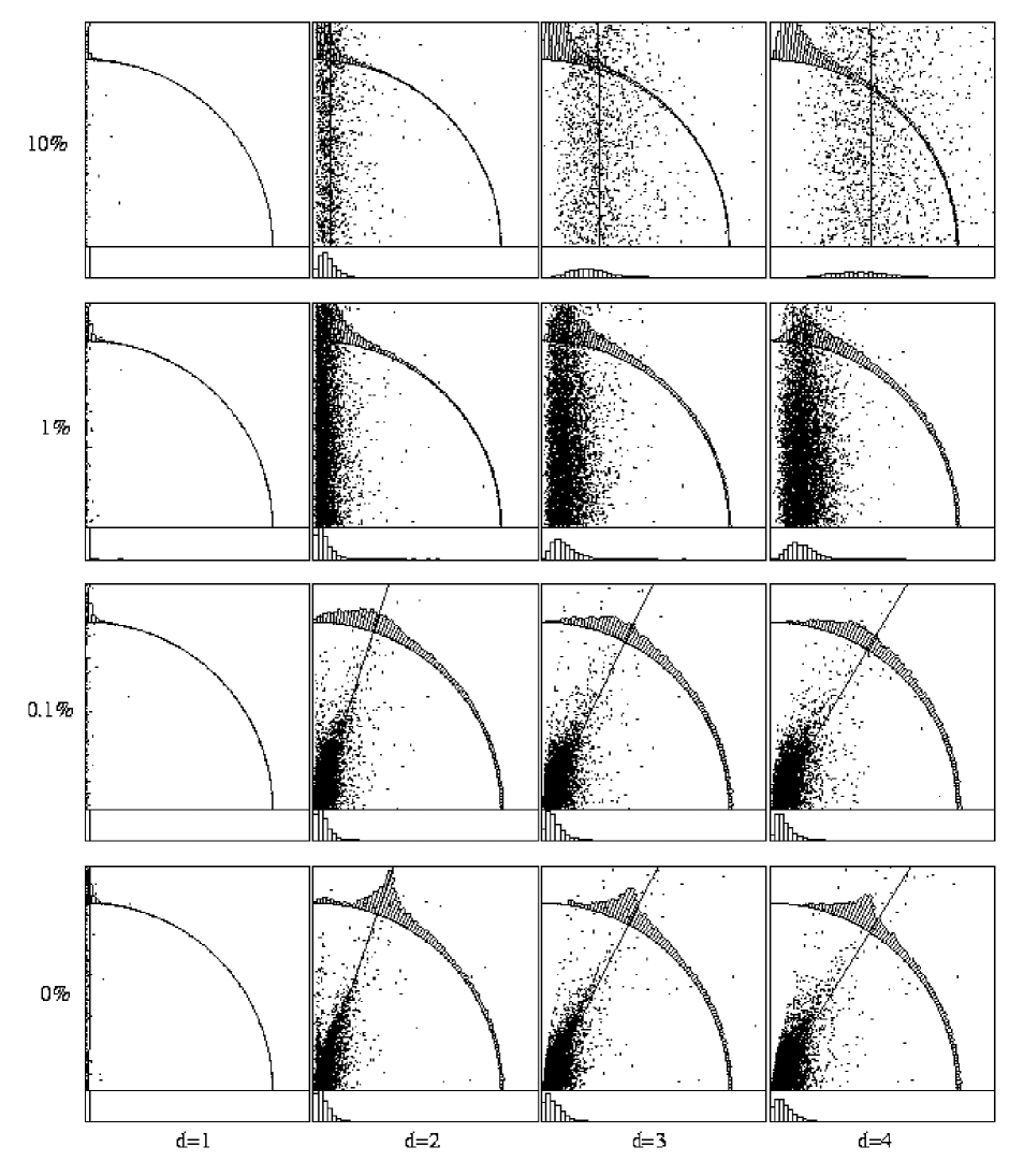
FIG. 2.: Same as in Figure 1 but for the Lorenz system (the dimension of the attractor is 2.06). The total number of data points is $10000$. The regression lines are also plotted on each graph. (We apologize for the low resolution of this figure, the original PostScript file was too big to store at this archive, but it is available at http://www.utu.fi/ hietarin/chaos/fnn.html.)

FIG. 3.: The slope of the regression line as a function of the embedding dimension for different percentage of noise taken from the graphs in Figure 2.

FIG. 4.: The same graphs as in the bottom row of Figure 2 but the total number of data points is only $1000$.

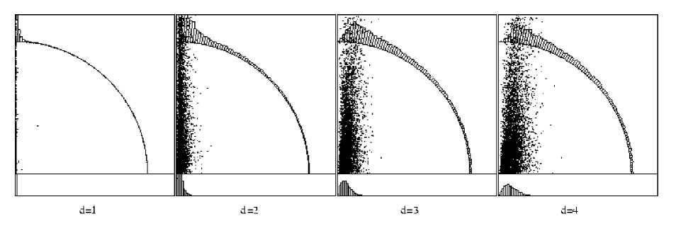
FIG. 5.: The target distance R_Δ as a function of the nearest neighbor distance $\tilde{R}_{d}$ for the Mackey-Glass system (the dimension of the attractor is $\sim 3.6$). The total number of data points is $10000$. (We apologize for the low resolution of this figure, the original PostScript file was too big to store at this archive, but it is available at http://www.utu.fi/ hietarin/chaos/fnn.html.)

REFERENCES

- [1] N.H. Packard, J.P. Crutchfield, J.D. Farmer, R.S. Shaw, Phys. Rev. Lett. 45, 712 (1980).
- [2] M.B. Kennel, R. Brown, H.D.I. Abarbanel, Phys. Rev. A 45, 3403 (1992)
- [3] H.D.I. Abarbanel, R.Brown, J.J. Sidorowich, L.S. Tsimring, Rev. Mod. Phys. 65, 1331 (1993).
- [4] H.D.I. Abarbanel, M.B. Kennel, Phys. Rev. E 47, 3057 (1993).
- [5] C. Rhodes, M. Morari, Phys. Rev. E 55, 6162 (1997).