Abstract

The classical mechanics, exact quantum mechanics and semiclassical quantum mechanics of the billiard in the triaxial ellipsoid is investigated. The system is separable in ellipsoidal coordinates. A smooth description of the motion is given in terms of a geodesic flow on a solid torus, which is a fourfold cover of the interior of the ellipsoid. Two crossing separatrices lead to four generic types of motion. The action variables of the system are integrals of a single Abelian differential of second kind on a hyperelliptic curve of genus 2. The classical separability carries over to quantum mechanics giving two versions of generalized Lamé equations according to the two sets of classical coordinates. The quantum eigenvalues define a lattice when transformed to classical action space. Away from the separatrix surfaces the lattice is given by EBK quantization rules for the four types of classical motion. The transition between the four lattices is described by a uniform semiclassical quantization scheme based on a WKB ansatz. The tunneling between tori is given by penetration integrals which again are integrals of the same Abelian differential that gives the classical action variables. It turns out that the quantum mechanics of ellipsoidal billiards is semiclassically most elegantly explained by the investigation of its hyperelliptic curve and the real and purely imaginary periods of a single Abelian differential.

PACS: 03.20.+i, 03.65.Ge, 03.65.Sq

1 Introduction

Almost exactly 160 years ago, Carl Gustav Jacobi was able to separate the geodesic flow on ellipsoidal surfaces [1]. In his letter from December 28, 1838 to his colleague Friedrich Wilhelm Bessel he wrote:

“Ich habe vorgestern die geodätische Linie für ein Ellipsoid mit drei ungleichen Achsen auf Quadraturen zurückgeführt. Es sind die einfachsten Formeln von der Welt, Abelsche Integrale, die sich in die bekannten elliptischen verwandeln, wenn man zwei Achsen gleich setzt.”

The billiard motion inside an $n$-dimensional ellipsoid appears as the singular limit of the geodesic flow on an $(n+1)$-dimensional ellipsoidal surface with one semiaxis approaching zero. The starting point in Jacobi’s treatment is what nowadays is called Hamilton-Jacobi ansatz. By introducing ellipsoidal coordinates Jacobi has shown that the integration of the Hamilton-Jacobi generating function leads to Abelian integrals. From Jacobi’s point of view this insight essentially solves the separation problem. Jacobi’s integrals represent the Abel transform of the ellipsoidal coordinates for which the time evolution is trivial. To give explicit expression for the time evolution of the ellipsoidal coordinates themselves it is necessary to invert the Abel map. The solution of this problem, the so-called Jacobi inversion problem, requires deep insight in the theory of meromorphic functions on hyperelliptic curves and has given rise to the definition of theta functions [2]. This area constituted a highlight in 19th century mathematics. With the advent of quantum mechanics the attention of the scientific community was shifted from these non-linear finite dimensional problems to linear infinite dimensional problems. Recently classical mechanics has experienced a revival with two main directions. On the one hand computers have induced a boom in the study of non-integrable systems, essentially by allowing for the visualization of chaotic phenomena like the break up of Kolmogorov-Arnold-Moser tori. The quantum mechanics of non-integrable systems today is a main topic in physics. On the other hand the investigation of soliton equations has given deep insights into the theory of integrable systems and a lot of the knowledge about integrable systems of the 19th century has been revived.

In this paper on ellipsoidal quantum billiards we explain the quantum mechanics of an integrable system in terms of the corresponding classical system via a semiclassical approach. The main object will be the hyperelliptic curve of Jacobi’s classical theory. As usual the curve comes into play in order to give a defintion of the action differential. The action differential corresponding to the ellipsoidal billiard defines a hyperelliptic curve of genus 2 on which it is an Abelian differential of second kind. The real and purely imaginary periods of this differential enter the semiclassical quantization scheme in a very natural way. The presentation of this unified view of classical and semiclassical treatment is the main theme of this paper.

According to the Liouville-Arnold theorem the phase space of an integrable system with $f$ degrees of freedom is foliated by invariant manifolds which (almost everywhere) have the topology of $f$-tori. The most elegant phase space coordinates are action-angle variables $({\mbox{\boldmath$I$\unboldmath}},{\mbox{\boldmath$\varphi$\unboldmath}})$, where the action variables $I$ label the tori and the angles $\varphi$ parametrize the torus for fixed $I$. With the original phase space variables $({\mbox{\boldmath$p$\unboldmath}},{\mbox{\boldmath$q$\unboldmath}})$ the action variables $I$ are obtained from integrating the Liouville 1-form ${\mbox{\boldmath$p$\unboldmath}}\,d{\mbox{\boldmath$q$\unboldmath}}$ along $f$ independent cycles $\gamma_{i}$ on the torus according to

$$I_{i}=\frac{1}{2\pi}\oint_{\gamma_{i}}{\mbox{\boldmath$p$\unboldmath}}\,d{\mbox{\boldmath$q$\unboldmath}}\,,\quad i=1,...,f\,.$$ (1)

Hamilton’s equation reduce to

$$\dot{I}_{i} = -\frac{\partial H({\mbox{\boldmath$I$\unboldmath}})}{\partial\varphi_{i}}=0\,,$$ (2)

$$\dot{\varphi}_{i} = \frac{\partial H({\mbox{\boldmath$I$\unboldmath}})}{\partial I_{i}}=\omega_{i}\,,\quad i=1,...,f\,$$ (3)

with $\omega_{i}$ the constant frequencies. The time evolution becomes trivial. Although the importance of action-angle variables is stressed in any text book on classical mechanics, especially as the starting point for the study of non-integrable perturbations of integrable systems [3], there can be found only few non-trivial examples in the literature for which the action variables are explicitely calculated. P. H. Richter [4] started to fill this gap for integrable tops and recently this presentation has been given for various systems, e.g. for the Kovalevskaya top [5, 6], integrable billiards with and without potential [7, 8, 9, 10], the integrable motion of a particle with respect to the Kerr metric [11], and the motion of a particle in the presence of two Newton potentials - the so-called two-center-problem. It turns out that the presentation of energy surfaces $H({\mbox{\boldmath$I$\unboldmath}})=E$ in action space may be considered as the most compact description of an integrable system [12].

The importance of action variables extends to quantum mechanics in the following way. In a semiclassical sense the Liouville-Arnold tori carry the quantum mechanical wave functions. Stationary solutions of Schrödinger’s equation result from single valuedness conditions imposed on the wave functions carried on the tori. These give the semiclassical quantization conditions

$$I_{i}=(n_{i}+\alpha_{i}/4)\hbar\,,\quad i=1,...,f\,,$$ (4)

with quantum numbers $n_{i}$ and Maslov indices $\alpha_{i}$. The $\alpha_{i}$ are purely classical indices of the corresponding Liouville-Arnold torus which is a Lagrangian manifold. They come into play because quantum mechanics is considered with respect to only half the phase space variables $({\mbox{\boldmath$p$\unboldmath}},{\mbox{\boldmath$q$\unboldmath}})$ - usually in configuration space representation, i.e. with respect to the $q_{i}$ [13]. The Maslov indices characterize the singularities of the projection of the Lagrangian manifold to configuration space which lead to phase shifts of semiclassical wave functions supported on the tori [14, 13]. The Maslov indices depend on the choice of the cycles $\gamma_{i}$ in Eq. (1). In the case of a separable system and a canonical choice of the cycles on the torus according to

$$\gamma_{i}:dq_{j}\equiv 0\,,\quad j\neq i\,,$$ (5)

we simply have $\alpha_{i}=0$ if the $i$th degree of freedom is of rotational type and $\alpha_{i}=2$ if the $i$th degree of freedom is of oscillatory type. The EBK quantization (4) was the center of the old quantum mechanics of Bohr and Sommerfeld before 1926. The fact that this quantization assumes that phase space is foliated by invariant tori was realized by Einstein, but his 1917 paper on this matter [15] was hardly recognized at that time.

The phase space of the ellipsoidal billiard is foliated by four types of tori which have different Maslov indices. Two crossing separatrix surfaces divide the action space into four regions - one four each type of tori. This means that the simple EBK quantization condition (4) is not uniformly applicable to the ellipsoidal billiard: the quantum mechanical tunneling between the different types of tori has to be taken into account. Both effects can semiclassically be incorporated by a WKB ansatz for the wave function. The tunneling between tori is then described by tunnel matrices which connect the amplitudes of WKB wave functions in different classically allowed configuration space areas. The main ingredient for the tunnel matrices is a penetration integral. For the ellipsoidal billiard there exist two such penetration integrals - one for each separatrix.

The differentials for both penetration integrals are identical. They are even identical to the differential for the action integrals of the three degrees of freedom, the only difference is the intergration path. The action and penetration integrals therefore appear as the real and purely imaginary periods of a single Abelian differential of second kind. This is how semiclassical quantum mechanics extends the meaning of the originally classical hyperelliptic curve and how quantum mechanics appears as a “complexification” of classical mechanics.

Within the last few years the study of billiards has become very popular in connection with the investigation of the quantum mechanics of classically chaotic systems. The quantum mechanics of two-dimensional billiards can easily be investigated experimentally by flat microwave cavities for which one component of the electric field vector mimics the scalar quantum mechanical wave function [16, 17, 18]. The relation between Schrödinger’s equation for a quantum billiard and Maxwell’s equations for the electromagnetic field in a three-dimensional cavity is complicated by the vector character of the electromagnetic field [19]. Three-dimensional billiards have a direct physical interpretation as models for atomic nuclei [20] and metal clusters [21]. Recently their importance has been rediscovered in connection with lasing droplets [22]. The semiclassical analysis of rotationally symmetric ellipsoids can be found e.g. in [23, 24, 25].

This paper is organized as follows. In Section 2 we summarize the classical aspects of the ellipsoidal billiard. We introduce constants of the motion, discuss the different types of tori and give a regularization of the ellipsoidal coordinates. In Section 3 the hyperelliptic curve associated with the ellipsoidal billiard is investigated. The separated Schrödinger equation is solved in Section 4. In Section 5 a uniform semiclassical quantization scheme in terms of a WKB ansatz is performed and a representation of the quantum eigenvalues in classical action space is given. In Section 6 we comment on how the degenerate versions of the ellipsoidal billiard, i.e. the prolate and the oblate ellipsoidal billiard and the billiard in the sphere, appear as special cases of the general triaxial ellipsoidal billiard. We conclude with some brief remarks and an outlook in Section 7.

2 The Classical System

We consider the free motion of a particle of unit mass inside the general triaxial ellipsoid in ${\mathbb{R}}^{3}$ defined by

$$x^{2}+\frac{y^{2}}{1-b^{2}}+\frac{z^{2}}{1-a^{2}}=1$$ (6)

with $0<b<a<1$. The particle is elastically reflected when it hits the boundary ellipsoid. Throughout this paper we take $(a,b)=(0.7,0.3)$ in our numerical calculations.

Hamilton’s equations of motion and the reflection condition are separable in ellipsoidal coordinates $(\xi,\eta,\zeta)$. Each of them parametrizes a family of confocal quadrics

$$\frac{x^{2}}{s^{2}}+\frac{y^{2}}{s^{2}-b^{2}}+\frac{z^{2}}{s^{2}-a^{2}}=1,$$ (7)

where $s\in\{\xi,\eta,\zeta\}$. For $1\geq s=\xi\geq a$ all terms in Eq. (7) are positive and the equation defines a family of confocal ellipsoids. Their intersections with the $(x,y)$-plane, the $(x,z)$-plane and the $(y,z)$-plane are planar ellipses with foci at $(x,y)=(\pm b,0)$, $(x,z)=(\pm a,0)$ and $(y,z)=(\pm(a^{2}-b^{2})^{1/2},0)$, respectively. For $a\geq s=\eta\geq b$ the third term in Eq. (7) becomes negative. Eq. (7) thus gives confocal one sheeted hyperboloids. Their intersections with the $(x,y)$-plane are planar ellipses with foci $(x,y)=(\pm b,0)$; the intersections with the $(x,z)$-plane and the $(y,z)$-plane are planar hyperbolas with foci at $(x,z)=(\pm a,0)$ and $(y,z)=(\pm(a^{2}-b^{2})^{1/2},0)$, respectively. For $b\geq s=\zeta\geq 0$ the second and third terms in Eq. (7) are negative giving confocal two sheeted hyperboloids. Their intersections with the $(x,y)$-plane and the $(x,z)$-plane are planar hyperbolas with foci at $(x,y)=(\pm b,0)$ and $(x,z)=(\pm a,0)$, respectively; they do not intersect the $(y,z)$-plane.

Inverting Eq. (7) within the positive $(x,y,z)$-octant gives

$$(x,y,z)=\left(\frac{\xi\eta\zeta}{ab},\frac{\sqrt{(\xi^{2}-b^{2})(\eta^{2}-b^{2})(b^{2}-\zeta^{2})}}{b\sqrt{a^{2}-b^{2}}},\frac{\sqrt{(\xi^{2}-a^{2})(a^{2}-\eta^{2})(a^{2}-\zeta^{2})}}{a\sqrt{a^{2}-b^{2}}}\right)$$ (8)

with

$$0\leq\zeta\leq b\leq\eta\leq a\leq\xi\leq 1.$$ (9)

The remaining octants are obtained by appropriate reflections. Note that the transformation $(x,y,z)\leftrightarrow(\xi,\eta,\zeta)$ is singular on the Cartesian planes $(x,y)$, $(x,z)$ and $(y,z)$, i.e. at the branch points of Eq. (8), see Fig. 1.

With $(p_{\xi},p_{\eta},p_{\zeta})$, the momenta conjugate to $(\xi,\eta,\zeta)$, Hamilton’s function for a freely moving particle in ellipsoidal coordinates reads

$$H=\frac{(\xi^{2}-a^{2})(\xi^{2}-b^{2})}{(\xi^{2}-\eta^{2})(\xi^{2}-\zeta^{2})}\frac{p_{\xi}^{2}}{2}+\frac{(a^{2}-\eta^{2})(\eta^{2}-b^{2})}{(\xi^{2}-\eta^{2})(\eta^{2}-\zeta^{2})}\frac{p_{\eta}^{2}}{2}+\frac{(a^{2}-\zeta^{2})(b^{2}-\zeta^{2})}{(\xi^{2}-\zeta^{2})(\eta^{2}-\zeta^{2})}\frac{p_{\zeta}^{2}}{2}\,.$$ (10)

The reflection at the billiard boundary $\xi=1$ is simply described by

$$(\xi,\eta,\zeta,p_{\xi},p_{\eta},p_{\zeta})\rightarrow(\xi,\eta,\zeta,-p_{\xi},p_{\eta},p_{\zeta}).$$ (11)

Especially for the quantization it is useful to consider also the symmetry reduced billiard. The billiard is then confined to one $(x,y,z)$-octant, e.g. the positive one, with the particle being elastically reflected when it hits the boundary or one of the planes $(x,y)$, $(x,z)$, or $(y,z)$.

Figure 1: On the planes $(x,y)$ and $(x,z)$ the coordinate surfaces of $\xi$, $\eta$ and $\zeta$ reduce to planar conic sections, on which the transformation $(x,y,z)\leftrightarrow(\xi,\eta,\zeta)$ is singular. The figure shows them for the positive $(x,y,z)$-octant.

The separation of Hamilton’s equations in these variables can, e.g., be found in [8]. Because the Hamiltonian and the reflection condition can be separated the system is completely integrable. Besides the energy there are two independent conserved quantities

$$K^{2} \equiv 4Ek=|{\mbox{\boldmath$L$\unboldmath}}|^{2}+(a^{2}+b^{2})p_{x}^{2}+a^{2}p_{y}^{2}+b^{2}p_{z}^{2}\,,$$ (12)

$$L^{2} \equiv \frac{2El}{a^{2}}=\frac{b^{2}}{a^{2}}L_{y}^{2}+L_{z}^{2}+b^{2}p_{x}^{2}\,,$$ (13)

where $L_{x}$, $L_{y}$, $L_{z}$ denote the components of the total angular momentum ${\mbox{\boldmath$L$\unboldmath}}={\mbox{\boldmath$r$\unboldmath}}\times{\mbox{\boldmath$p$\unboldmath}}$, but $L\not=|{\mbox{\boldmath$L$\unboldmath}}|$. In the spherical limit $a=b=0$ we have $K=|{\mbox{\boldmath$L$\unboldmath}}|$. Thus $K$ is a generalization of the absolute value of the total angular momentum. The meaning of $L$ becomes clear in the limiting cases of rotationally symmetric ellipsoids. In the oblate case ($b=0$) $L$ is the angular momentum about the shorter semiaxis, $L=L_{z}$. In the prolate case ($a=b$) $L$ is related to the angular momentum about the longer semiaxis, $L^{2}=K^{2}-2Ea^{2}-L_{x}^{2}$.

After separation the squared momentum can be written as

$$p_{s}^{2}=2E\frac{s^{4}-2ks^{2}+l}{(s^{2}-a^{2})(s^{2}-b^{2})}$$ (14)

with $s\in\{\xi,\eta,\zeta\}$. It is convenient to take the turning points $s_{1}$ and $s_{2}$ of $(\xi,\eta,\zeta)$ to parametrize the possible values of $K$ and $L$, such that

$$s^{4}-2ks^{2}+l=(s^{2}-s_{2}^{2})(s^{2}-s_{1}^{2}).$$ (15)

Note that the transformation from $k$, $l$ to $s_{i}$ is singular for $s_{1}=s_{2}$.

In order to ensure real valued momenta for some configuration $(\xi,\eta,\zeta)$, Equations (14) and (15) give the conditions

$$s_{1}\leq s_{2},\quad 0\leq s_{1}\leq a,\quad b\leq s_{2}\leq 1.$$ (16)

Figure 2: Bifurcation diagram (thick lines). The four regions correspond to smooth two parameter families of 3-tori, see Fig. 3. The meaning of the dashed lines $c_{\lambda}$ and $c_{\nu}$ and the points $P_{\lambda}$ and $P_{\nu}$ is explained in the text. The angle $\varphi$ is considered in Section 3.

As for billiards in general, the energy dependence can be removed by a simple scaling, see Eq. (14).

The bifurcation diagram of an integrable system shows the critical values of the energy momentum mapping from phase space to the constants of motion. Typically the critical values correspond to the double roots of a certain polynomial, and the different types of motion correspond to the ranges of regular values of the energy momentum mapping.

In the ellipsoidal billiard the type of motion is determined by the ordering of the numbers $b$, $s_{1}$, $a$ and $s_{2}$. Equality in Eq. (16) gives the five outer lines of the bifuraction diagram, while the lines $s_{1}=b$ and $s_{2}=a$ give the inner lines, see Fig. 2. The bifurcation diagram divides the parameter plane into four patches. In Fig. 3 the corresponding types of 3-tori are represented by their caustics, i.e. by their envelopes in configuration space. The ellipsoidal boundary itself is usually not considered as a caustic. The caustics are pieces of the quadric surfaces in Eq. (7). Motion of type $O$ is purely oscillatory in all variables $(\xi,\eta,\zeta)$. The oscillations in the ellipsoidal direction $\xi$ is given by reflections at the boundary ellipsoid $\xi=1$. $\eta$ and $\zeta$ oscillate between their caustics. The remaining types of motion are best understood by considering the two limiting cases of rotationally symmetric ellipsoids. Type $P$ involves a rotation about the $x$-axis described by the coordinate $\eta$. $\xi$ now oscillates between the caustic and the boundary ellipsoid. $\zeta$ oscillates between its caustics. This is the only generic type of motion in prolate ellipsoids. Motion types $OA$ and $OB$ both involve rotations about the $z$-axis, described by the coordinate $\zeta$. They are the two generic types of motion in oblate ellipsoids. For $OA$  $\xi$ oscillates between the boundary ellipsoid, for $OB$  $\xi$ oscillates between the caustic and the boundary ellipsoid. The way $\eta$ oscillates between its caustics is different in the two cases. Motion type $O$ can only occur in the general triaxial ellipsoid without any rotational symmetry. A given value of the constants of motion $(E,K^{2},L^{2})$ or $(E,s_{1}^{2},s_{2}^{2})$ in region $O$ corresponds to a single 3-torus in phase space. In all the other regions there exist two disjoint tori in phase space which have the same constants of motion. They just differ by a sense of rotation. The non-generic motions on lower dimensional tori corresponding to the critical lines in Fig. 2 are discussed in detail in [8, 10].

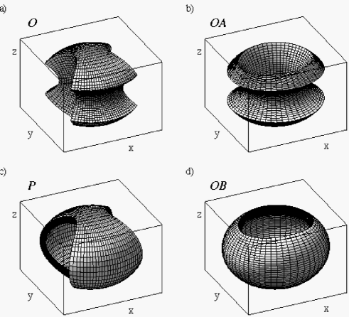
Figure 3: Caustics and boundary ellipsoid of the four types of invariant 3-tori for the ellipsoid with constants of the motion a) $(s_{1}^{2},s_{2}^{2})=(0.05,0.4)$, b) $(s_{1}^{2},s_{2}^{2})=(0.25,0.4)$, c) $(s_{1}^{2},s_{2}^{2})=(0.05,0.8)$, d) $(s_{1}^{2},s_{2}^{2})=(0.25,0.8)$.

The description of the free motion inside the ellipsoid in terms of the phase space variables $(\xi,\eta,\zeta,p_{\xi},p_{\eta},p_{\zeta})$ is rather complicated because of the change of coordinate sheets each time a boundary of the intervals in Eq. (9) is reached. Upon crossing one of the Cartesian coordinate planes $(x,y)$ or $(x,z)$ one of the momenta $p_{\xi}$, $p_{\eta}$ or $p_{\zeta}$ changes from $\pm\infty$ to $\mp\infty$, see Eq. (14) and Fig. 1. The singularities in Eq. (14) can be removed by a canonical transformation. The new coordinates are better suited for the semiclassical considerations in Section 5.

For the generating function of this canonical transformation we choose the ansatz

$$F_{2}=\lambda(\xi)p_{\lambda}+\mu(\eta)p_{\mu}+\nu(\zeta)p_{\nu}.$$ (17)

The index 2 indicates that this is a generating function of type 2 in the notation of H. Goldstein, see [26]. Then

$$\lambda=\frac{\partial F_{2}}{\partial p_{\lambda}},\,\,\mu=\frac{\partial F_{2}}{\partial p_{\mu}},\,\,\nu=\frac{\partial F_{2}}{\partial p_{\nu}}$$ (18)

are the new coordinates with $(p_{\lambda},p_{\mu},p_{\nu})$ the conjugate momentum variables. The transformation is completed by relating the old and new momentum variables:

$$p_{\xi}=\frac{d\lambda}{d\xi}p_{\lambda},\,\,p_{\eta}=\frac{d\mu}{d\eta}p_{\mu},\,\,p_{\zeta}=\frac{d\nu}{d\zeta}p_{\nu}.$$ (19)

To remove the singularities in Eq. (14) we require the above derivatives to be

$$\frac{d\lambda}{d\xi} = \quad\frac{a}{\sqrt{(\xi^{2}-a^{2})(\xi^{2}-b^{2})}},$$ (20)

$$\frac{d\mu}{d\eta} = -\frac{a}{\sqrt{(a^{2}-\eta^{2})(\eta^{2}-b^{2})}},$$ (21)

$$\frac{d\nu}{d\zeta} = \quad\frac{a}{\sqrt{(a^{2}-\zeta^{2})(b^{2}-\zeta^{2})}}.$$ (22)

Note the negative sign of the derivative $d\mu/d\eta$. These equations involve square roots of fourth order polynomials, i.e. they lead to elliptic integrals. Their inversion leads to elliptic functions. One finds

$$\xi(\lambda) = a\frac{{\,\mbox{dn}}(\lambda,q)}{{\,\mbox{cn}}(\lambda,q)},$$ (23)

$$\eta(\mu) = a{\,\mbox{dn}}(\mu,q^{\prime}),$$ (24)

$$\zeta(\nu) = b{\,\mbox{sn}}(\nu,q),$$ (25)

where ${\,\mbox{sn}}(\phi,q)$, ${\,\mbox{cn}}(\phi,q)$ and ${\,\mbox{dn}}(\phi,q)$ are Jacobi’s elliptic functions with ’angle’ $\phi$ and modulus $q$ [27]. Here the modulus is given by $q=b/a$. $q^{\prime}=(1-q^{2})^{1/2}$ denotes the conjugate modulus. This is the standard parameterization of the elliptic coordinates by elliptic functions, see e.g. [28]. For the momenta one finds

$$p_{\hat{s}}^{2}=\sigma_{\hat{s}}\frac{2E}{a^{2}}\left(s^{4}(\hat{s})-2ks^{2}(\hat{s})+l\right),$$ (26)

with $\hat{s}\in\{\lambda,\mu,\nu\}$ and $s(\hat{s})\in\{\xi(\lambda),\eta(\mu),\zeta(\nu)\}$ from Equations (23)-(25). The coefficients $\sigma_{\hat{s}}$ are the signs $\sigma_{\lambda}=\sigma_{\nu}=+$ and $\sigma_{\mu}=-$.

Transforming the coordinate ranges in Eq. (9) for the old coordinates $(\xi,\eta,\zeta)$ to the new coordinates gives

$$0\leq \lambda \leq{\cal F}\left(\chi,q\right),$$ (27)

$$0\leq \mu \leq{\cal K}(q^{\prime})={\cal K}^{\prime}(q),$$ (28)

$$0\leq \nu \leq{\cal K}(q),$$ (29)

for the motion in one octant. Here ${\cal F}(\chi,q)$ denotes Legendre’s incomplete elliptic integral of first kind with amplitude $\chi$ and modulus $q$ [27, 29]. The amplitude is given by

$$\sin^{2}\chi=\frac{1-a^{2}}{1-b^{2}}\,.$$ (30)

${\cal K}(q)$ is the complete elliptic integral of first kind with modulus $q$ and ${\cal K}^{\prime}(q)={\cal K}(q^{\prime})$ its complement. In the following we will omit the modulus in the notation for elliptic integrals because the modulus will not change in the course of this paper. The appearance of the incomplete integral is due to the fact that we cut off the coordinate range in the ellipsoidal direction, i.e. to the billiard character of the underlying motion. In terms of the Cartesian coordinates the coordinate ranges in Equations (27)-(29) yield the octant $x,y,z\geq 0$ within the ellipsoid. Inserting $(\lambda,\mu,\nu)$ into the expressions for the Cartesian coordinates in Eq. (8) gives

$$x = a\frac{{\,\mbox{dn}}(\lambda,q){\,\mbox{dn}}(\mu,q^{\prime}){\,\mbox{sn}}(\nu,q)}{{\,\mbox{cn}}(\lambda,q)},$$ (31)

$$y = q^{\prime}a\frac{{\,\mbox{cn}}(\mu,q^{\prime}){\,\mbox{cn}}(\nu,q)}{{\,\mbox{cn}}(\lambda,q)},$$ (32)

$$z = q^{\prime}a\frac{{\,\mbox{sn}}(\lambda,q){\,\mbox{sn}}(\mu,q^{\prime}){\,\mbox{dn}}(\nu,q)}{{\,\mbox{cn}}(\lambda,q)}.$$ (33)

The functions ${\,\mbox{sn}}(\phi)$ and ${\,\mbox{cn}}(\phi)$ both have period $4{\cal K}$ on the real axis, ${\,\mbox{dn}}(\phi)$ has period $2{\cal K}$. Extending the ranges in Equations (28) and (29) to the full real axis for $\mu$ and $\nu$ thus gives $x$, $y$ and $z$ as periodic functions of $\mu$ and $\nu$. If in addition to that we let $\lambda$ vary in the interval $[-{\cal F}(\chi),{\cal F}(\chi)]$ the billiard dynamics becomes smooth across the planes $(x,y)$, $(x,z)$ and $(y,z)$. We thus have a coordinate system that both separates Hamilton’s equations and the reflection condition and yields smooth dynamics inside the ellipsoid. The motion is thus best described as a geodesic flow on the product of an interval and a $2$-torus,

$$(\lambda,\mu,\nu)\in[-{\cal F}(\chi),{\cal F}(\chi)]\times T^{2},$$ (34)

i.e. on a solid 2-torus as depicted in Fig. 4. The flow is smooth except for the reflections at the boundaries $\lambda=\pm{\cal F}(\chi)$ which are still desribed by the sign change

$$(\lambda,\mu,\nu,p_{\lambda},p_{\mu},p_{\nu})\rightarrow(\lambda,\mu,\nu,-p_{\lambda},p_{\mu},p_{\nu}).$$ (35)

The whole torus

$$-{\cal F}\left(\chi\right)\leq \lambda \leq{\cal F}\left(\chi\right)\,,$$ (36)

$$0\leq \mu \leq 4{\cal K}^{\prime}\,,$$ (37)

$$0\leq \nu \leq 4{\cal K}$$ (38)

gives a fourfold cover of the interior of the ellipsoid.

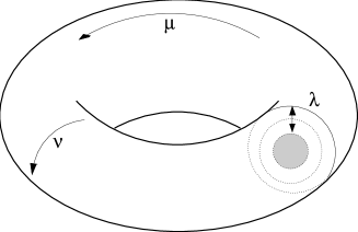
Figure 4: Solid $2$-torus as the fourfold cover of the configuration space of the billiard inside the ellipsoid.

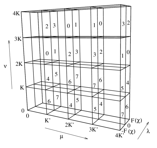
Figure 5: Representation of the solid $2$-torus (Fig. 4) of the configuration space as a cube with periodic boundaries in the directions of $\mu$ and $\nu$. Each small cube represents one $(x,y,z)$-octant. They are labeled in a ’binary’ way with respect to the signs of $x$,$y$ and $z$, i.e. $(-,-,-)$ corresponds to $0$, $(-,-,+)$ corresponds to 1, …, $(+,+,+)$ corresponds to $7$. The labels are put on the right side of each cube.

In Fig. 5 we represent the solid torus as a cube and mark the boundaries between the preimages of the different $(x,y,z)$-octants. Each $(x,y,z)$-octant gives a small cube

$$[0,\pm{\cal F}(\chi)]\times[n_{\mu}{\cal K}^{\prime},(n_{\mu}+1){\cal K}^{\prime}]\times[n_{\nu}{\cal K},(n_{\nu}+1){\cal K}]$$ (39)

with $(n_{\mu},n_{\nu})\in{\mathbb{Z}}^{2}$. The fact that each of the small cubes has to be bounded by 5 neighbouring small cubes to make the dynamics smooth can be understood in terms of the old variables $\xi$, $\eta$ and $\zeta$. Each $(x,y,z)$-octant is bounded by five singular sheets of the coordinates $(\xi,\eta,\zeta)$, see Fig. 1. Note that instead of considering the three real Equations (23)-(25) it is equivalent to consider only the $\zeta$ equation but for complex $\nu$ in the fundamental domain and use the idendities ${\,\mbox{sn}}(u+{\cal K}+i{\cal K}^{\prime},q)=q^{-1}{\,\mbox{dn}}(u,q)/{\,\mbox{cn}}(u,q)$ and ${\,\mbox{sn}}(-iu+{\cal K}+i{\cal K}^{\prime},q)=q^{-1}{\,\mbox{dn}}(u,q^{\prime})$.

The four covers of the ellipsoid are related by the group of involutions which leave the Cartesian coordinates in Equations (31)-(33) fixed. This group has three non-trivial elements

$$S_{1}(\lambda,\mu,\nu) = (-\lambda,-\mu,\nu)\,,$$ (40)

$$S_{2}(\lambda,\mu,\nu) = (\lambda,-\mu-2{\cal K}^{\prime},2{\cal K}-\nu)\,,$$ (41)

$$S_{3}(\lambda,\mu,\nu) = (-\lambda,\mu-2{\cal K}^{\prime},2{\cal K}-\nu)\,.$$ (42)

Any two of them generate the group which is isomorphic to the dihedral group $D_{2}$ (also called “Kleinsche Vierergruppe” [30]).

Inspection of Equations (31)-(33) shows that it is justifiable to think of $\mu$ as a kind of rotational angle about the $x$-axis. In the $y$-component and $z$-component $\mu$ appears as the argument of the elliptic functions sn and cn which are similar to the trigonometric functions sine and cosine. Similarly $\nu$ can be considered as a rotation angle about the $z$-axis. The types of motion in Fig. 3 therefore have the interpretations of $\mu$-rotations for type $P$ and $\nu$-rotations with different $\mu$-oscillations for types $OA$ and $OB$.

In Fig. 5 each column

$$[-{\cal F}(\chi),{\cal F}(\chi)]\times[n_{\mu}{\cal K}^{\prime},(n_{\mu}+1){\cal K}^{\prime}]\times[0,4{\cal K}]$$ (43)

with $n_{\mu}\in{\mathbb{Z}}$ fixed gives a single cover of the interior of the ellipsoid. This does not hold analogously for $\nu$. This is familiar from the polar coordinates of the sphere where $\nu$ should be compared to the azimutal angle and $\mu$ is similar to the polar angle.

For the semiclassical quantization in Section 5 it is helpful to deal with a simple kinetic-plus-potential-energy Hamiltionian. We therefore write Eq. (26) in the form

$$E_{\hat{s}}=\frac{p_{\hat{s}}^{2}}{2}+V_{\hat{s}}(\hat{s})$$ (44)

with

$$E_{\hat{s}}=\sigma_{\hat{s}}\frac{E}{a^{2}}l$$ (45)

and

$$V_{\hat{s}}(\hat{s})=-\sigma_{\hat{s}}\frac{E}{a^{2}}(s^{4}(\hat{s})-2ks^{2}(\hat{s}))\,.$$ (46)

The effective potentials $V_{\mu}$ and $V_{\nu}$ are periodic functions with periods $2{\cal K}^{\prime}$ and $2{\cal K}$, respectively. $V_{\lambda}$ is symmetric about 0. The number of potential wells per period changes across the lines $2k=s_{1}^{2}+s_{2}^{2}=2a^{2}$ and $2k=s_{1}^{2}+s_{2}^{2}=2b^{2}$ indicated as the dashed lines $c_{\lambda}$ and $c_{\nu}$ in Fig. 2. Between $c_{\lambda}$ and $c_{\nu}$, $V_{\mu}$ has two maxima per period at integer multiples of ${\cal K}^{\prime}$, $V_{\nu}$ has one maximum per period at odd integer multiples of ${\cal K}$ and $V_{\lambda}$ has a single maximum at $\lambda=0$. The effective potentials and energies for this region in Fig. 2 are shown in Fig. 6. Above $c_{\lambda}$, $V_{\lambda}$ has a minimum at $\lambda=0$ and two symmetric maxima, and $V_{\mu}$ has only one maximum per period at odd integer multiples of ${\cal K}^{\prime}$. It is easy to check that the effective energy $E_{\lambda}$ is always less than the potential energy at the minimum at $\lambda=0$. This minimum thus has no consequences for the classical dynamics. At $c_{\lambda}$ in Fig. 2, $V_{\lambda}$ changes from one to two maxima, and at $P_{\lambda}$ we additionally have $V_{\lambda}(0)=E_{\lambda}$. $E_{\mu}$ reaches its minimum value relative to $V_{\mu}$ here. Below the line $c_{\nu}$ the maxima of $V_{\nu}$ at odd integer multiples of ${\cal K}$ change into local minima and $V_{\nu}$ has two maxima per period. The maxima of $V_{\mu}$ at odd integer multiples of ${\cal K}^{\prime}$ have vanished here and $V_{\mu}$ has one maximum per period. Again it is easy to check that the effective energy $E_{\nu}$ is always less then local minima of $V_{\nu}$ at odd integer multiples of ${\cal K}$. The local minima thus do not influence the classical dynamics. At $c_{\nu}$ in Fig. 2, $V_{\nu}$ changes from one to two minima and at $P_{\nu}$ we additionally have $V_{\nu}((2n+1){\cal K})=E_{\nu}$ for $n\in{\mathbb{Z}}$. $E_{\mu}$ reaches its minimum value relative to $V_{\mu}$ here. These cases are summarized in Fig. 7.

Figure 6: Effective potentials $V_{\hat{s}}$ (solid) together with the effective energies $E_{\hat{s}}$ (dotted) for the parts of the regions $O$, $OA$, $P$  and $OB$  with $2b^{2}\leq s_{1}^{2}+s_{2}^{2}\leq 2a^{2}$. At the top the reflections are indicated which determine the symmetry of the wave functions according to the parity at the reflection point, see Section 4.

Figure 7: Analogue of Fig. 6 for parameter combinations in Fig. 2 above the line $c_{\lambda}$ (first row), at $P_{\lambda}$ (second row), below the line $c_{\nu}$ (third row) and at $P_{\nu}$ (last row).

3 The Action Integrals

For the calculation of actions it is useful to inspect the caustics in Fig. 3. The action integrals are written in the form

$$I_{\hat{s}}\equiv I_{s}=\frac{1}{2\pi}\oint p_{s}\,ds=\frac{m_{s}}{2\pi}\int_{s_{-}}^{s_{+}}p_{s}\,ds$$ (47)

with $(\hat{s},s)\in\{(\lambda,\xi),(\mu,\eta),(\nu,\zeta)\}$. The integers $m_{s}$ and the integration boundaries $s_{-}$ and $s_{+}$ can be found in Tab. I, see [8], also the final comments in Section 2.

type	$m_{\xi}$	$m_{\eta}$	$m_{\zeta}$	$\xi_{-}$	$\xi_{+}$	$\eta_{-}$	$\eta_{+}$	$\zeta_{-}$	$\zeta_{+}$
$O$	$4$	$4$	$4$	$a$	$1$	$b$	$s_{2}$	$0$	$s_{1}$
$OA$	$4$	$2$	$\pm 4$	$a$	$1$	$s_{1}$	$s_{2}$	$0$	$b$
$P$	$2$	$\pm 4$	$4$	$s_{2}$	$1$	$b$	$a$	$0$	$s_{1}$
$OB$	$2$	$4$	$\pm 4$	$s_{2}$	$1$	$s_{1}$	$a$	$0$	$b$

Table I: Integration boundaries $s_{-}$ and $s_{+}$ and multipliers $m_{s}$ in Eq. (47) for the four types of motion $O$, $OA$, $P$ and $OB$.

For the symmetry reduced ellipsoidal billiard any motion is of oscillatory type always giving $m_{s}=2$. To distinguish the symmetry reduced actions from the actions of the full ellipsoid we write the former with tildes, i.e.

$$\tilde{I}_{\hat{s}}\equiv\tilde{I}_{s}=\frac{1}{\pi}\int_{s_{-}}^{s_{+}}p_{s}\,ds.$$ (48)

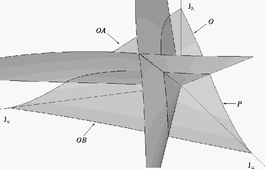
Figure 8: Energy surface and separatrix surfaces in the space of the actions $J$.

The presentation of the energy surface $H({\mbox{\boldmath$I$\unboldmath}})=E$ in the space of the actions $I$ is not smooth because an action variable can change discontinuously upon traversing a separatrix. In contrast to that the symmetry reduced system $\tilde{H}({\mbox{\boldmath$\tilde{I}$\unboldmath}})$ is continuous. For the quantum mechanical considerations it is advantagous to have a continuous energy surface even for the full system. We therefore introduce the actions

$${\mbox{\boldmath$J$\unboldmath}}=2{\mbox{\boldmath$\tilde{I}$\unboldmath}},$$ (49)

which have the property that the phase space volume below the energy surface $\tilde{H}({\mbox{\boldmath$J$\unboldmath}}/2)=E$ in the space of the actions $J$ is equal to the phase space volume below the energy surface $H({\mbox{\boldmath$I$\unboldmath}})=E$ in the space of the actions $I$ for the same energy $E$. In Fig. 8 $\tilde{H}({\mbox{\boldmath$J$\unboldmath}}/2)=E$ is shown together with the separatrix surfaces $s_{1}^{2}=b^{2}$ and $s_{2}^{2}=a^{2}$. Because the action variables scale with the energy the separatrix surfaces are foliated by rays through the origin. They divide the action space into the four regions corresponding to the different types of motion $O$, $P$, $OA$ and $OB$.

Figure 9: Riemann sphere $\overline{{\mathbb{C}}}$ with the critical points $z_{1},...,z_{6}$. The rectangular boundary with the point $z_{6}$ should be considered as the point $\infty$. The dashed line marks the boundary ellipsoid extented to the complex plane. The points $-i$ and $i$ are marked for reasons of orientation.

Figure 10: The glueing of 2 slit Riemann spheres to give the hyperelliptic curve ${\cal R}_{w}$. The horizontal plane marks the billiard boundary extended to $\overline{C}^{2}$. The points $-i$ and $i$ are marked for reasons of orientation.

Inserting the momenta from Eq. (26) and substituting $z=s^{2}$ in Eq. (47) shows that the action integrals are of the form

$$\int_{z_{-}}^{z_{+}}(z-s_{2}^{2})(z-s_{1}^{2})\,\frac{dz}{w}$$ (50)

with

$$w^{2}=\prod_{i=1}^{5}(z-z_{i})$$ (51)

where $z_{-}$, $z_{+}$ are sucessive members of $\{z_{1},z_{2},z_{3},z_{4},z_{5},z_{b}\}=\{0,s_{1}^{2},b^{2},s_{2}^{2},a^{2},1\}$. $z_{b}=1$ corresponds to the boundary of the billiard. The differential $dz/w$ has the six critical points $z_{1},...,z_{5}$ and $z_{6}=\infty$ which implies that the integrals in Eq. (50) are hyperelliptic. There do not exist tabulated standard forms for these integrals but there is the well developed theory of so called Abelian integrals. The main object of this theory is a Riemann surface, in our case the hyperelliptic curve

$${\cal R}_{w}=\{(z,w)\in\overline{{\mathbb{C}}}^{2}:w^{2}=\prod_{i=1}^{5}(z-z_{i})\}.$$ (52)

Here $\overline{{\mathbb{C}}}$ denotes the compactified complex plane, i.e. the Riemann sphere. To construct a picture of ${\cal R}_{w}$ we proceed in the following manner. We order the critical points $z_{i}$, $i=1,...,5$, according to their magnitudes. This gives $4$ orderings, one for each type of motion, e.g. $z_{1}=0$, $z_{2}=s_{1}^{2}$, $z_{3}=b^{2}$, $z_{4}=s_{2}^{2}$, and $z_{5}=a^{2}$ for type $O$, see Tab. I. The points $z_{i}$ are marked on the Riemann sphere, see Fig. 9. We then slit the Riemann sphere along the real axis between the points $z_{i}$ and $z_{i+1}$ for $i=1,3,5$. Excluding the three slits from $\overline{{\mathbb{C}}}$ the sign of $w$ is everywhere well defined on this manifold when it is fixed at one arbitrary point. In Fig. 9 we choose the sign of $w$ to be positive right above the slit $[z_{1},z_{2}]$. Then the sign is negative right above the slit $[z_{3},z_{4}]$ and again positive right above the slit $[z_{5},z_{6}]$. Right below the slits the sign of $w$ is opposite to the sign right above. Around the slits we have the closed paths $z_{1}\rightleftharpoons z_{2}$, $z_{3}\rightleftharpoons z_{4}$ and $z_{5}\rightleftharpoons z_{6}$. On another copy of $\overline{{\mathbb{C}}}$ we introduce the same slits but choose the sign of $w$ opposite to the choice on the former copy. The path from $z_{2}$ to $z_{3}$ on the former copy in Fig. 9 is assumed to be the first half of a closed path $z_{2}\rightleftharpoons z_{3}$ of which the second half from $z_{3}$ back to $z_{2}$ lies on the latter copy. The same is assumed to hold for the closed path $z_{4}\rightleftharpoons z_{5}$. To unify the view glue the two copies at the corresponding slits such that the corresponding critical points coincide and such that $w$ changes smoothly across the seams, see Fig. 10. The result is a compact Riemann surface, i.e. a manifold which carries a complex structure and to which the full machinery of Cauchy integration theory is applicable. The surface has genus $g=2$ and there are 4 non-contractable paths on the manifold which cannot be transformed smoothly into each other. They form a basis of the four-dimensional homology group corresponding to this surface. The homology basis may be specified by the choice of the closed paths $z_{1}\rightleftharpoons z_{2}$, $z_{2}\rightleftharpoons z_{3}$, $z_{3}\rightleftharpoons z_{4}$ and $z_{4}\rightleftharpoons z_{5}$. The path $z_{5}\rightleftharpoons z_{6}$ is homologous to the sum of $z_{1}\rightleftharpoons z_{2}$ and $z_{3}\rightleftharpoons z_{4}$ then. From the non-trivial topology of the Riemann surface ${\cal R}_{w}$ it follows that there may exist non-vanishing closed integrals (even for vanishing residues). The action integral Eq. (50) is of this type. It is an integral with singularities but vanishing residues - a so called Abelian integral of second kind. The actions integrals $I_{\nu}$ and $I_{\mu}$ of Eq. (50) are taken along the closed paths $z_{1}\rightleftharpoons z_{2}$ and $z_{3}\rightleftharpoons z_{4}$. Due to the reflection at the boundary ellipsoid the action integral $I_{\lambda}$ is not taken along a closed path. It is taken along the slit $[z_{5},z_{6}]$, but only between $z_{5}$ and $z_{b}$. It is therefore called incomplete. The integrals $I_{\mu}$ and $I_{\nu}$ are called complete. These three integrals give real numbers. In contrast to this the integration of Eq. (50) along the closed paths $z_{2}\rightleftharpoons z_{3}$ and $z_{4}\rightleftharpoons z_{5}$ yields purely imaginary numbers. These integrals have an important physical meaning for the semiclassical quantization scheme in Section 5. They give the penetration integrals which will be needed for the discussion of quantum mechanical tunneling. At this stage we already mention that there are only two such penetration integrals and we define them as follows:

$$\Theta_{\nu} \equiv \Theta_{\zeta}=-2i\int_{s_{1}}^{b}p_{\zeta}\,d\zeta,$$ (53)

$$\Theta_{\lambda} \equiv \Theta_{\xi}=-2i\int_{a}^{s_{2}}p_{\xi}\,d\xi.$$ (54)

The factor $i$ in the definition turns both integrals into real numbers. It is useful to take these definitions independent from the type of motion $O$, $OA$, $P$  and $OB$, i.e. for any ordering of $b$, $s_{1}$, $a$ and $s_{2}$. This will become clear in Section 5.

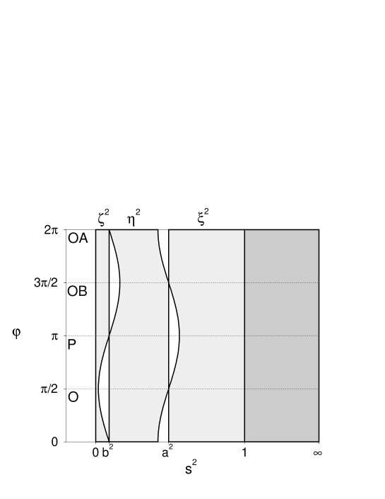
Figure 11: The parameter ranges for $s^{2}\in\{\zeta^{2},\eta^{2},\xi^{2}\}$ define a family of hyperelliptic curves parametrized by the angle $\varphi$ in Fig 2.

In Fig. 11 we show the ranges for the coordinates $s^{2}\in\{\zeta^{2},\eta^{2},\xi^{2}\}$ on the circle in the parameter plane in Fig. 2. Generically the ranges for $\zeta^{2}$ and $\eta^{2}$ and the ranges for $\eta^{2}$ and $\xi^{2}$ are separated by finite gaps. This gives the Riemann surfaces of genus 2 as described above. Now consider the circle in Fig. 2. On the bifurcation lines which are reached for angle $\varphi$ equal to integer multiples of $\pi/2$ one of the two gaps vanishes. One of the penetration integrals in Eq. (53) then vanishes too. This means that two of the three slits in Fig. 9 merge and the genus of the Riemann surface is diminished by one. On the bifurcation lines we thus find elliptic curves (genus 1) with an additional pole in the differential for the actions. They can also be considered as singular hyperelliptic curves. The three action integrals and the one remaining penetration integral are of elliptic type then. In [8] analytic expression in terms of Legendre’s standard integrals are calculated for these cases.

4 The Quantum System

The quantum mechanical billiard problem is the problem of determining the spectrum of the Laplacian in the billiard domain with Dirichlet boundary conditions on the boundary. Equivalently, this is given by Schrödinger’s equation for a free particle in the ellipsoid which in turn is Helmholtz’s equation in three dimensions,

$$-\frac{\hbar^{2}}{2}{\mbox{\boldmath$\nabla$\unboldmath}}^{2}\psi=E\psi.$$ (55)

As in the classical case the potential vanishes inside the ellipsoid and is infinite outside the ellipsoid. This potential classically leads to elastic reflections and quantum mechanically imposes Dirichlet boundary conditions on the ellipsoid. The three discrete symmetries of the ellipsoid are the reflections at the three Cartesian coordinate planes. The wave function can have even or odd parity with respect to each discrete symmetry, $\psi(x,y,z)=\pi_{x}\psi(-x,y,z)$ etc. Combining the two parities for each dimension we obtain a total of eight parity combinations denoted by ${\mbox{\boldmath$\pi$\unboldmath}}=(\pi_{x},\pi_{y},\pi_{z})$ where each parity is from $\{+,-\}$.

Corresponding to the two sets of classical coordinates we get two sets of quantum mechanical equations. In both cases the separation is the same as in the classical case and the wave function $\psi$ is a product of three separated wave functions. The ellipsoidal coordinates $(\xi,\eta,\zeta)$ lead to the analogue of Eq. (14), which is

$$-\hbar^{2}\left(\sqrt{(s^{2}-a^{2})(s^{2}-b^{2})}\frac{d}{ds}\right)^{2}\psi_{s}(s)=2E\left(s^{4}-2ks^{2}+l\right)\,\psi_{s}(s)$$ (56)

with $s\in\{\xi,\eta,\zeta\}$. If we set $E=0$ but keep $K$ and $L$ finite we obtain one of the many forms of the Lamé equation [28, 31]. Since we are not only interested in the solution of the Laplace equation in the ellipsoid but in the spectrum of the Laplacian we have to consider this generalized Lamé equation, known as the ellipsoidal wave equation.

Transforming the equation into the regularized coordinates leads to the analogue of Eq. (26),

$$-\hbar^{2}a^{2}\sigma_{\hat{s}}\frac{d^{2}}{d\hat{s}^{2}}\psi_{\hat{s}}(\hat{s})=2E\left(s(\hat{s})^{4}-2ks(\hat{s})^{2}+l\right)\,\psi_{\hat{s}}(\hat{s})$$ (57)

where $\hat{s}\in\{\lambda,\mu,\nu\}$ and $s(\hat{s})\in\{\xi(\lambda),\eta(\mu),\zeta(\nu)\}$ from Equations (23)-(25). Comparing to the equations for the billiard in the ellipse [32] Eq. (57) is analogous to the Mathieu equation(s) in its standard form, while Eq. (56) is analogous to its algebraic form. Note that similar to the classical case it would be sufficient to only consider the equation for $\nu$ in the complex domain instead of the three equations for real arguments.

The Dirichlet boundary conditions require that the wave function $\psi(\lambda,\mu,\nu)=\psi_{\lambda}(\lambda)\psi_{\mu}(\mu)\psi_{\nu}(\nu)$ is zero on the ellipsoid, which gives $\psi_{\lambda}(\pm{\cal F}(\chi))=0$. The solutions in the two angular variables $\mu$ and $\nu$ must be periodic with periods $4{\cal K}^{\prime}$ and $4{\cal K}$, respectively, in order to give a smooth function on the solid 2-torus described in Section 2.

For $\mu$ and $\nu$, Eq. (57) is a linear differential equation with periodic coefficients. Floquet theory guarantees the existence of solutions $\psi_{\mu}$ with period an integer multiple of $2{\cal K}^{\prime}$ and solutions $\psi_{\nu}$ with period an integer multiple of $2{\cal K}$, respectively. The involutions $S_{1}$, $S_{2}$ and $S_{3}$ in Equations (40)-(42) relate the symmetries of the separated wave functions to the parities $\pi_{x}$, $\pi_{y}$ and $\pi_{z}$. Starting with $S_{1}$ the separation of the invariance condition $\psi(\lambda,\mu,\nu)=\psi(S_{1}(\lambda,\mu,\nu))$ gives

$$\frac{\psi_{\lambda}(\lambda)}{\psi_{\lambda}(-\lambda)}=\frac{\psi_{\mu}(-\mu)}{\psi_{\mu}(\mu)}.$$ (58)

Since the left hand side and the right hand side are functions of $\lambda$ and $\mu$ alone they have to be equal to some common constant. Because we may change the sign of $\lambda$ and $\mu$ independently giving the reciprocals of both sides of Eq. (58) the separation constant must have unit modulus. From Eq. (33) we see that the sign is the parity $\pi_{z}$. Similarly, from the invariance of $\psi$ under $S_{2}$ we get

$$\frac{\psi_{\mu}(-\mu-2{\cal K}^{\prime})}{\psi_{\mu}(\mu)}=\frac{\psi_{\nu}(\nu)}{\psi_{\nu}(2{\cal K}-\nu)}\,.$$ (59)

From replacing $\mu$ by $-\mu-2{\cal K}^{\prime}$ and/or $\nu$ by $2{\cal K}-\nu$ we see that both sides of Eq. (59) again have to be equal to a separation constant of unit modulus. With the aid of Eq. (32) we may identify the sign with the parity $\pi_{y}$. $\pi_{y}$ thus gives the parity of the wave function $\psi_{\mu}$ for reflections about ${\cal K}^{\prime}$ and of $\psi_{\nu}$ for reflections about ${\cal K}$. From the invariance of $\psi$ with respect to $S_{3}$ we get

$$\frac{\psi_{\lambda}(-\lambda)}{\psi_{\lambda}(\lambda)}\frac{\psi_{\mu}(\mu-2{\cal K}^{\prime})}{\psi_{\mu}(\mu)}=\frac{\psi_{\nu}(\nu)}{\psi_{\nu}(2{\cal K}-\nu)}$$ (60)

or with the results from above

$$\psi_{\mu}(\mu-2{\cal K}^{\prime})=\pi_{y}\pi_{z}\psi_{\mu}(\mu)\,.$$ (61)

This relates the product of the parities $\pi_{y}$ and $\pi_{z}$ to the period of $\psi_{\mu}$. $\psi_{\mu}$ is $2{\cal K}^{\prime}$-periodic for $\pi_{y}\pi_{z}=+$ and $4{\cal K}^{\prime}$-periodic (i.e. not $2{\cal K}^{\prime}$-periodic) for $\pi_{y}\pi_{z}=-$. Similar arguments hold for the wave function $\psi_{\nu}$. Here $\pi_{x}$ gives the symmetry of $\psi_{\nu}$ for reflections about 0. The product of the parities $\pi_{x}$ and $\pi_{y}$ determines its period: $\psi_{\nu}$ is $2{\cal K}$-periodic for $\pi_{x}\pi_{y}=+$ and $4{\cal K}$-periodic (i.e. not $2{\cal K}$-periodic) for $\pi_{x}\pi_{y}=-$. The parities for the separated wave functions are shown at the top of Fig. 6.

Even though the ellipsoidal coordinates $(\xi,\eta,\zeta)$ are not regular, the parities are most simply expressed by properties of the wave functions in these singular coordinates. Let us first rewrite Eq. (56) in the form

$$f\psi^{\prime\prime}+g\psi^{\prime}+h\psi/\hbar^{2}=0$$ (62)

with the polynomials

$$f(s) = (s^{2}-a^{2})(s^{2}-b^{2}),$$ (63)

$$g(s) = f^{\prime}(s)/2=s(2s^{2}-a^{2}-b^{2}),$$ (64)

$$h(s) = 2E(s^{4}-2ks^{2}+l)\,.$$ (65)

The singularities of  Eq. (62) and equivalently of Eq. (56) are given by the zeroes $\pm a$ and $\pm b$ of $f$. We postpone the question of additional singularities at infinity to Section 6 because they are not important for our numerical calculations. In order to look at the asymptotics of the solutions of Eq. (62) at the singular points we calculate the corresponding indicial equations. Denoting the position of the singularity under consideration by $c$, the exponents $\alpha$ of the solutions are the solutions of the indicial equation (see e.g. [28])

$$\alpha^{2}+(p_{c}-1)\alpha+q_{c}=0,$$ (66)

where

$$p_{c}=\lim_{s\rightarrow c}\frac{g(s)}{f(s)}(s-c),\quad q_{c}=\lim_{s\rightarrow c}\frac{h(s)}{f(s)}(s-c)^{2}.$$ (67)

To calculate $p_{c}$ it is best to perform the partial fraction decomposition of $g/f$,

$$\frac{g(s)}{f(s)}=\frac{1}{2}\left(\frac{1}{s-b}+\frac{1}{s+b}+\frac{1}{s-a}+\frac{1}{s+a}\right).$$ (68)

From this it is obvious that $p_{c}=1/2$ for all singular points. Since $h/f$ only has simple poles $q_{c}=0$, the exponents are $0$ and $1/2$. Because the singularities of the wave equations do not produce essential singularities in its solutions these singularities are called regular. In our case the two exponents refer to the two parities possible at a regular singular point. We require $\psi_{\eta}(b)=\psi_{\zeta}(b)=0$ for $\pi_{y}=-$ and $\psi_{\eta}(b)=\psi_{\zeta}(b)=1$ (up to normalization) for $\pi_{y}=+$. Similarly the value at the regular singular point $a$ of the wave functions $\psi_{\xi}$ and $\psi_{\eta}$ determines the parity $\pi_{z}$. For $\pi_{x}$ it is a little simpler, because it is determined by the value of $\psi_{\zeta}$ at the ordinary point $\zeta=0$. The boundary condition at $\xi=1$ always is $\psi_{\xi}(1)=0$. The need for the solution to be invariant under an additional symmetry group (arising e.g. if we work on a covering space) does not appear, because we only solve the wave function in one octant. The boundary conditions are summarized in Tab. II. Note that in line with the above considerations the table shows a very simple structure: the sign $-$ or $+$ in the first three parity columns successively determine the value $0$ or $1$ of the wave functions at $0$, $b$ and $a$.

$\pi_{x}$	$\pi_{y}$	$\pi_{z}$	$\psi_{\zeta}(0)$	$\psi_{\zeta}(b)$	$\psi_{\eta}(b)$	$\psi_{\eta}(a)$	$\psi_{\xi}(a)$	$\psi_{\xi}(1)$	$\psi_{\nu}$ period	$\psi_{\mu}$ period	nodal planes
$-$	$-$	$-$	0	0	0	0	0	0	$2{\cal K}$	$2{\cal K}^{\prime}$	$(x,y)$, $(x,z)$, $(y,z)$
$-$	$-$	$+$	0	0	0	1	1	0	$2{\cal K}$	$4{\cal K}^{\prime}$	$(x,z)$, $(y,z)$
$-$	$+$	$-$	0	1	1	0	0	0	$4{\cal K}$	$4{\cal K}^{\prime}$	$(x,y)$, $(y,z)$
$-$	$+$	$+$	0	1	1	1	1	0	$4{\cal K}$	$2{\cal K}^{\prime}$	$(y,z)$
$+$	$-$	$-$	1	0	0	0	0	0	$4{\cal K}$	$2{\cal K}^{\prime}$	$(x,y)$, $(x,z)$
$+$	$-$	$+$	1	0	0	1	1	0	$4{\cal K}$	$4{\cal K}^{\prime}$	$(x,z)$
$+$	$+$	$-$	1	1	1	0	0	0	$2{\cal K}$	$4{\cal K}^{\prime}$	$(x,y)$
$+$	$+$	$+$	1	1	1	1	1	0	$2{\cal K}$	$2{\cal K}^{\prime}$	$-$

Table II: Parities, boundary conditions of the separated wave functions $\psi_{s}$, periods of the separated wave functions $\psi_{\nu}$ and $\psi_{\mu}$, and Cartesian nodal planes.

In our numerical procedure we are going to start integrating at the regular singular points. Since this is impossible for initial conditions belonging to the solution with exponent $\alpha=1/2$ we have to factor out this behaviour analytically. To find solutions with the parities $\pi_{z}=-$ and/or $\pi_{y}=-$ we employ the transformations

$$\pi_{y}=+,\pi_{z}=- : \psi=\sqrt{s^{2}-a^{2}}\tilde{\psi}_{+-},$$ (69)

$$\pi_{y}=-,\pi_{z}=+ : \psi=\sqrt{s^{2}-b^{2}}\tilde{\psi}_{-+},$$ (70)

$$\pi_{y}=-,\pi_{z}=- : \psi=\sqrt{s^{2}-a^{2}}\sqrt{s^{2}-b^{2}}\tilde{\psi}_{--},$$ (71)

and leave $\psi=\tilde{\psi}_{++}$ unchanged for $\pi_{y}=\pi_{z}=+$. The polynomials $h$ and $g$ in Eq. (62) change according to

$$\begin{array}[]{ll}\tilde{h}_{+-}(s)=h(s)+2s^{2}-b^{2},&\tilde{g}_{+-}(s)=g(s)+2s(s^{2}-b^{2}),\\ \tilde{h}_{-+}(s)=h(s)+2s^{2}-a^{2},&\tilde{g}_{-+}(s)=g(s)+2s(s^{2}-a^{2}),\\ \tilde{h}_{--}(s)=h(s)+6s^{2}-b^{2}-a^{2},&\tilde{g}_{--}(s)=g(s)+2s(2s^{2}-b^{2}-a^{2}).\end{array}$$ (75)

The functions $\tilde{h}_{++}=h$ and $\tilde{g}_{++}=g$ remain unchanged. The resulting transformed equations change the prefactor $1/2$ in Eq. (68) to $3/2$ for the terms involving $\pm a$, $\pm b$, or both, respectively. Hence $p_{c}=3/2$ at the correponding regular singular point and $\alpha=0,-1/2$. We are now able to start integrating at the singular points $c=a$ or $c=b$, or to be more precise, a distance $\Delta s$ away from them, always with the special velocity that corresponds to the regular solution with exponent $\alpha=0$. The initial conditions are

$$\tilde{\psi}^{\prime}(c\pm\Delta s)=-\frac{\tilde{h}(c)}{\tilde{g}(c)},\quad\tilde{\psi}(c\pm\Delta s)=1\pm\Delta s\,\tilde{\psi}^{\prime}(c\pm\Delta s).$$ (76)

In order to find $\tilde{\psi}$, three conditions on the three separated wave functions $\tilde{\psi}_{s}$ have to be fulfilled simultaneously. This is possible because there are three parameters $E$, $k$ and $l$ in the three equations. However, each equation depends on all the three separation constants; the equations are separated but the constants are not. We use a numerical procedure similar to that described in [32], the essential difference being that for the ellipsoid the wave function $\tilde{\psi}_{\eta}$ has a regular singular point on both ends of the interval. Since it is not possible to integrate a regular solution into a singular point, but only away from it, we divide the interval into two equal parts $[b,(a+b)/2]$ and $[(a+b)/2,a]$ and require the solution to match smoothly at $s=(a+b)/2$. This is called shooting to a fitting point [33]. These two and the two remaining intervals $[0,b]$ and $[a,1]$ are all transformed to $[0,1]$, and the resulting system of four equations is simultaneously solved. With Newton’s method [33] the three free parameters are adjusted to satisfy the three remaining conditions $\tilde{\psi}_{\xi}(1)=0$, the smoothness condition at the fitting point $(a+b)/2$ for $\tilde{\psi}_{\eta}$ and $\tilde{\psi}_{\zeta}^{\prime}(0)=0$ for $\pi_{x}=+$ or $\tilde{\psi}_{\zeta}(0)=0$ for $\pi_{x}=-$, respectively. Taking the semiclassical values for $E$, $k$ and $l$ from Section 5 as an initial guess, the method always converges to the exact eigenvalues.

Figure 12: The eight transformed eigenfunctions $\tilde{\psi}$ with all quantum numbers 1 and all possible parities, i.e. $|1,1,1;\pm\pm\pm\rangle$. The parity $\pi_{x}$ is $-$ for wave functions starting at 0 and $+$ otherwise. The remaining two parities $\pi_{y},\pi_{z}$ are distinguished by the dashing.

Because we are free in the normalization of the three separated wave functions $\tilde{\psi}_{s}$ they can be multiplied by constant factors to give one smooth function on the interval $[0,1]$, see Fig. 12. $\tilde{\psi}$ has $n$ zeroes $\in(0,b)$, $m$ zeroes $\in(b,a)$ and $r$ zeroes $\in(a,1)$. The quantum numbers $(r,m,n)$ together with the parities ${\mbox{\boldmath$\pi$\unboldmath}}=(\pi_{x},\pi_{y},\pi_{z})$ completely determine the state which we denote by $|r,m,n;\pi_{x}\pi_{y}\pi_{z}\rangle$. The quantum numbers $(r,m,n)$ belong to the reduced system in one octant; the parities determine the wave function on the boundaries of the octant. It is not so simple to count the corresponding number of nodal surfaces in the full system. It is complicated by the fact that the $(x,y)$-plane and $(x,z)$-plane are composed of two different types of quadrics, see Fig. 1. Away from the three Cartesian coordinate planes the number of ellipsoidal nodal surfaces is counted by $r$, the number of one sheeted hyperboloidal nodal surfaces (“rotating” about the shortest semiaxis $z$) is given by $m$ and the number of two sheeted hyperboloidal nodal surfaces (“rotating” about the longest semiaxis $x$) is given by $n$, but because each surface has two sheets this makes $2n$ nodal surfaces. Depending on the parity combinations $\pi$ the Cartesian coordinate planes give additional nodal planes according to the last column of Tab. II.

5 Semiclassical Quantization

The semiclassical quantization of the ellipsoidal billiard is obtained from single valuedness conditions that are imposed on WKB wave functions on the fourfold cover discussed in Section 2. Let us consider Schrödinger’s equation for a general one dimensional Hamiltonian of the form

$$\hat{H}=-\frac{\hbar^{2}}{2}\frac{\partial^{2}}{\partial q^{2}}+V(q)\,.$$ (77)

For a fixed energy $E$ in each region $j$ between two successive classical turning points a WKB wave function of the form

$$\psi^{(j)}(q)=\left(A_{+}^{(j)}\exp(iS_{j}(q)/\hbar)+A_{-}^{(j)}\exp(-iS_{j}(q)/\hbar)\right)/\sqrt{p(q)}$$ (78)

is reasonable. Its phase is given by

$$S_{j}(q)=\int_{q_{j}}^{q}p(q^{\prime})\,dq^{\prime}$$ (79)

with the classical momentum $p(q)=\sqrt{2(E-V(q))}$. $A_{+}^{(j)}$ and $A_{-}^{(j)}$ are constants. The reference point $q_{j}$ for the phase integral is an arbitrary point in the region under consideration but it is convenient to take it as the left or right classical turning point although the WKB wave function is a good approximation only away from the classical turning points.

In the following we will consider WKB wave functions only in classically allowed regions although they are valid even in regions where $E<V(q)$ giving real exponentials in Eq. (78). The amplitude vectors ${\mbox{\boldmath$A$\unboldmath}}^{(1)}=(A_{+}^{(1)},A_{-}^{(1)})^{t}$ and ${\mbox{\boldmath$A$\unboldmath}}^{(2)}=(A_{+}^{(2)},A_{-}^{(2)})^{t}$ of WKB wave functions in two classically allowed regions 1 and 2 separated by a classically forbidden region are related by the matrix equation ${\mbox{\boldmath$A$\unboldmath}}^{(2)}=M(\Theta){\mbox{\boldmath$A$\unboldmath}}^{(1)}$ with the tunnel matrix (see [34] and the references therein)

$$M(\Theta)=e^{\Theta/\hbar}\left(\begin{array}[]{cc}\sqrt{1+e^{-2\Theta/\hbar}}&-i\\ i&\sqrt{1+e^{-2\Theta/\hbar}}\\ \end{array}\right)\,,$$ (80)

where

$$\Theta=-i\int_{q_{1}}^{q_{2}}p(q)\,dq$$ (81)

is the penetration integral of the potential barrier. Here $q_{1}$ and $q_{2}$ are the turning points to the left and right of the barrier, i.e. $V(q)<E$ for $q<q_{1}$ and $q>q_{2}$ and $V(q)>E$ for $q_{1}<q<q_{2}$. The matrix (80) remains valid if we increase the energy $E$ above the barrier’s maximum. Then the classical turning points become complex ($q_{1}$ complex conjugate to $q_{2}$) giving a negative penetration integral in Eq. (81). For $-\Theta\gg\hbar$ the matrix $M(\Theta)$ becomes the identity matrix.

The amplitude vectors ${\mbox{\boldmath$A$\unboldmath}}^{(1)}$ and ${\mbox{\boldmath$A$\unboldmath}}^{(2)}$ of two WKB wave functions defined in the same classically allowed region but with different reference points for the phase integral are related by the phase shift ${\mbox{\boldmath$A$\unboldmath}}^{(2)}=P(\phi){\mbox{\boldmath$A$\unboldmath}}^{(1)}$ with the matrix

$$P(\phi)=\left(\begin{array}[]{cc}\exp(i\phi/\hbar)&0\\ 0&\exp(-i\phi/\hbar)\end{array}\right)\,,$$ (82)

where $\phi=\int_{q_{1}}^{q_{2}}p(q)\,dq$.

Figure 13: Effective potential $V_{\mu}$ (solid line) and effective energy $E_{\mu}$ (dashed line) for motion type $OA$. The turning points $\mu_{i}$ ($i=1,...,8$) define WKB wave functions $\psi_{\mu}^{(i)}$ whose amplitudes are connected by the matrices $P$, $M_{1}$ and $M_{2}$.

Let us now specify the Hamiltonian (77) for the ellipsoidal billiard by the consideration of the effective potentials and energies defined in Equations (44)-(46). To illustrate the semiclassical quantization scheme we concentrate on the $\mu$ degree of freedom and again present the effective potential $V_{\mu}$ and energy $E_{\mu}$ for motion type $OA$ in Fig. 13. In the range $[0,4{\cal K}^{\prime}]$ we have the eight turning points $\mu_{i}$ marked in the figure. Taking them as the reference points for the definition of WKB wave functions we get two wave functions in each of the four classically allowed regions. The amplitude vectors ${\mbox{\boldmath$A$\unboldmath}}^{(1)}$ and ${\mbox{\boldmath$A$\unboldmath}}^{(2)}$ are connected by the phase shift matrix (82) with $\phi=\int_{\mu_{1}}^{\mu_{2}}p_{\mu}\,d\mu$. From Tab. I and the negative sign in Eq. (21) it becomes clear that $\phi=-(\pi/2)J_{\mu}$ with $J_{\mu}$ the action defined in Eq. (49). The matrix

$$P=\left(\begin{array}[]{cc}\exp(-i(\pi/2)J_{\mu}/\hbar)&0\\ 0&\exp(i(\pi/2)J_{\mu}/\hbar)\end{array}\right)$$ (83)

then also relates the pairs of amplitude vectors ${\mbox{\boldmath$A$\unboldmath}}^{(3)}$ and ${\mbox{\boldmath$A$\unboldmath}}^{(4)}$, ${\mbox{\boldmath$A$\unboldmath}}^{(5)}$ and ${\mbox{\boldmath$A$\unboldmath}}^{(6)}$, ${\mbox{\boldmath$A$\unboldmath}}^{(7)}$ and ${\mbox{\boldmath$A$\unboldmath}}^{(8)}$, see Fig. 13.

The amplitude vectors ${\mbox{\boldmath$A$\unboldmath}}^{(2)}$ and ${\mbox{\boldmath$A$\unboldmath}}^{(3)}$ are related by the tunnel matrix (80) where the penetration integral $\Theta=-i\int_{\mu_{2}}^{\mu_{3}}p_{\mu}\,d\mu$ is the penetration integral $\Theta_{\nu}$ defined in Eq. (53) (again see Tab. I and keep in mind the negative sign in Eq. (21)). The integration boundaries in the definition of $\Theta_{\nu}$ were independent of the classical type of motion. Therefore the connection relation remains valid if the effective energy and potential change such that we classically have a different type of motion, especially for motion types $O$ and $P$ where the turning points $\mu_{2}$ and $\mu_{3}$ become complex, see Fig 6. We set

$$M_{1}=M(-\Theta_{\nu})\,.$$ (84)

The matrix $M_{1}$ also connects the amplitude vectors ${\mbox{\boldmath$A$\unboldmath}}^{(6)}$ and ${\mbox{\boldmath$A$\unboldmath}}^{(7)}$.

Similarly one finds that the pairs of amplitude vectors ${\mbox{\boldmath$A$\unboldmath}}^{(4)}$, ${\mbox{\boldmath$A$\unboldmath}}^{(5)}$ and ${\mbox{\boldmath$A$\unboldmath}}^{(8)}$, ${\mbox{\boldmath$A$\unboldmath}}^{(1)}$ are related by the tunnel matrix

$$M_{2}=M(-\Theta_{\lambda})$$ (85)

with $\Theta_{\lambda}$ from Eq. (54) where we have taken into account the $4{\cal K}^{\prime}$-periodicity of the wave function $\psi_{\mu}$.

Starting at $\mu_{1}$ the quantization of the $\mu$ degree of freedom now reduces to finding an effective energy $E_{\mu}$ and an effective potential $V_{\mu}$ for which there exists a non-zero amplitude ${\mbox{\boldmath$A$\unboldmath}}^{(1)}$ which is mapped onto itself upon one traversal through the interval $[0,4{\cal K}^{\prime}]$, see Fig. 13. This is equivalent to the quantization condition

$$\det((M_{2}PM_{1}P)^{2}-{\mbox{\boldmath$1$\unboldmath}})=0$$ (86)

with $1$ the identity matrix. Similar quantization conditions can be found in [35, 36, 37, 38]. Because of $\det M(\Theta)=\det P(\phi)=1$, Eq. (86) may be rewritten as

$$\text{tr}\,(M_{2}PM_{1}P)^{2}=2\,.$$ (87)

The eigenvalues of Eq. (86) include all parity combinations $\pi_{y}$ and $\pi_{z}$. To distinguish between the different parities more information is needed. The parities give the additional conditions

$${\mbox{\boldmath$A$\unboldmath}}^{(3)}=\pi_{y}\left(\begin{array}[]{cc}0&1\\ 1&0\end{array}\right){\mbox{\boldmath$A$\unboldmath}}^{(2)} {\mbox{\boldmath$A$\unboldmath}}^{(7)}=\pi_{y}\left(\begin{array}[]{cc}0&1\\ 1&0\end{array}\right){\mbox{\boldmath$A$\unboldmath}}^{(6)}\,,$$ , (92)

$${\mbox{\boldmath$A$\unboldmath}}^{(5)}=\pi_{z}\left(\begin{array}[]{cc}0&1\\ 1&0\end{array}\right){\mbox{\boldmath$A$\unboldmath}}^{(4)} {\mbox{\boldmath$A$\unboldmath}}^{(1)}=\pi_{z}\left(\begin{array}[]{cc}0&1\\ 1&0\end{array}\right){\mbox{\boldmath$A$\unboldmath}}^{(8)}\,.$$ , (97)

These conditions have to be solved consistently with the above tunnel relations. From the various possibilities to do this we choose the following. We map the amplitude vector ${\mbox{\boldmath$A$\unboldmath}}^{(1)}$ from a point $\mu\in(\mu_{1},\mu_{2})$ to the point $\mu+2{\cal K}^{\prime}\in(\mu_{5},\mu_{6})$. From Eq. (61) we know that this produces the sign $\pi_{y}\pi_{z}$. There are two possibilities to replace one of the tunnel matrices in this map by the corresponding condition in Equations (92) and (97). We thus get the equations

$$B{\mbox{\boldmath$A$\unboldmath}}^{(1)}=0\,,\quad C{\mbox{\boldmath$A$\unboldmath}}^{(1)}=0$$ (98)

with the matrices

$$B = \pi_{z}\left(\begin{array}[]{cc}0&1\\ 1&0\end{array}\right)PM_{1}P-\pi_{y}\pi_{z}{\mbox{\boldmath$1$\unboldmath}}\,,$$ (101)

$$C = M_{2}P\pi_{y}\left(\begin{array}[]{cc}0&1\\ 1&0\end{array}\right)P-\pi_{y}\pi_{z}{\mbox{\boldmath$1$\unboldmath}}\,.$$ (104)

Eq. (98) is the analogue of Eq. (86) for half the interval $[0,4{\cal K}^{\prime}]$. We are free in the normalization of the WKB wave function. Setting $A_{+}^{(1)}=1$ we find $A_{-}^{(1)}=-B_{11}/B_{12}$. If we insert this into the equation involving the matrix $C$ and decompose the resulting equations into their real and imaginary parts the remaining independent conditions are

$$\cos(\pi J_{\mu}/\hbar)=\frac{\pi_{z}\pi_{y}e^{(\Theta_{\lambda}+\Theta_{\nu})/\hbar}-1}{\sqrt{\left(1+e^{2\Theta_{\lambda}/\hbar}\right)\left(1+e^{2\Theta_{\nu}/\hbar}\right)}}$$ (105)

and

$$\sin(\pi J_{\mu}/\hbar)=\frac{\pi_{z}e^{\Theta_{\lambda}/\hbar}+\pi_{y}e^{\Theta_{\nu}/\hbar}}{\sqrt{\left(1+e^{2\Theta_{\lambda}/\hbar}\right)\left(1+e^{2\Theta_{\nu}/\hbar}\right)}}\,.$$ (106)

These equations have to be fulfilled simultaneously. They are not independent of each another, but the relation is simple: the second equation is fulfilled on every second solution of the first equation.

For the $\lambda$ and $\nu$ degree of freedom we have to comment on the additional potential barriers in Fig. 7 appearing below the line $c_{\nu}$ and above the line $c_{\lambda}$ of the bifurcation diagram in Fig. 2. As we have mentioned in Section 2 the effective energies always lie below the additional local potential minima. They only reach the local minima at the points $P_{\nu}$ and $P_{\lambda}$, respectively. The corresponding classical turning points are always complex and therefore these barriers would enter the quantization scheme almost always with large negative penetration integrals, i.e. with tunnel matrices close to the identity matrix. The only exceptions occur in the regions close to the points $P_{\nu}$ and $P_{\lambda}$ which lie at the border of the bifurcation diagram. Here the action $J_{\mu}$ goes to zero, i.e. the semiclassical approximation is expected to give poor results anyway. The additional barriers will therefore not be taken into account. The quantization conditions for $\lambda$ and $\nu$ are then exactly the same as in the case of the planar elliptic billiard discussed in [32]. We only state the results. For the $\lambda$ degree of freedom one finds the two conditions

$$\cos(\pi J_{\lambda}/\hbar)=\frac{-\pi_{z}}{\sqrt{1+e^{2\Theta_{\lambda}/\hbar}}}$$ (107)

and

$$\sin(\pi J_{\lambda}/\hbar)=\frac{-1}{\sqrt{1+e^{-2\Theta_{\lambda}/\hbar}}}$$ (108)

and for the $\nu$ degree of freedom the conditions

$$\cos(\pi J_{\nu}/\hbar)=\frac{\pi_{x}\pi_{y}}{\sqrt{1+e^{2\Theta_{\nu}/\hbar}}}$$ (109)

and

$$\sin(\pi J_{\nu}/\hbar)=\frac{\pi_{x}}{\sqrt{1+e^{-2\Theta_{\nu}/\hbar}}}.$$ (110)

The actions $J_{\lambda}$ and $J_{\nu}$ are again taken from Eq. (49) and the only penetration integrals that appear are those defined in Equations (53) and (54).

Eq.	type $O$: $-\Theta_{\lambda},\Theta_{\nu}\gg\hbar$			type $OA$: $-\Theta_{\lambda},-\Theta_{\nu}\gg\hbar$
(107)	$-\pi_{z}$		$I_{\lambda}=J_{\lambda}=(n_{\lambda}+\frac{4}{4})\hbar$	$-\pi_{z}$		$I_{\lambda}=J_{\lambda}=(n_{\lambda}+\frac{4}{4})\hbar$
(108)	$0$	$\bigg{\}}$	$n_{\lambda}=2r+(1-\pi_{z})/2$	$0$	$\bigg{\}}$	$n_{\lambda}=2r+(1-\pi_{z})/2$
(105)	$0$		$I_{\mu}=J_{\mu}=(n_{\mu}+\frac{1}{2})\hbar$	$-1$		$I_{\mu}=J_{\mu}/2=(n_{\mu}+\frac{1}{2})\hbar$
(106)	$\pi_{y}$	$\bigg{\}}$	$n_{\mu}=2m+(1-\pi_{y})/2$	$0$	$\bigg{\}}$	$n_{\mu}=m$
(109)	$0$		$I_{\nu}=J_{\nu}=(n_{\nu}+\frac{1}{2})\hbar$	$\pi_{x}\pi_{y}$		$I_{\nu}=\pm J_{\nu}=\pm n_{\nu}\hbar$
(110)	$\pi_{x}$	$\bigg{\}}$	$n_{\nu}=2n+(1-\pi_{x})/2$	$0$	$\bigg{\}}$	$n_{\nu}=2n+(2-\pi_{x}-\pi_{y})/2$
Eq.	type P: $\Theta_{\lambda},\Theta_{\nu}\gg\hbar$			type $OB$: $\Theta_{\lambda},-\Theta_{\nu}\gg\hbar$
(107)	$0$		$I_{\lambda}=J_{\lambda}/2=(n_{\lambda}+\frac{3}{4})\hbar$	$0$		$I_{\lambda}=J_{\lambda}/2=(n_{\lambda}+\frac{3}{4})\hbar$
(108)	$-1$	$\bigg{\}}$	$n_{\lambda}=r$	$-1$	$\bigg{\}}$	$n_{\lambda}=r$
(105)	$\pi_{y}\pi_{z}$		$I_{\mu}=\pm J_{\mu}=\pm n_{\mu}\hbar$	$0$		$I_{\mu}=J_{\mu}=(n_{\mu}+\frac{1}{2})\hbar$
(106)	$0$	$\bigg{\}}$	$n_{\mu}=2m+(1-\pi_{y}\pi_{z})/2$	$\pi_{z}$	$\bigg{\}}$	$n_{\mu}=2m+(1-\pi_{z})/2$
(109)	$0$		$I_{\nu}=J_{\nu}=(n_{\nu}+\frac{1}{2})\hbar$	$\pi_{x}\pi_{y}$		$I_{\nu}=\pm J_{\nu}=\pm n_{\nu}\hbar$
(110)	$\pi_{x}$	$\bigg{\}}$	$n_{\nu}=2n+(1-\pi_{x})/2$	$0$	$\bigg{\}}$	$n_{\nu}=2n+(2-\pi_{x}-\pi_{y})/2$

Table III: Limiting quantization conditions for the 4 types of classical motion. The left hand sides of the braces in each box gives the limiting value of the right hand side of the equation cited in the very first column. The non-negative integers $n_{\lambda}$, $n_{\mu}$ and $n_{\nu}$ are related to the quantum numbers $r$, $m$ and $n$ introduced in Section 4, see Tab. I.

We first inspect the quantization conditions in Equations (105)-(110) for the limiting cases $|\Theta_{\lambda}|,|\Theta_{\nu}|\gg\hbar$. The signs of the penetration integrals $\Theta_{\lambda}$ and $\Theta_{\nu}$ determine the type of classical motion. The limiting cases $|\Theta_{\lambda}|,|\Theta_{\nu}|\gg\hbar$ thus correspond to the four regions in classical action space far away from the separatrix surfaces in Fig. 8. From the limiting quantization conditions for the actions $J$ the quantization of the original action variables $I$ can be deduced from Tab. I. We summarize the results in Tab. III. The limiting quantization conditions for $I$ may be compared with the EBK quantization in Eq. (4). From the identification of the Maslov phases ${\mbox{\boldmath$\alpha$\unboldmath}}=(\alpha_{\lambda},\alpha_{\mu},\alpha_{\nu})$ in the equations in Tab. III we find

$${\mbox{\boldmath$\alpha$\unboldmath}}=(4,2,2)\mbox{ for type $O$},\quad{\mbox{\boldmath$\alpha$\unboldmath}}=(4,2,0)\mbox{ for type $OA$},$$ (111)

$${\mbox{\boldmath$\alpha$\unboldmath}}=(3,0,2)\mbox{ for type $P$},\quad{\mbox{\boldmath$\alpha$\unboldmath}}=(3,2,0)\mbox{ for type $OB$}.$$ (112)

The Maslov indices $\alpha_{\mu}$ and $\alpha_{\nu}$ are in agreement with the simple EBK rule stated in the introduction: For motion of type $O$  $\mu$ and $\nu$ oscillate, for motion of type $P$ the motion is rotational in $\mu$ and oscillatory in $\nu$, $OA$ and $OB$ are oscillatory in the $\mu$ degree of freedom and rotational in $\nu$, see Section 2. For the $\lambda$ degree of freedom we have to take into account the reflection at the boundary ellipsoid which wave mechanically leads to Dirichlet boundary condition. For motion types $O$ and $OA$ $\lambda$ oscillates with two reflections giving $\alpha_{\lambda}=4$. For motion types $P$ and $OB$ $\lambda$ oscillates between the boundary ellipsoid and the caustic giving $\alpha_{\lambda}=3$.

$O$       $OA$

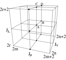
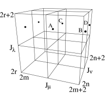
$P$       $OB$

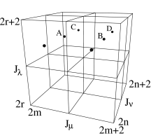
Figure 14: Quantum cells $\Delta J_{\lambda}=\Delta J_{\mu}=\Delta J_{\nu}=2$ in classical action space for the 4 limiting cases of classical types of motion. $J$ is measured in units of $\hbar$.

The EBK quantization condition in Eq. (4) defines a lattice in classical action space. The Maslov indices determine how this lattice is shifted relative to the simple lattice $({\mbox{\boldmath$n$\unboldmath}}\hbar)$. Since we have four different vectors of Maslov indices for the ellipsoidal billiard we have four different lattice types away from the separatrix surfaces in Fig. 8. We present the different lattices in Fig. 14 for quantum cells of width $\Delta J_{\lambda}=\Delta J_{\mu}=\Delta J_{\nu}=2\hbar$. Each cell contains eight quantum states. For motion type $O$  all states are non-degenerate. For motion types $OA$ and $OB$ each states is twofold quasidegenerate according to the two senses of rotation in $\nu$. Analogously for motion type $P$ each state is twofold quasidegenerate according to the two senses of rotation in the variable $\mu$. From the quantum mechanical point of view the quasidegeneracy can be understood in terms of the effective energies and potentials in Fig. 6. For eigenvalues which classically correspond to rotational motions far away from the classical separatrices the effective energy is much larger then the effective potential. The energy is then dominated by the kinetic energy, the specific shape of the potential becomes irrelevant. The effective energy then only depends on the net number of nodes of the wave function and not on the location of the nodes. Therefore wave functions with different symmetries but the same net number of nodes give the same effective energy. With the aid of Tab. III we can identify the states corresponding to the capital letters in Fig. 14, see Tab. IV.

$O$			$OA$
	A:	$|r,m,n;+++\rangle$		A:	$|r,m,n;+-+\rangle$,
	B:	$|r,m,n;+-+\rangle$			$|r,m,n;-++\rangle$
	C:	$|r,m,n;-++\rangle$		B:	$|r,m,n;--+\rangle$,
	D:	$|r,m,n;--+\rangle$			$|r,m,n+1;+++\rangle$
	E:	$|r,m,n;++-\rangle$		C:	$|r,m,n;+--\rangle$,
	F:	$|r,m,n;+--\rangle$			$|r,m,n;-+-\rangle$
	G:	$|r,m,n;-+-\rangle$		D:	$|r,m,n;---\rangle$,
	H:	$|r,m,n;---\rangle$			$|r,m,n+1;++-\rangle$
$P$			$OB$
	A:	$|r,m,n;++-\rangle$,		A:	$|r,m,n;+-+\rangle$,
		$|r,m,n;+-+\rangle$			$|r,m,n;-++\rangle$
	B:	$|r,m,n;+--\rangle$,		B:	$|r,m,n;+--\rangle$,
		$|r,m,n+1;+++\rangle$			$|r,m,n;-+-\rangle$
	C:	$|r,m,n;-+-\rangle$,		C:	$|r,m,n;--+\rangle$,
		$|r,m,n;--+\rangle$			$|r,m,n+1;+++\rangle$
	D:	$|r,m,n;---\rangle$,		D:	$|r,m,n;---\rangle$,
		$|r,m,n+1;-++\rangle$			$|r,m,n+1;++-\rangle$

Table IV: Quantum states in Fig. 14.

The quantization conditions in Equations (107)-(110) are uniform, i.e. they do not only give the limiting EBK lattices in Fig. 14 but also specify how these lattices join smoothly across the separatrix surfaces of Fig. 8. In the following we will refer to the uniform lattice in action space as WKB lattice. The transitions may be described in terms of effective Maslov phases. In order to see this we insert the EBK-like quantization conditions for the symmetry reduced ellipsoid

$${\mbox{\boldmath$\tilde{I}$\unboldmath}}={\mbox{\boldmath$J$\unboldmath}}/2=(\tilde{{\mbox{\boldmath$n$\unboldmath}}}+\tilde{{\mbox{\boldmath$\alpha$\unboldmath}}}/4)\hbar$$ (113)

with $\tilde{{\mbox{\boldmath$n$\unboldmath}}}=(r,m,n)$ into the left hand sides of Equations (107)-(110). The parities $\pi_{x}$, $\pi_{y}$ and $\pi_{z}$ on the right hand sides determine whether we have Dirichlet or Neumann boundary conditions on the corresponding piece of the Cartesian coordinate plane bounding the symmetry reduced ellipsoid. The different parity combinations altogether give the quantum states of the full ellipsoidal billiard. We now solve Equations (107)-(110) for the effective Maslov phases $\tilde{{\mbox{\boldmath$\alpha$\unboldmath}}}$. The quantum numbers $\tilde{{\mbox{\boldmath$n$\unboldmath}}}=(r,m,n)$ drop out because of the $2\pi$-periodicity of the trigonometric functions and it remains to invert the tangent on the correct branch which is determined by the parity combination. A little combinatorics gives

$$\tilde{\alpha}_{\lambda} = \pi_{z}\frac{2}{\pi}\arctan e^{\Theta_{\lambda}/\hbar}+3-\pi_{z},$$ (114)

$$\tilde{\alpha}_{\nu} = \pi_{y}\frac{2}{\pi}\arctan e^{\Theta_{\nu}/\hbar}+2-\pi_{x}-\pi_{y}.$$ (115)

For $\tilde{\alpha}_{\mu}$ this simple form cannot be achieved. Instead we write

$$\tilde{\alpha}_{\mu}=\frac{2}{\pi}\mbox{arg}\left(\pi_{z}\pi_{y}e^{(\Theta_{\lambda}+\Theta_{\nu})/\hbar}-1+i\left(\pi_{z}e^{\Theta_{\lambda}/\hbar}+\pi_{y}e^{\Theta_{\nu}/\hbar}\right)\right),$$ (116)

where arg maps the polar angle of a complex number to the interval $[0,2\pi)$. Essentially the effective Maslov phases consist of the simple switching function $(2/\pi)\arctan e^{x}$ which changes from 0 to 1 when $x$ changes from $-\infty$ to $+\infty$. From the simple form of the effective Maslov phases it follows that the ranges in which the semiclassically quantized action variables $J$ may vary are restricted according to ${\mbox{\boldmath$J$\unboldmath}}=(J_{\lambda},J_{\mu},J_{\nu})\mbox{ mod }2\hbar\in P_{\mbox{\boldmath$\pi$\unboldmath}}$, where the parity boxes $P_{\mbox{\boldmath$\pi$\unboldmath}}$ have side length $\hbar/2$ in the directions of $J_{\lambda}$ and $J_{\nu}$ and side length $\hbar$ in the direction $J_{\mu}$. For the different parity combinations $\pi$ we find

$$\begin{array}[]{lcccccc}P_{---}&=&[(3/2)\hbar,2\hbar]&\times&[\hbar,2\hbar]&\times&[(3/2)\hbar,2\hbar]\,,\\ P_{--+}&=&[\hbar,(3/2)\hbar]&\times&[(1/2)\hbar,(3/2)\hbar]&\times&[(3/2)\hbar,2\hbar]\,,\\ P_{-+-}&=&[(3/2)\hbar,2\hbar]&\times&[(1/2)\hbar,(3/2)\hbar]&\times&[\hbar,(3/2)\hbar]\,,\\ P_{-++}&=&[\hbar,(3/2)\hbar]&\times&[0,\hbar]&\times&[\hbar,(3/2)\hbar]\,,\\ P_{+--}&=&[(3/2)\hbar,2\hbar]&\times&[(\hbar,2\hbar]&\times&[(1/2)\hbar,\hbar]\,,\\ P_{+-+}&=&[\hbar,(3/2)\hbar]&\times&[(1/2)\hbar,(3/2)\hbar]&\times&[(1/2)\hbar,\hbar]\,,\\ P_{++-}&=&[(3/2)\hbar,2\hbar]&\times&[(1/2)\hbar,(3/2)\hbar]&\times&[0,(1/2)\hbar]\,,\\ P_{+++}&=&[\hbar,(3/2)\hbar]&\times&[0,\hbar]&\times&[0,(1/2)\hbar]\,,\end{array}$$ (117)

see Fig. 15.

Figure 15: The parity boxes $P_{{\mbox{\boldmath$\pi$\unboldmath}}}$ that contain the semiclassical states. $P_{-++}$ is obscured by the other parity boxes. $J$ is measured in units of $\hbar$.

Let us comment on the numerical procedure to solve the quantization condition (113). For given quantum numbers $\tilde{\mbox{\boldmath$n$\unboldmath}}$ and parity combination $\pi$ we have to find the corresponding zero of the function

$${\mbox{\boldmath$G$\unboldmath}}(E,s_{1}^{2},s_{2}^{2};{\mbox{\boldmath$\pi$\unboldmath}},\tilde{{\mbox{\boldmath$n$\unboldmath}}})={\mbox{\boldmath$\tilde{I}$\unboldmath}}(E,s_{1}^{2},s_{2}^{2})-(\tilde{{\mbox{\boldmath$n$\unboldmath}}}+\tilde{{\mbox{\boldmath$\alpha$\unboldmath}}}(E,s_{1}^{2},s_{2}^{2},{\mbox{\boldmath$\pi$\unboldmath}})/4)\hbar\,.$$ (118)

As in the exact quantum mechanical problem this problem is not separable for the separation constants and we have to apply Newton’s method in three dimensions. In order to find good starting values for Newton’s method we introduce an approximate function ${\mbox{\boldmath$G$\unboldmath}}_{\rm app}$ for $G$. The functional dependence of ${\mbox{\boldmath$G$\unboldmath}}_{\rm app}$, i.e. of the approximate actions ${\mbox{\boldmath$\tilde{I}$\unboldmath}}_{\rm app}$ and Maslov phases $\tilde{{\mbox{\boldmath$\alpha$\unboldmath}}}_{\rm app}$, on the parameters $(E,s_{1}^{2},s_{2}^{2})$ should be very simple such that the zeroes of ${\mbox{\boldmath$G$\unboldmath}}_{\rm app}$ can be found analytically. For $\tilde{{\mbox{\boldmath$\alpha$\unboldmath}}}_{\rm app}$ we simply take the mean value of $\tilde{\mbox{\boldmath$\alpha$\unboldmath}}$ for a given parity combination $\pi$. In order to get an expression for ${\mbox{\boldmath$\tilde{I}$\unboldmath}}_{\rm app}$ we take advantage of two properties of the energy surface in action space. Firstly the shape of the energy surface is very similar to a triangle and secondly up to a simple scaling the shape does not change with the energy. If we denote the intersections of the energy surface $E=1/2$ with the coordinate axes in action space by ${\bar{I}}_{\lambda}$, ${\bar{I}}_{\mu}$, and ${\bar{I}}_{\nu}$ the action variables can be approximated by

$${\mbox{\boldmath$\tilde{I}$\unboldmath}}_{\rm app}(E,s_{1}^{2},s_{2}^{2})=\sqrt{2E}\left[\left(\begin{array}[]{c}{\bar{I}}_{\lambda}\\ 0\\ 0\end{array}\right)+\gamma_{1}\left(\begin{array}[]{c}-{\bar{I}}_{\lambda}\\ 0\\ {\bar{I}}_{\nu}\end{array}\right)+\gamma_{2}\left(\begin{array}[]{c}-{\bar{I}}_{\lambda}\\ {\bar{I}}_{\mu}\\ 0\end{array}\right)\right]\ ,$$ (119)

where $\gamma_{1}$ and $\gamma_{2}$ parametrize the approximate triangular energy surface $E=1/2$. This can be considered as a crude periodic orbit quantization: we take the actions of the three stable isoltated periodic orbits of the system and approximate the whole energy surface by that of a harmonic oscillator that would have isolated stable orbits with those actions. The analogy has to be taken with care because our actions scale with $\sqrt{E}$, while those of the true harmonic oscillator are linear in the energy. The edges of this approximate energy surface are given by $\gamma_{1}=0$, $\gamma_{2}=0$, and $\gamma_{1}+\gamma_{2}=1$, respectively. In order to give $s_{1}$ and $s_{2}$ as functions of $\gamma_{1}$ and $\gamma_{2}$ it is useful to have a look at the asymptotic behavior of the actions and their approximations (119) upon approaching the edges of the energy surface. A simple calculation shows that $\tilde{I}_{\nu}$ behaves quadratically in $s_{1}$ for $s_{1}\to 0$. We set

$$s_{1}^{2}=a^{2}\gamma_{1}\,.$$ (120)

A similar consideration of the asymptotics of $\tilde{I}_{\lambda}$ for $s_{2}\to 1$ gives

$$s_{2}^{2}=1-(1-b^{2})(1-(\gamma_{1}+\gamma_{2}))^{2/3}\ .$$ (121)

In our numerical calculation the starting values obtained from these approximations always were sufficiently good to make Newton’s method converge to the right state. The quasidegeneracy of the states is no problem here because the degenerate states correspond to different parity combinations $\pi$. In Tab. V the semiclassical eigenvalues are compared to the exact quantum mechanical results. The semiclassical energy eigenvalues are always a little too low. The same is true for $k_{\rm sc}$ while $l_{\rm sc}$ tends to be too low. We do not have a good explanation for this.

$E_{{\text{qm}}}$	$k_{\text{qm}}$	$l_{\text{qm}}$	$E_{{\text{sc}}}$	$k_{\text{sc}}$	$l_{\text{sc}}$	$r$	$m$	$n$	$\pi_{x}$	$\pi_{y}$	$\pi_{z}$	$\Delta E$
6.65202	0.17113	0.01217	6.14810	0.20240	0.02052	0	0	0	$+$	$+$	$+$	7.6
12.1738	0.25651	0.04766	11.6003	0.27426	0.05007	0	0	0	$-$	$+$	$+$	4.7
12.5791	0.23997	0.02728	11.9202	0.26066	0.03416	0	0	0	$+$	$-$	$+$	5.2
16.0174	0.14696	0.00966	15.5690	0.15868	0.01338	0	0	0	$+$	$+$	$-$	2.8
19.3555	0.30548	0.07460	18.7075	0.31769	0.07694	0	0	1	$+$	$+$	$+$	3.3
19.4998	0.30161	0.06998	18.8698	0.31328	0.07198	0	0	0	$-$	$-$	$+$	3.2
21.2740	0.25695	0.01646	20.7491	0.26577	0.01936	0	1	0	$+$	$+$	$+$	2.5
23.4713	0.22232	0.03399	22.9153	0.23135	0.03520	0	0	0	$-$	$+$	$-$	2.4
23.9671	0.21138	0.01734	23.3068	0.22222	0.02081	0	0	0	$+$	$-$	$-$	2.8
⋮
1000.25	0.31235	0.08368	999.421	0.31266	0.08375	4	1	8	$+$	$+$	$-$	0.08
1000.25	0.31235	0.08368	999.421	0.31266	0.08375	4	1	7	$-$	$-$	$-$	0.08
1000.34	0.27684	0.04333	999.654	0.27705	0.04322	4	4	4	$+$	$-$	$-$	0.07
1001.11	0.43872	0.07161	998.606	0.43941	0.07165	0	10	5	$-$	$+$	$-$	0.25
1001.36	0.46428	0.19051	1000.49	0.46452	0.19067	1	2	12	$-$	$-$	$+$	0.09
1001.36	0.46428	0.19051	1000.49	0.46452	0.19067	1	2	13	$+$	$+$	$+$	0.09
1001.39	0.21559	0.01869	1000.78	0.21583	0.01876	6	4	1	$-$	$-$	$+$	0.06
1001.52	0.34082	0.09365	1001.38	0.34082	0.09365	3	2	8	$-$	$+$	$-$	0.01
1001.52	0.34082	0.09365	1001.38	0.34082	0.09365	3	2	8	$+$	$-$	$-$	0.01
1001.63	0.35433	0.03148	1000.62	0.35461	0.03156	1	11	2	$+$	$-$	$+$	0.10
1001.63	0.35433	0.03148	1000.62	0.35461	0.03156	1	11	2	$+$	$+$	$-$	0.10
1001.72	0.27396	0.03156	1000.31	0.27449	0.03168	4	6	2	$-$	$-$	$+$	0.14
1001.79	0.18851	0.02737	1001.45	0.18863	0.02732	7	1	3	$-$	$+$	$+$	0.03
1002.44	0.39897	0.00410	999.751	0.39971	0.00415	0	15	0	$+$	$-$	$+$	0.27
1002.44	0.39897	0.00410	999.751	0.39971	0.00415	0	15	0	$+$	$+$	$-$	0.27
1002.51	0.18815	0.02683	1002.23	0.18823	0.02672	7	1	3	$+$	$-$	$+$	0.03
1002.73	0.26921	0.00980	1002.49	0.26927	0.00986	3	9	0	$-$	$-$	$+$	0.02
1002.73	0.43764	0.06971	999.919	0.43852	0.07009	0	10	5	$+$	$-$	$-$	0.28
1002.95	0.39083	0.08511	1002.02	0.39107	0.08516	1	6	7	$-$	$+$	$-$	0.09
1002.95	0.39083	0.08511	1002.02	0.39107	0.08516	1	6	7	$+$	$-$	$-$	0.09

Table V: The quantum mechanical eigenvalues $(E_{{\text{qm}}},k_{\text{qm}},l_{\text{qm}})$ and the semiclassical eigenvalues $(E_{{\text{sc}}},k_{\text{sc}},l_{\text{sc}})$ of the ellipsoidal billiard for the ranges $E_{{\text{qm}}}<24$ and $1000<E_{{\text{qm}}}<1003$. The relative error $\Delta E=(E_{{\text{qm}}}-E_{{\text{sc}}})/E_{{\text{qm}}}$ is given in percent.

Let us first consider the four transitions of the WKB lattice in action space across the separatrix surfaces of Fig. 8 away from the intersection line of the separatrix surfaces. Upon each crossing only two effective Maslov phases change appreciably. We therefore take the action component of $J$ corresponding to the effective Maslov phase that stays approximately constant as being semiclassically quantized. To do so we have to fix the quantum number belonging to this action component and the parities appearing in its effective Maslov phase. The quantum numbers corresponding to the two other action components and the remaining free parities then define a family of surfaces in action space, which intersect the plane corresponding to the action component that already fulfills the semiclassical quantization condition. In Fig. 16 we represent the plane corresponding to the semiclassically quantized action component and the intersection lines projected onto the plane of the two remaining free action components. The semiclassical eigenvalues appear as the intersection points of the intersection lines as far as they are contained in a parity box.

Let us first consider the transition from region $O$ to region $OA$ in Fig. 16a. Upon this transition we always have $-\Theta_{\lambda}\gg\hbar$, see Tab. III. From Eq. (114) we see that the effective Maslov phase $\tilde{\alpha}_{\lambda}$ stays approximately $3-\pi_{z}$. We semiclassically quantize $J_{\lambda}$ by fixing the quantum number $r=10$ and the parity $\pi_{z}=-$. The transition of the WKB lattice takes place in the action components $J_{\mu}$ and $J_{\nu}$. In the region corresponding to motion of type $O$ all quantum states are non-degenerate. Upon the transition from region $O$ to region $OA$ quantum states with the same product of the parities $\pi_{x}$ and $\pi_{y}$ become quasidegenerate. For $(\pi_{x},\pi_{y})=(\pm,\mp)$ the quasidegenerate states have the same quantum numbers $(r,m,n)$; for $(\pi_{x},\pi_{y})=(+,+)$ and $(\pi_{x},\pi_{y})=(-,-)$ they differ by 1 in the quantum number $n$, see Tables III and  IV and Fig. 14. The picture for $\pi_{z}=+$ is similar and therefore is omitted.

In Fig. 16b the transition from region $O$ to region $P$ is presented. Here we again have a transition from non-degeneracy to quasidegeneracy. From Tab. III we see that we always have $\Theta_{\nu}\gg\hbar$ giving $\tilde{\alpha}_{\nu}\approx 2-\pi_{x}$, see Eq. (115). For the semiclassical quantization of $J_{\nu}$ we choose $n=5$ and $\pi_{x}=-$ and we represent the transition of the WKB lattice in the components $J_{\lambda}$ and $J_{\mu}$. In region $P$ the quantum states with the same product of parities $\pi_{y}$ and $\pi_{z}$ are quasidegenerate, again see Tables III and  IV and Fig. 14. For $\pi_{x}=+$ the picture is similar and therefore is not shown here.

For the transition from region $P$ to region $OB$ we always have $\Theta_{\lambda}\gg\hbar$ giving $\tilde{\alpha}_{\lambda}\approx 3$. The transition of the WKB lattice takes place in the components $J_{\mu}$ and $J_{\nu}$, see Fig. 16c. For the semiclassical quantization of $J_{\lambda}$ we have chosen $r=5$. Upon the transition the quasidegeneracy in region $P$ explained above changes to the quasidegeneracy in region $OB$. Here quantum states with the same product of the parities $\pi_{x}$ and $\pi_{y}$ are quasidegenerate. For $(\pi_{x},\pi_{y})=(\pm,\mp)$ they have the same quantum numbers $(r,m,n)$; for $(\pi_{x},\pi_{y})=(-,-)$ and $(\pi_{x},\pi_{y})=(+,+)$ they differ by 1 in the quantum number $n$.

Upon the transition from $OA$ to $OB$ we have $-\Theta_{\nu}\gg\hbar$ giving $\tilde{\alpha}_{\nu}\approx 2-\pi_{x}-\pi_{y}$. For the quantization of the action component $J_{\nu}$ we choose $n=10$ and $(\pi_{x},\pi_{y})=(-,-)$. The transition of the WKB lattice takes place in the components $J_{\lambda}$ and $J_{\mu}$, see Fig. 16d. In contrast to the transition from $P$ to $OB$ the change of the quasidegeneracy is not connected to the action components presented in the figure. For $OA$ and $OB$ the same pairs of states are quasidegenerate, see Tab. IV. Only the shift of the WKB lattice relative to the simple lattice $({\mbox{\boldmath$n$\unboldmath}}\hbar)$ changes, see Fig. 14. For $(\pi_{x},\pi_{y})=(+,-)$, $(-,+)$ and $(+,+)$ the pictures are similar and are not shown here.

Note that we represent the parity boxes in Fig. 16 with side length $\hbar/2$ also in the direction of $J_{\mu}$. The reason is that within each region presented in the plots we always have $\Theta_{\lambda}\geq\Theta_{\nu}$ or $\Theta_{\lambda}\leq\Theta_{\nu}$, respectively. These relations restrict the range of $\tilde{\alpha}_{\mu}$, see Eq. (116), and halve the parity boxes $P_{\mbox{\boldmath$\pi$\unboldmath}}$. One of these relations is always trivially fulfilled in region $O$ and $OB$ because of the different signs of the tunnel integrals there. For $OA$ and $P$ none of these relations holds within the whole region, i.e. it is not possible to define some kind of reduced parity boxes that are halve the $P_{\mbox{\boldmath$\pi$\unboldmath}}$ valid for regions $OA$ and $P$ although this is possible for regions $O$ and $OB$.

a)

b)

c)

d)

Figure 16: Transition of the WKB lattice upon crossing the classical separatrix surfaces (bold dashed lines) in action space. In each figure the parity boxes for four neighbouring quantum cells $\Delta J_{\lambda}=\Delta J_{\mu}=\Delta J_{\nu}=2$ are shown. The exact quantum states are shown as circles. The semiclassical eigenvalues appear as the intersection of the thin short dashed lines within the parity boxes. $J$ is measured in units of $\hbar$.

The situation is much more complicated in the neighbourhood of the intersection line of the separatrix surfaces in Fig. 8. Here the transition of the WKB lattice cannot be shown in two dimensional sections. In Fig. 17 we present the surfaces $\lambda_{\pi_{y}\pi_{z}}$, $\mu_{\pi_{y}\pi_{z}}$ and $\nu_{\pi_{y}\pi_{z}}$ with the action component $J_{\lambda}$, $J_{\mu}$ or $J_{\nu}$, respectively, being semiclassically quantized for the parity combination ${\mbox{\boldmath$\pi$\unboldmath}}=(-,\pi_{y},\pi_{z})$ and the corresponding quantum number from $(r,m,n)$. The surfaces carry the intersection lines as explained above. We restrict the representation to $\pi_{x}=-$ to keep the picture clear. For $\pi_{x}=+$ the picture is similar. The index $*$ indicates two surfaces with different parities located almost on top of each other. With $\pi_{x}$ being fixed the effective Maslov phases $\tilde{\alpha}_{\lambda}$ and $\tilde{\alpha}_{\nu}$ depend only on one further parity $\pi_{y}$ or $\pi_{z}$, respectively. $\tilde{\alpha}_{\mu}$ depends on $\pi_{y}$ and $\pi_{z}$. We therefore show two surfaces for $J_{\lambda}$ and $J_{\nu}$ and four surfaces for $J_{\mu}$. The parity boxes are omitted in this figure. In Fig. 17 thus not every intersection point corresponds to a semiclassical eigenvalue. The semiclassical eigenvalues may be identified with those intersection points lying closest to the exact quantum eigenvalues represented by spheres in the figure.

a)

b)

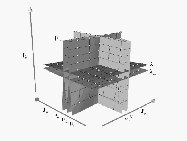
Figure 17: a) Transition of the WKB lattice upon crossing the intersection line of the separtrix surfaces in action space. The intersection line is represented as the “cross-ray”. b) Fig. 17a from behind.

6 Degenerate Ellipsoids

So far we treated the billiard in the general triaxial ellipsoid in its classical, quantum mechanical, and semiclassical aspects. The triaxial ellipsoid degenerates into simpler systems when any two or even all of the semiaxes coincide. In the latter case we obtain the sphere, in the former case prolate or oblate ellipsoids which are rotationally symmetric about the longer or shorter semiaxis, respectively. In this section we want to take a short look at these degenerate cases where the focus is on the similarities in the classical, quantum mechanical, and semiclassical treatment.

The main theme is that the coalescence of semiaxes of the ellipsoid induces the collision of roots or poles. In the classical treatment the disappearence of certain types of motions is expressed by the fact that some roots of a hyperelliptic curve collide and the genus of the curve drops. In the quantum mechanical treatment it is the singularities of the Helmholtz equation that coalesce, which is usually called confluence. Let us look at these transitions in more detail.

First of all we discuss the ellipsoid itself, without any dynamics. The general ellipsoid with parameteres $0<b<a<1$ has the semiaxes $1>\sqrt{1-b^{2}}>\sqrt{1-a^{2}}$. There are two choices of degenerate cases, either $b=a$ or $b=0$. For $b=a$ the longest semiaxes is $1$ and the two shorter semiaxes coincide, which gives the prolate ellipsoid. In the case $b=0$ the shorter semiaxis $\sqrt{1-a^{2}}$ is singled out and we obtain an oblate ellipsoid. If $a=b=0$ we obtain the sphere.

The algebraic treatment of the degenerate cases for the classical dynamics is quite simple. In the general case the hyperelliptic curves ${\cal R}_{w}$ have four fixed roots at $0<b<a<1$ and two movable roots (i.e. depending on the initial conditions) $0\leq s_{1}\leq a$ and $b\leq s_{2}\leq 1$ with $s_{1}\leq s_{2}$. Placing the movable roots $s_{i}$ into the three intervals marked by the fixed roots we obtain four possibilities, corresponding to the four types of motion.

Let us first consider the prolate case where $b=a$ and the $\eta$-range has vanished. In terms of the ranges for $\xi$ and $\zeta$ only case $P$ remains, because the other three become special cases of it, see Fig. 11. Only the ordering of the roots $0\leq s_{1}^{2}\leq a^{2}\leq s_{2}^{2}\leq 1$ is left which means that there is only one type of motion in the prolate ellipsoid. The genus of the hyperelliptic curve has dropped to one and the remainder of the $\eta$-interval is a pole at $z=a^{2}$, i.e. the integral in Eq. (50) is elliptic and of the third kind. Integrating around this pole gives the residue of this pole divided by $2\pi$, which is

$$I_{\eta}=I_{\mu}=\pm\sqrt{K^{2}-L^{2}-2a^{2}E}=L_{x}.$$ (122)

This is the angular momentum of the rotational degree of freedom, which is itself an action because the corresponding angle is cyclic. Hence even though the $\eta$-interval disappears, the $\eta$-action of course does not, this is the reason for the “appearance” of the pole.

In the oblate case $b=0$ the $\zeta$-interval vanishes so that in terms of the ranges for $\xi$ and $\eta$ the two cases $OA$ and $OB$ remain with the corresponding orderings of the roots $0\leq s_{1}^{2}\leq s_{2}^{2}\leq a^{2}$ and $0\leq s_{1}^{2}\leq a^{2}\leq s_{2}^{2}\leq 1$, respectively. $O$ becomes a special case of $OA$ and $P$ a special case of $OB$, see Fig. 11. Again the hyperelliptic curve attains a double root, so the genus drops and we obtain an elliptic differential of the third kind. The residue at the pole at $z=b=0$ gives $2\pi I_{\nu}$, where $I_{\nu}$ is the angular momentum about the symmetry axis; we find

$$I_{\zeta}=I_{\nu}=L=L_{z}.$$ (123)

If we finally collapse to the sphere with $b=a=0$, there is only the $\xi$-interval left. The motion in this interval describes the radial dynamics. The genus of the curve has dropped to 0, because now $s_{1}$ is fixed at zero. The two angular degrees of freedom are hidden in a pole at 0. Considering Eq. (13) we see that $l=0$ for $a=b=0$ so that in this case we find

$$I=I_{\nu}+I_{\mu}=K=|{\mbox{\boldmath$L$\unboldmath}}|.$$ (124)

The fact that there is only one pole while we would like to obtain two actions can be taken as an indication that the system is now degenerate, i.e. it has more constants of motion than degrees of freedom.

Let us now consider the separated Helmholtz equation. The partial fraction decomposition of $g/f$ in Section 4 shows that we have regular singular points at $\pm a$ and $\pm b$ in the case of a general ellipsoid. The solutions with exponents $1/2$ and $0$ gave the different parities. In the prolate case we have a confluence of $a$ with $b$ and of $-a$ with $-b$. The equations for $\xi$ and $\zeta$ reduce to the prolate spheroidal wave equations. Scaling the variables according to $\xi=a\tilde{\xi}$ and $\zeta=a\tilde{\zeta}$ gives them the familiar appearance (see [39])

$$(\tilde{\xi}^{2}-1)\psi^{\prime\prime}+2\tilde{\xi}\psi^{\prime}-(\lambda-c^{2}\tilde{\xi}^{2}+\frac{m^{2}}{\tilde{\xi}^{2}-1})\psi = 0,$$ (125)

$$(1-\tilde{\zeta}^{2})\psi^{\prime\prime}-2\tilde{\zeta}\psi^{\prime}+(\lambda-c^{2}\tilde{\zeta}^{2}-\frac{m^{2}}{1-\tilde{\zeta}^{2}})\psi = 0$$ (126)

with parameters

$$\lambda=(4kE-2a^{2}E)/\hbar^{2},\quad c=2a^{2}E/\hbar^{2},\quad m^{2}=L_{x}^{2}/\hbar^{2}.$$ (127)

The variable $\eta$ can be turned into an angle after some scaling to compensate for the vanishing of the $\eta$-range. The corresponding differential equation yields the familiar result $m\in{\mathbb{Z}}$ which means that each energy eigenvalue is twofold degenerate. Equations (125) and (126) are identical. The way of writing them just indicates that they are considered on the different ranges $\tilde{\zeta}\in[-1,1]$ and $\tilde{\xi}\geq 1$. The indicial equations for the regular singular points $\tilde{\xi}=\pm 1$ and $\tilde{\zeta}=\pm 1$ are of course the same and give the exponents $\pm\alpha=m/2$. Note that half the residue of the classical action integral over the coalesced singularity gives the exponent of the indicial equation in the quantum case.

For the oblate case $b=0$ we obtain a confluence of $b$ with $-b$ which gives a regular singular point at $0$ for the equations for $\xi$ and $\eta$. The two regular singular points at $\pm a$ usually are removed by transforming $\xi$ and $\eta$ separately according to $\xi^{2}=a^{2}+a^{2}\tilde{\xi}^{2}$ and $\eta^{2}=a^{2}-a^{2}\tilde{\eta}^{2}$. This gives the familiar pair of oblate spheroidal wave equations (see again [39])

$$(\tilde{\xi}^{2}+1)\psi^{\prime\prime}+2\tilde{\xi}\psi^{\prime}-(\lambda-c^{2}\tilde{\xi}^{2}-\frac{m^{2}}{\tilde{\xi}^{2}+1})\psi = 0,$$ (128)

$$(1-\tilde{\eta}^{2})\psi^{\prime\prime}-2\tilde{\eta}\psi^{\prime}+(\lambda+c^{2}\tilde{\eta}^{2}-\frac{m^{2}}{1-\tilde{\eta}^{2}})\psi = 0$$ (129)

with $\lambda$ and $c^{2}$ again defined as in Eq. (127) but now $m^{2}=L_{z}^{2}/\hbar^{2}$. Similarly to the prolate case the variable $\zeta$ can be turned into an angle and the corresponding equation again gives $m\in{\mathbb{Z}}$, i.e. the twofold degeneracy of the energy eigenvalues. The indicial equations for the regular singular points $\tilde{\xi}=\pm i$ and $\tilde{\eta}=\pm 1$ which correspond to the original regular singular points $\xi=0$ and $\eta=0$ are again the same and again give the exponents $\alpha=\pm m/2$. For the sphere let $a=b=0$ which gives $l=0$. The scaling $\xi=r\hbar/\sqrt{2E}$ then turns the equation for $\xi$ into

$$r^{2}\psi^{\prime\prime}+2r\psi^{\prime}+(r^{2}-n(n+1))\psi=0$$ (130)

with $n(n+1)=|{\mbox{\boldmath$L$\unboldmath}}|^{2}/\hbar^{2}$. The variables $\eta$ and $\zeta$ can be transformed into the azimutal and polar angles of the sphere and the corresponding equations give the familiar result $n\in{\mathbb{N}}_{0}$ and the $(2n+1)$-fold degeneracy of the energy eigenvalues. Eq. (130) obviously is the defining equation for spherical Bessel functions. It has a regular singular point at $0$ with exponents $n$ and $-(n+1)$. The corresponding solutions are the so called spherical Bessel functions of first and second kind. The asymptotics at $0$ picks out the functions of first kind as the physical solutions for the sphere.

Note that all the equations cited here for the degenerate cases have an irregular singular point at $\infty$. In the non-degenerate case $\infty$ is a regular singular point of Eq. (56).

Concerning the separation of the separation constants the non-degenerate Helmholtz equation presents the worst case because it is not separable in the separation constants. In the prolate and oblate cases only the constant $m$ can be separated off, the equations are called partially separable for separation constants. The billiard in the sphere belongs to the simplest class of equations which are completely separable for separation constants.

For the semiclassical treatment it is again illuminating to have a look at what happens to the hyperelliptic curve ${\cal R}_{w}$ in the degenerate cases. In the non-degenerate case ${\cal R}_{w}$ has genus 2 and therefore has two complex periods giving the penetration integrals $\Theta_{\xi}$ and $\Theta_{\zeta}$ in Equations (53) and (54). In the prolate and oblate limiting cases one of the handles in Fig. 9 vanishes. The genus of the curve drops to 1, i.e. the curve becomes elliptic. Generally an elliptic curve has one complex period that gives one penetration integral. In our case it is more useful to think of the elliptic curves for the prolate and oblate cases as singular limits of a hyperelliptic curve for the following reasons. During the prolate limiting process the middle handle in Fig. 9 shrinks. The penetration integrals are not only defined for any $b<a$ but even for $a=b$ where they become infinite. This means that although the curve corresponding to the prolate billiard motion is elliptic there is no tunneling in our semiclassical treatment. During the oblate limiting process the upper handle in Fig. 9 shrinks. Again the penetration integrals are even defined for the limiting case $b=0$ where the curve becomes elliptic. Here $\Theta_{\zeta}$ diverges and $\Theta_{\xi}$ stays finite. The prolate and the oblate limiting cases have in common that the penetration integrals connected to the vanishing handle diverge. But the oblate billiard still has one finite penetration integral that gives the semiclassical description of the tunnelling between tori corresponding to the two types of motions present here. This is why the oblate limiting behaviour may be considered as the more typical case. The prolate ellipsoidal billiard is peculiar in this sense. This peculiarity is also reflected by the fact that the prolate ellipsoidal billiard exhibits quantum monodromy, see [40]. From the point of view of periods of the Riemann surface it is important to mention that in the prolate case the sum of the penetration integrals is finite.

The degeneracy of the energy eigenlevels can semiclassically be understood by inspection of the energy surfaces. In the prolate and oblate cases the energy surface is symmetric with respect to the sign change of the action corresponding to the conserved angular momentum [7]. Thus the EBK quantization condition is each time fulfilled simultaneously at two points of the energy surface. The additional degeneracy of the billiard in the sphere classically manifests itself in the resonance of the azimutal and polar angular motion. The ratio of the corresponding frequencies has modulus 1, see [7]. The energy surface is thus foliated by straight lines what makes the EBK quantization condition being fulfilled not only at one point of the energy surface but on a whole line of points. This gives the $(2n+1)$-fold degeneracy of the energy eigenlevels.

7 Conclusions and Outlook

The last section demonstrated the unity of classical, semiclassical and quantum mechanical treatment in the complex plane, which is one main aspect of this exposition. Another one is to emphasize the simple and nice picture of the quantum mechanics of an integrable system as a discretization of classical action space. Away from the separatrix surfaces the discretization gives regular lattices due to the applicability of the simple EBK quantization of Liouville-Arnold tori in Eq. (4). It is much harder to give a semiclassical description of the quantum states whose eigenvalues in action space lie close to the separatrix surfaces because of the presence of quantum mechanical tunneling between tori with different Maslov indices. The tunneling was incorporated by a uniform WKB quantization scheme. This approach is necessary because the application of the simple quantization rule (4) close to the separatrix surfaces in action space can give erroneous additional eigenstates [32]. The ingredients for the WKB quantization scheme, i.e. the three classical actions and the two penetration integrals, have a consistent interpretation as the real and purely imaginary periods of a single Abelian differential of second kind on a hyperelliptic curve of genus 2. In this sense quantum mechanics appears as a “complexification” of classical mechanics.

For the billiard in the ellipsoid we were able to represent all quantum states as a regular WKB lattice in the space of the slightly modified actions $J$ which are twice the actions $\tilde{\mbox{\boldmath$I$\unboldmath}}$ of the symmetry reduced system. This is impossible in the space of the original actions $I$. The two classical senses of rotations of motion types $P$, $OA$, and $OB$ give two different tori in phase space whose actions differ in sign. Quantum mechanically we cannot distinguish between these tori and it is therefore impossible to assign different quantum state to them. In [10] all systems like the ellipsoidal billiard which (after some symmetry reduction) allow for a representation of the eigenvalues in action space are refered to as “one-component systems”. In order to represent quantum states in action space it is generally necessary to modify the original actions. For systems which are no one-component systems the WKB lattice will be much less regular then.

For future work on ellipsoidal quantum billiards we want to mention two directions. On the one hand the ellipsoidal quantum billiard can be taken as the starting point for computations of non-integrable quantum billiards resulting from slight distortion of the ellipsoidal boundary. On the other hand the semiclassical analysis in terms of periodic orbits is still to be worked out. For a chaotic system the Gutzwiller trace formula gives a semiclassical expression for the quantum density of states as a summation over isolated periodic orbits [41, 42, 43]. Analogously the quantum density of states of an integrable system can semiclassically be written as a summation over resonant tori, i.e. over families of periodic orbits. The Berry-Tabor trace formula gives the quantum density of states of an integrable system with $f$ degrees of freedom as a summation over resonant $f$-tori [44]. The main contribution to the density of states stem from the shortest periodic orbits. Generally the shortest periodic orbits do not foliate $f$-tori but lower dimensional tori. Since these contributions are not included in the generic case discussed in [44] they demand special considerations [45]. In addition to that the presence of separatrices demands a modification of the Berry-Tabor trace formula [32]. Both the non-generic contributions of resonant 2-tori and of isolated periodic orbits, and the presence of the crossing separatrices complicate the periodic orbit summation for ellipsoidal quantum billiards. For three-dimensional billiards as models for nuclei the shortest periodic orbits are important for the explanation of shell structures. For rotationally symmetric billiards this is considered in [46, 47]. For non-symmetric ellipsoids this is still to be done.

References

- [1] C. G. J. Jacobi. Vorlesungen über Dynamik. Chelsea Publ., New York, 1969.
- [2] B. A. Dubrovin. Theta functions and non-linear equations. Uspehki Mat. Nauk, 36(2):11–80, 1981.
- [3] M. V. Berry. Regularity and chaos in classical mechanics, illustrated by three deformations of a circular ’billiard’. Eur. J. Phys., 2:91–102, 1981.
- [4] P. H. Richter. Die Theorie des Kreisels in Bildern. Report 226, Institut für Dynamische Systeme, 1990.
- [5] H. R. Dullin, M. Juhnke, and P. H. Richter. Action integrals and energy surfaces of the Kovalevskaya top. Bifurcation and Chaos, 4(6):1535–1562, 1994.
- [6] H. R. Dullin. Die Energieflächen des Kowalewskaja-Kreisels. Mainz Verlag, Aachen, 1994. Dissertation.
- [7] P. H. Richter, A. Wittek, M. P. Kharlamov, and A. P. Kharlamov. Action integrals for ellipsoidal billiards. Z. Naturforsch., 50a:693–710, 1995.
- [8] J. Wiersig and P.H. Richter. Energy surfaces of ellipsoidal billiards. Z. Naturforsch., 51a:219–241, 1996.
- [9] H.-P. Schwebler. Invarianten in Systemen mit schwacher Dissipation. Dissertation, Universität Bremen, 1997.
- [10] J. Wiersig. Die klassische und quantenmechanische Beschreibung integrabler Hamiltonscher Systeme im Wirkungsraum. Dissertation, Universität Bremen, 1998.
- [11] O. Heudecker. Teilchenbewegung in der Kerr-Raumzeit. Dissertation, Universität Bremen, 1995.
- [12] H. R. Dullin, O. Heudecker, M. Juhnke, H. Pleteit, H.-P. Schwebler, H. Waalkens, J. Wiersig, and A. Wittek. Energy surfaces in action space. Report 406, Institut für Dynamische Systeme, 1997.
- [13] J. B. Keller. Corrected Bohr-Sommerfeld quantum conditions for nonseparable systems. Ann. Phys. (NY), 4:180–188, 1958.
- [14] V. I. Arnold. Mathematical Methods of Classical Mechanics, volume 60 of Graduate Texts in Mathematics. Springer, Berlin, 1978.
- [15] A. Einstein. Zum Quantensatz von Sommerfeld und Epstein. Verh. DPG, 19:82–92, 1917.
- [16] H.-J. Stöckmann and J. Stein. Quantum chaos in billiards studied by microwave absorption. Phys. Rev. Lett., 64:2215, 1990.
- [17] J. Stein and H.-J. Stöckmann. Experimental determination of billiard wave functions. Phys. Rev. Lett., 68:2867, 1992.
- [18] H. Alt, H.D. Gräf, H.L. Harney, R. Hofferbert, H. Lengeler, C. Rangacharyulu, A. Richter, and P. Schardt. Superconducting billiard cavities with chaotic dynamics : An experimental test of statistical measures. Phys. Rev. E, 50:1, 1994.
- [19] U. Dörr, H.-J. Stöckmann, M. Barth, and U. Kuhl. Scarred and chaotic field distributions in three-dimensional sinai-microwave resonators. Phys. Rev. Lett., 80:1030, 1998.
- [20] V.M. Strutinsky, A.G. Magner, S.R. Ofengenden, and T. Døssing. Semiclassical interpretation of the gross-shell structure in deformed nuclei. Z. Phys. A, 283:269–285, 1977.
- [21] M. Brack. The physics of simple metal clusters: self-consistent jellium model and semiclassical approaches. Rev. Mod. Phys., 65:677–732, 1993.
- [22] C. Gmachl, F. Capassa, E. E. Narimanov, J. U. Nöckel, A. D. Stone, J. Faist, D. L. Sivco, and A. Y. Cho. High-power directional emission from microlasers with chaotic resonantors. Science, 280:1556, 1998.
- [23] Y. Ayant and R. Arvieu. Semiclassical study of particle motion in two-dimensional and three-dimensional elliptical boxes: I. J. Phys. A: Math. Gen., 20:397–409, 1987.
- [24] Y. Ayant and R. Arvieu. Semiclassical study of particle motion in two-dimensional and three-dimensional elliptical boxes: II. J. Phys. A: Math. Gen., 20:1115–1136, 1987.
- [25] R. Arvieu, F. Brut, J. Carbonell, and J. Touchard. Phase-space organizations in prolate und oblate potentials: Classical, semiclassical, and quantum results. Physical Review A, 35(6):2389–2408, 1987.
- [26] Herbert Goldstein. Classical Mechanics. Addison-Wesley, Reading, MA, 2 edition, 1980.
- [27] I. S. Gradshteyn and I. M. Ryzhik. Tables of Integrals, Series, and Products. Academic Press, New York, 1965.
- [28] P.M. Morse and H. Feshbach. Methods of Theoretical Physics. McGraw-Hill, New York, 1953.
- [29] Paul F. Byrd and Morris D. Friedman. Handbook of Elliptic Integrals for Engineers and Physicists. Springer, Berlin, 1971.
- [30] W. Ludwig and C.. Falter. Symmetries in Physics. Springer, Berlin, 1988.
- [31] E. T. Whittaker and G. N. Watson. A Course of Modern Analysis. Cambridge University Press, Cambridge, 4 edition, 1965.
- [32] H. Waalkens, J. Wiersig, and H. R. Dullin. The elliptic quantum billiard. Ann. Phys., 260(1):50–90, 1997.
- [33] William H. Press, Brian P. Flannery, Saul A. Teukolsky, and William T. Vetterling. Numerical Recipes in C. The Art of Scientific Computing. Cambridge University Press, Cambridge, 1988.
- [34] M. V. Berry and K. E. Mount. Semiclassical wave mechanics. Rep. Prog. Phys., 35:315–397, 1972.
- [35] W.H. Miller. Semiclassical treatment of multiple turning-point problems - phase shifts and eigenvalues. J. Chem. Phys., 48(4):1651–1658, 1968.
- [36] J. N. L. Connor. On the analytical description of resonance tunnelling reactions. Mol. Phys., 15(1):37–46, 1968.
- [37] M. S. Child. Semiclassical theory of tunneling and curve-crossing problems: a diagrammatic approach. J. Mol. Spectroscopy, 53:280–301, 1974.
- [38] P. H. Richter, H. R. Dullin, H. Waalkens, and J. Wiersig. Spherical pendulum, actions and spin. J.Chem.Phys., 100:19124–19135, 1996.
- [39] Milton Abramowitz and Irene A. Stegun. Handbook of Mathematical Functions. Dover Publications, New York, 1965.
- [40] H. Waalkens and H. R. Dullin. Quantum monodromy in prolate ellipsoidal billiards. (in preparation), 1998.
- [41] M. C. Gutzwiller. Phase-integral approximation in momentum space and the bound states of an atom. J. Math. Phys., 8(10):1979–2001, 1967.
- [42] M. C. Gutzwiller. Energy spectrum according to classical mechanics. J. Math. Phys., 11(6):1791–1806, 1970.
- [43] M. C. Gutzwiller. Periodic orbits and classical quantization conditions. J. Math. Phys., 12(3):343–358, 1971.
- [44] M. V. Berry and M. Tabor. Closed orbits and the regular bound spectrum. Proc. R. Soc. Lond. A, 349:101–123, 1976.
- [45] S. C. Creagh and R. G. Littlejohn. Semiclassical trace formulas in the presence of continuous symmetries. Phys. Rev. A, 44(2):836–850, 1991.
- [46] H. Frisk. Shell structures in terms of periodic orbits. Nuclear Physics, A511:309–323, 1990.
- [47] A.G. Magner et. al. Semiclassical analysis of shell structure in large prolate cavities. Ann. Phys., 6:555–594, 1997.