Temporal intermittency and cascades in shell models of turbulence

Abstract

The 2d and 3d like Gletzer, Okhitani and Yamada (GOY) shell models are examined. The 2d like model shows a transition from statistical quasi-equilibrium to cascade of enstrophy as a function of the spectral ratio of energy to enstrophy. The transition is related to the ratio of time scales, corresponding to eddy turnover times, between shells. The anomalous scaling, giving rise to non-linear scaling functions, is also connected to the ratio of eddy turnover times. This is illustrated in a simple stochastic model, where the structure function, $\zeta(q)$, becomes independent of $q$. In the 3d like model the multiscaling is also influenced by the existence of a second non-positive definite inviscid invariant, the helicity.

The problem of understanding the scaling properties of velocity correlations in isotropic and homogeneous turbulence is still largely unsolved. The only exact derived property is the Kolmogorov scaling law for the third order moments, $C_{3}(r)=-4\epsilon r/5+6\nu dC_{2}(r)/dr$, where $C_{q}(r)\equiv\langle\Delta v(r)^{q}\rangle=\langle|v(x+r)-v(r)|^{q}\rangle,r$ is the distance in the fluid and $\langle.\rangle$ is the ensamble average. This relation is not closed, since it contains both second and third order correlation functions. In the inertial range defined by, $L\gg r\gg\lambda$, where $L$ is the outer scale and $\lambda$ the inner or Kolmogorov dissipation scale, the second term on the right hand side is negligible and the scaling relation, $C_{3}(r)\sim r^{\zeta(3)}$, with $\zeta(3)=1$, holds. The classical Kolmogorov theory (K41) based on dimensional arguments states that $C_{q}(r)\sim r^{\zeta(q)}$, with $\zeta(q)=q/3$. It was noted by Landau shortly after the theory was presented that the energy dissipation could vary so much as to alter the scaling laws. This was incorporated in a refined version of Kolmogorovs theory (K62), in which a dependence on $L/r$, the ratio of the outer scale to the scale in the inertial range was incorporated.

It has been seen in numerous experiments that $\zeta(q)$ is a weakly non-linear function of $q$, different from the Kolmogorov predictions for $q$ different from 3. It follows from the Hølder inequality that $\zeta(q)$ is a convex of $q$, thus $\zeta(q)>q/3$ for $q<3$ and $\zeta(q)<q/3$ for $q>3$. The deviation of the scaling from the K41 prediction is referred to as intermittency corrections. It is widely attributed to the fact that the energy dissipation in fully developed turbulence is indeed highly inhomogeneous, basically taking place on lower dimensional subsets, filaments, of the flow field.

Numerical studies of the GOY shell model [1] of turbulence have been popular resently, mainly because this model, in which scaling relations completely equivalent to those of turbulence, also shows intermittency corrections to the K41 - equivalent - predictions. The GOY model structually resembles the spectral form of the Navier-Stokes equation, but there is no spatial fields associated with the wave components in the GOY model. The intermittency corrections in the scaling properties are thus associated with temporal intermittency which can only be weakly linked to spatial intermittency through the Taylor hypothesis. The connection between the spatial intermittency of turbulence and temporal intermittency of the GOY model is not clear, but the hope is that understanding the latter can shed light upon the former. This note is about the latter.

In the GOY model the spectral domain is represented as shells, each of which is defined by a wavenumber $k_{n}=\lambda^{n}$, where $\lambda$ is a scaling parameter defining the shell spacing. There are $2N$ degrees of freedom, where $N$ is the number of shells, namely the generalized complex shell velocities, $u_{n}$ for $n=1,N$. The dynamical equation for the shell velocities is,

$$\dot{u}_{n}=ik_{n}(u_{n+2}u_{n+1}-\frac{\epsilon}{\lambda}u_{n+1}u_{n-1}+\frac{(\epsilon-1)}{\lambda^{2}}u_{n-1}u_{n-2})^{*}-\nu k_{n}^{2}u_{n}+f\delta_{n,n_{0}},$$ (1)

where the first term represents the non-linear wave interaction or advection, the second term is the dissipation, and the third term the forcing, where $n_{0}$ is some small wavenumber. The boundary conditions are, $u_{-1}=u_{0}=u_{N+1}=u_{N+2}=0$. The model has two quadratic inviscid invariants, which are constants of motion in the case $f=\nu=0$, $E=\sum_{n}|u_{n}|^{2}$, referred to as the energy, and $H=\sum_{n}(\epsilon-1)^{-n}|u_{n}|^{2}$. For $\epsilon<1$ $H$ is non-positive definite, referred to as the helicity, and the model is thought of as modeling 3d turbulence. For $\epsilon>1$ $H$ is positive definite, referred to as the enstrophy, and the model is meant to resemble 2d turbulence. Dimensional arguments similar to those of K41 can be applied to the GOY model assuming dissipation of one of the conserved quantities. For the 2d type model, $1<\epsilon<2$, enstrophy will be dissipated, and an additional large scale drag term, $-\nu^{\prime}k_{n}^{-2}u_{n}$, is added to (1) in order to remove the energy. The reason for the enstrophy and not the energy being dissipated is the usual that the dissipation of energy is $k_{n}^{-\alpha}$ times the dissipation of enstrophy at shell $n$, thus negligible for $\alpha>0$ and $n\rightarrow\infty$. The Kolmogorov scaling for the 2d type model then becomes, $\langle|u_{n}|\rangle\sim k_{n}^{-(\alpha+1)/3}$. Note that this is an unstable fixed point of (1) for $f=\nu=0$, describing a cascade. As pointed out by Aurell et al. [2] in the case of $\alpha=2$ this scaling coincides with the scaling that would be obtained in a statistical equilibrium, in which the enstrophy is distributed evenly among the degrees of freedom of the system, $\langle|u_{n}|\rangle\sim k_{n}^{-\alpha/2}$. The $\alpha=2$, corresponding to $\epsilon=5/4$, case is a borderline case between models showing cascade, for $\alpha<2$, and models showing statistical (quasi-)equilibrium, for $\alpha>2$. In order to show this a series of numerical model runs for different values of $\epsilon$ have been performed, details of which are reported elsewhere [3].

FIG. 1.: Results of runs of the 2d like GOY model for different values of $\epsilon$. Shown is the spectral slope $\gamma=-\log(\langle u\rangle)/\log(k)$ as function of $\alpha=-\log(\epsilon-1)/\log(\lambda)$. The lines are the Kolmogorov scaling for enstrophy cascade and equipartitioning of enstrophy, respectively. For the 2d like GOY models an additional dissipation of the form, $-\nu^{\prime}k_{n}^{-2}u_{n}$, is applied in order to remove energy at small wave number shells. The model is run with $n=50,k_{0}=\lambda^{-4},\lambda=2,f_{n}=5\times 10^{-4}\times(1+i)\delta_{n,15},(\epsilon=11/10,\nu=5\times 10^{-27},\nu^{\prime}=100),(\epsilon=117/100,\nu=5\times 10^{-27},\nu^{\prime}=100),(\epsilon=5/4,\nu=5\times 10^{-25},\nu^{\prime}=100),(\epsilon=3/2,\nu=5\times 10^{-23},\nu^{\prime}=100),(\epsilon=7/4,\nu=5\times 10^{-23},\nu^{\prime}=100),(\epsilon=2,\nu=5\times 10^{-20},\nu^{\prime}=100).$ The models show a cross-over at $\alpha=2$ between statistical equilibrium, $\alpha>2$, and enstrophy cascading, $\alpha<2$.

Figure 1 shows the spectral slopes obtained. The two lines shows the slopes corresponding to cascade and statistical equilibrium respectively, the diamonds are the numerical results. The figure clearly shows a cross-over from one type of behavior to the other. The reason for this transition is related to the scaling of typical timescales, or eddy turnover times, for the different shells. The eddy turnover time at shell $n$ is given as $\tau_{n}=(k_{n}\langle|u_{n}|\rangle)^{-1}$ as seen from (1) or dimensional arguments. The eddy turnover time then becomes, $\tau_{\mbox{{cascade}}}\sim k^{(\alpha-2)/3}$ and $\tau_{\mbox{{equilibrium}}}\sim k^{(\alpha-2)/2}$ respectively. Thus for $\alpha>2$ the eddy turnover times in both cases increase with wave number, and equilibration via inverse enstrophy transfer, from large wave numbered shells to small wave numbered shells takes place. For $\alpha<2$ the situation is reversed, and a statistical equilibrium can newer be achieved. Similar results have been found by Yamada and Ohkitani [4] for a slightly different set of GOY models, with only one positive definite inviscid invariant, reffered here to as 3D type models.

In the 3d type models the situation is totally different, in this case the second inviscid invariant, the helicity, is not cascaded even though the ratio of absolute value of the helicity to the energy at shell $n$ grows exponentially with $n$ as is the case for the enstrophy. The reason is that the helicity has alternating signs for even and odd numbered shells. Therefore there will be a net production of (positive sign) helicity at odd numbered shells due to the dissipation, and no net flow of helicity from small wave number shells to large wave number shells is necessary. It has been demonstrated numerically that helicity is indeed the quantity to be cascaded in the (pathological) case of hyperviscosity only active on the outermost shell [5]. In the usual 3d case energy will be cascaded, with the resulting spectral scaling, $\langle|u|^{3}\rangle\sim k^{-1}$.

Both the 2d and the 3d models shows intermittency corrections to the Kolmogorov scaling depending on $\epsilon$ and $\lambda$. In this note I will suggest two different mechanisms in play in the 3d case, where only the one is in action in the 2d case.

In the 3d case it is observed that the structure function depends only on $\epsilon$ and $\lambda$ in the combination, $-\log(1-\epsilon)/\log(\lambda)=\alpha$ [6]. With $\delta\zeta(q)\equiv\zeta(q)-q/3$, $\delta\zeta(q)$ increases in absolute value when $\alpha$ increases. I suggest that this is due to differences in the ratio of helicity production and helicity elimination by dissipation at neighboring shells in the beginning of the dissipative subrange where scaling still approximately holds or where extended self-similarity can be applied [7]. This ratio, $r$, can be estimated as $r\equiv(\Delta H_{n-1}+\Delta H_{n+1})/2\Delta H_{n}\sim(\lambda^{-\alpha+2/3}+\lambda^{\alpha-2/3})/2$, which for $(\alpha,\lambda)=(0.5,2),(1,2),(2,2)$ gives $1.007,1.03,1.46$ respectively. So there is the biggest ”mis-match”, or non-cancellation, in the case $(2,2)$ where the biggest non-linearity in the structure function is observed. That these two things should be related is consistent with the findings of a moderated GOY model (model 3) by Benzi et al. [8], where 2 copies of the GOY model are coupled. In this model the helicity takes the form, $H=\sum_{n}k_{n}^{\alpha}(|u_{n}^{+}|^{2}-|u_{n}^{-}|^{2})$, where $u_{n}^{+}$ and $u_{n}^{-}$ are the two complex variables in shell $n$. In this model the helicity production and elimination will - on average - exactly balance, thus no dependence of the structure function on $\alpha$ should be expected in agreement with the numerical findings.

In the standard 3d case, $\alpha=1$, the structure function is still non-linear even though the above defined $r$ is close to 1. This is suggested to be due to the difference in time scales between the large and the small scales. This effect is expected also to determine the anomalous scaling in the 2d case, where only the dissipation of enstrophy plays a role. In the 2d case numerical studies suggests that the absolute size of $\delta\zeta(q)$ increases as $\alpha$ decreases from 2 to 0 [3]. This suggests that intermittency is enhanced with growing difference between eddy turnover times from one shell to the next, which goes as $\tau_{n+1}/\tau_{n}=\lambda^{(2-\alpha)/3}$.

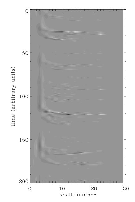
FIG. 2.: The non-linear transfer of energy from one shell to the next in the 3d like GOY model with $\epsilon=1/2$, all parameter values are standard, forcing is on shell number 4. The line segments pointing from shell $n$ at time $t$ to shell $n+1$ at time $t+\Delta t$ symbolize forward transfer, with magnitude proportional to the thickness of the line segment. Line segments pointing from shell $n+1$ at time $t$ to shell $n$ at time $t+\Delta t$ symbolizes backward transfer.

Figure 2 shows the non-linear transfer, $\Delta_{n}=k_{n-1}Im(u_{n-1}u_{n}u_{n+1})$ of energy from shell $n-1$ to shells $n$ and $n+1$ in the 3D case. The abscissa is the shell number and the ordinate is time, read from top to bottom, the figure is composed of line-segments connecting shells $n$ at time $t_{i}$ and shells $n+1$ at time $t_{i}+\Delta t$, symbolizing an energy transfer from shell $n$ in the time-interval $[t_{i};t_{i}+\Delta t]$. The thickness of the line-segment is proportional to the size of the transfer. Line-segments going from $n+1$ at time $t_{i}$ to $n$ at time $t_{i}+\Delta t$ symbolizes the inverse energy transfer. The figure shows that the transfer is temporally intermittent and occurring in bursts [9], with the transfer being faster as the bursts propagate to higher wave-number shells. From this the interpretation is straight forward; The residence time for a burst at a given shell is proportional to the eddy turnover time resulting in a more and more intermittent transfer as the eddy turnover time decreases. In order to illustrate how this kind of behavior can lead to anomalous scaling behavior, consider the following linear stochastic model, which is an extreme case.

Let $x_{n}$ be a stochastic variable representing the energy at shell $n$, governed by the dynamical equation;

$$x_{n}(t+1)=p_{n-1}(t)x_{n-1}(t)-p_{n}(t)x_{n}(t)-\nu k_{n}^{2}x_{n}(t)+f\delta_{n,1},$$ (2)

where $p_{n}$ is a stochastic variable which is 1 with probability $\tau_{N}/\tau_{n}$ and 0 with probability $1-\tau_{N}/\tau_{n}$, thus it represents a transition probability of energy transfer from shell $n$ to shell $n+1$. The boundary conditions are $x_{-1}=p_{N}=0$. The average residence time is then simply proportional to the eddy turnover time. It is easily seen that $x_{n}$ is always positive.

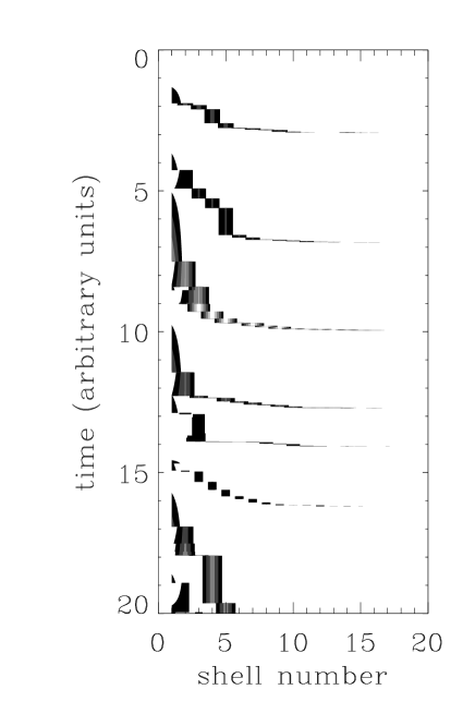
FIG. 3.: The result of a simulation of the simple stochastic model, $x_{n}$ is plotted as a function of time. The intermittent transfer is similar to what is seen in the GOY model, figure 2.

Figure 3 is similar to figure 2, but shows the values of $x_{n}$. There is obviously no inverse transfer in this model. By comparing figures 2 and 3 one sees that the intermittent structure of the transfers are similar. The energy will in this model scale inversely proportional to the eddy turnover time, so that if we identify $x_{n}$ with the energy/enstrophy of the GOY model $E_{n}=k_{n}^{\alpha}|u_{n}|^{2}$, the scaling of $\langle|u_{n}|\rangle\sim k_{n}^{-(\alpha+1)/3}$ is the same as for the GOY model. However, the structure function changes completely. It is readily calculated, with the result; $\langle x_{n}^{q}\rangle\sim k_{n}^{(\alpha-2)/3}x^{q}$, where $\tau_{n}=k_{n}^{(\alpha-2)/3}$ is the eddy turnover time at shell $n$ and $x=f\tau_{1}$ is the average energy input into the system during one large eddy turnover time. This means that the structure function, $\zeta(q)$, becomes independent of $q$. $q$ will only show up in the offset, $q\log(x)$ in a $\log\langle x_{n}^{q}\rangle$, $\log(k_{n})$ plot. This is illustrated in figure 4, showing the result of a numerical simulation.

FIG. 4.: Anomalous scaling behavior of the simple stochastic model. $\log(\langle x^{q}\rangle)$ vs. $\log(k)$ for $q=1,8$. The spectral slope does not depend on $q$, So that $\zeta(q)=(\alpha-2)/3$. The model was iterated for $10^{4}$ large eddy turnover times with $N=20,f=0.05,\nu=10^{-11}$.

Obviously this linear stochastic model cannot reproduce the scaling exponents of the GOY model or of real turbulence but it qualitatively illustrates the effect of temporal intermittency.

In conclusion, the behavior of the 2d like GOY model shows either statistical equilibrium or cascade of enstrophy depending on the ratio of the eddy turnover timescales between the shells. The dynamics and the multiscaling of the 3d like GOY model depends on the existence of the second non-positive definite inviscid invariant, helicity, through the way the helicity is dissipated in the model. In both cases, the multiscaling is an effect of temporal intermittency also originating from differences in eddy turnover times at the different scales, thus the 2d model with $\alpha=2$ shows no anomalous scaling. The effect is illustrated in a simple stochastic model. The scaling behavior of this simple model does not correspond to what is seen in the GOY model or in real turbulence. However, the model points to a mechanism of how the temporal intermittency can lead to anomalous scaling behavior. In order to further clarify the relationship between the spatial intermittency observed in turbulence and the temporal intermittency seen in these simple models, it would be interesting to see if the structures seen in the time - wave-number domain, figure 1, can be identified in direct numerical simulations of the Navier-Stokes equation.

Acknowledgements: It’s a pleasure to thank R. M. Kerr and J. Herring for valuable discussions and NCAR for hospitality and financial support. The work was granted by the Carlsberg foundation.

^† On leave from The Niels Bohr Institute, Department for Geophysics, University of Copenhagen, Juliane Mariesvej 30, DK-2100 Copenhagen O, Denmark.

REFERENCES

- [1] M. Yamada and K. Okhitani, J. Phys. Soc. of Japan 56, 4210 (1987); Progr. Theo. Phys. 79, 1265 (1988); Phys. Rev. Lett.. 60,983 (1988)
- [2] E. Aurell, G. Boffetta, A. Crisanti, P. Frick, G. Paladin and A. Vulpiani, Phys. Rev. E, 50, 4705, (1994).
- [3] P. D. Ditlevsen and I. A. Mogensen, Phys. Rev. E, 53, 4785, 1996.
- [4] M. Yamada and K. Okhitani, Phys. Lett. A, 134, 165, 1988.
- [5] P. D. Ditlevsen, Phys. Fluids, 9, 1482-1484, 1997.
- [6] R. Benzi, L. Kadanoff, D. Lohse, M. Mungan and J. Wang, Phys. Fluids 7, 617, 1995.
- [7] R. Benzi, S. Ciliberto, C. Baudet, G. R. Chavarria, Physica D. 80, 385, 1995.
- [8] R. Benzi, L. Biferale, R. M. Kerr and E. Trovatore, preprint chao-dyn/9510010 in PBB for non-linear science.
- [9] M. H. Jensen, G. Paladin and A. Vulpiani, Phys. Rev. A, 43, 798, 1991.