Fix-point Multiplier Distributions in Discrete Turbulent Cascade Models

Abstract

One-point time-series measurements limit the observation of three-dimensional fully developed turbulence to one dimension. For one-dimensional models, like multiplicative branching processes, this implies that the energy flux from large to small scales is not conserved locally. This then renders the random weights used in the cascade curdling to be different from the multipliers obtained from a backward averaging procedure. The resulting multiplier distributions become solutions of a fix-point problem. With a further restoration of homogeneity, all observed correlations between multipliers in the energy dissipation field can be understood in terms of simple scale-invariant multiplicative branching processes.

PACS: 47.27.Eq, 05.40.+j, 02.50.Sk
KEYWORDS: fully developed turbulence, multiplicative branching processes, multiplier distribution, fix-point behaviour

CORRESPONDING AUTHOR:
Martin Greiner
Max-Planck-Institut für Physik komplexer Systeme
Nöthnitzer Str. 38
D–01187 Dresden, Germany
tel.: 49-351-871-1218
fax: 49-351-871-1199
email: greiner @ mpipks-dresden.mpg.de

I Introduction

As the classic of multi-scale processes, fully developed Navier-Stokes turbulence remains to be a fortress, which besides many heroic attempts has not surrendered to the cohorts of theoretical physicists [1]. Hence, any progress in a thorough theoretical understanding should be data driven. This means that for a characterisation and better understanding of data there is first the need to develop simple heuristic models and to try to learn the most from them. Only then, with newly motivated and intriguing ideas and clever theoretical technology, a Trojan horse can be found to take this fortress by storm. – This paper is not about the still to be found Trojan horse. It is about the revelation of two pitfalls which appear during the early stage of its attempted construction.

The energy dissipation field in fully developed turbulence reveals striking, close to singular fluctuations. Empirically some features of these intermittent fluctuations can be reproduced by multiplicative branching models [2, 3, 4, 5]. Their particular strength lies in their simplicity and their inherent self-similarity, which proofs useful when discussing multifractal behaviour in the limit of a very large Reynolds number [6]. These models rely on two assumptions: (a1) the weight curdling, associated with the branchings and describing the energy flux from large to small scales, is scale-independent, and (a2) different branchings are independent of each other and are not correlated. Of course, these assumptions have been directly tested with large Reynolds number atmospheric and wind channel data [7, 8, 9, 10] and conclusions have been drawn that (b1) assumption (a1) appears to hold whereas (b2) assumption (a2) appears to be in conflict with the experimental findings, where correlations between different, reconstructed branchings have been observed. Although some modifications of the cascade models have been proposed to include these effects [8], many physicists think of it as a major drawback to the cascade models.

This criticism of the cascade models is by no means justified and this brings us back to the pitfall-business mentioned in the beginning. The immediate testing of the cascade model assumptions (a1) and (a2) from data is not as straightforward as had been long anticipated. In order to explain this point we have to understand how the measurements are done:

An anemometer records one component, which is usually longitudinal, of the velocity field as a time series in one point. Given that the fluctuation strength is small this time series can be interpreted as a one-dimensional spatial realisation of the velocity field at a fixed time; this is known as Taylors frozen flow hypothesis. Since the energy dissipation tensor is a functional of spatial derivatives of the velocity field, the spatial realisation of the streamwise component of the velocity field can be converted into a spatial realisation of the streamwise components of the energy dissipation tensor. It is the statistical properties of this one-dimensional energy dissipation field which are compared to, for example, the multiplicative cascade models. The important thing to note here is that the energy dissipation field is measured one-dimensional, but is generated from the three-dimensional dynamics of fully developed turbulence. If we assume a cascade dynamics to hold in three dimensions, then the energy flux from large to small scales is conserved in every three-dimensional branching. For a one-dimensional cut through the three-dimensional dynamics this, of course, needs not to hold. As a consequence, branchings used in one-dimensional multiplicative cascade models should not conserve the energy flux locally. Globally, that means on average, conservation of energy flux should be fulfilled. This then means, that the weights (or dynamical multipliers) used in the cascade evolution can not be reconstructed from the one-dimensional cut through the energy dissipation field resolved at the finest scale. With other words, the reconstructed multipliers obtained by smoothing from fine to large scales are not equal to the dynamical multipliers of the cascade evolution from large to fine scales.

A second pitfall occurring in the comparison of cascade models with data has already been noticed previously [11]: multiplicative cascade models lead to hierarchical structures which are not homogeneous. The time series measurements sketched above are unable to trigger on these hierarchical structures. Hence, homogeneity has to be restored in the cascade models first, before they are compared to data.

For a fair comparison between cascade models and data these two points have to be taken into account: (c1) no local conservation of energy flux in the branchings of one-dimensional multiplicative cascade models since they represent one-dimensional sections through an underlying three-dimensional cascade dynamics, and (c2) restoration of homogeneity in the hierarchical multiplicative cascade models. Taking these two points into consideration we will show in this Paper that multiplicative cascade models can be constructed, which still respect assumptions (a1) and (a2) and which at the same time are successful in explaining the presently available experimental observations (b1) and (b2).

The organisation of the Paper is as follows: In Sect. II we summarise the experimental facts about multiplicative cascade processes in fully developed turbulence. Section III already reveals that three-dimensional multiplicative cascade models, observed in one dimension, lead to fix-point solutions for the various reconstructed multiplier distributions which come close to the experimentally observed ones. Some analytical insight into the fix-point behaviour is given in Sect. IV. Sect. V considers three specific popular variants of one-dimensional multiplicative cascade models, the asymmetric binomial, the log-normal and the log-Poisson model, and studies the implications of our two points (c1) and (c2). Conclusions are given in Sect. VI.

II Experimental facts about turbulent cascade processes

A Discrete multiplicative branching processes

Multiplicative branching processes serve to model properties of the intermittent fluctuations observed in the energy dissipation field of fully developed turbulence. They relate the energy flux $E_{L}$ at some integral scale $L$ to $E_{r}=E_{L}W_{1}(\lambda)\cdots W_{J}(\lambda)$ contained in a subinterval of size $r=\lambda^{-J}$ at scale $J$ by a product of mutually independent random weights $W_{j}(\lambda)$. The length ratio $\lambda$ represents a free parameter; the most simple and most commonly chosen value is given by $\lambda=2$. Adopting also this latter choice and dropping the dependence of the random weights $W_{j}$ on $\lambda$, the multiplicative branching processes are from now on denoted as binary multiplicative cascade processes.

More precisely now, the energy flux $E_{k}^{(j)}$, contained in the interval $0\leq k<2^{j}$ with length $r=L/2^{j}$ splits into a left (L) and right (R) offspring interval, each of length $r/2$, whereby the content propagates according to $E_{2k}^{(j+1)}=W_{L}E_{k}^{(j)}$ and $E_{2k+1}^{(j+1)}=W_{R}E_{k}^{(j)}$, respectively. For each breakup the two random weights $W_{L,R}\geq 0$ are chosen, independently from any preceding breakup, according to a joint probability density $p(W_{L},W_{R})$. The splitting function, as we denote the latter, guarantees a full description of a binary breakup. For the special case where the splitting function is concentrated along the diagonal $W_{L}+W_{R}=1$, i.e. $p(W_{L},W_{R})=p(W_{L})\delta(W_{L}+W_{R}-1)$, each breakup strictly conserves energy flux. For all other forms the relation $E_{2k}^{(j+1)}+E_{2k+1}^{(j+1)}=E_{k}^{(j)}$ needs not to hold; however, on average it should hold.

A particular simple example is the binomial splitting function

$$p(W_{L},W_{R})=\frac{1}{2}\left[\delta(W_{L}-\frac{1+\alpha}{2})+\delta(W_{L}-\frac{1-\alpha}{2})\right]\delta(W_{L}+W_{R}-1)\quad,$$ (1)

which is known as the $p$-model [5]. Only two different local breakups are possible, each with the same probability. Here, energy flux is conserved for every local splitting.

In general, multiplicative cascade models are based on two assumptions: (a1) the existence of a scale-independent splitting function $p(W_{L},W_{R})$ and (a2) statistical independence of the random weights $W_{L,R}$ at one breakup from those of any other breakup. Once $p(W_{L},W_{R})$ is chosen, the assumptions (a1) and (a2) allow to determine all moments and scaling exponents of the energy dissipation $\varepsilon_{r}{=}E_{r}/r$ by inverse Laplace transforms [12, 13]. Many experimental measurements of moments and scaling exponents confirm that this simple construction reproduces the measured multifractal aspects of the energy dissipation field amazingly well (e.g. [6]).

B Experimental facts

From a theoretical point of view the various parametrisations suggested for the splitting function $p(W_{L},W_{R})$ serve to reproduce the scaling exponents observed in the one-dimensional cuts of the energy dissipation field, the latter being converted from velocity time series obtained from anemometers and employment of Taylors frozen flow hypothesis. Within the experimental error bars, such different models as the $p$-model [5], the log-normal model [14, 15], the log-Poisson model [16, 17, 18] and others are all capable to describe the observed scaling exponents. As a consequence of this model insensitivity some efforts have been taken to extract information about the splitting function directly from data [7, 8, 9]. In the following we will briefly sketch the operational procedure and summarise the essential results.

In the inertial range ($0\leq j\leq J$) the energy dissipation $\varepsilon(x,r)$ at length scale $r=L/2^{j}$ and position $x=kL/2^{j}$ is defined by

$$\varepsilon_{k}^{(j)}=\varepsilon\left(x=\frac{kL}{2^{j}},r=\frac{L}{2^{j}}\right)=\frac{1}{r}\int_{x}^{x+r}\varepsilon(x^{\prime})dx^{\prime}\quad,$$ (2)

where $0\leq k<2^{j}$. The experimentally measured ‘backward’ energies then become

$$\bar{E}_{k}^{(j)}=\frac{L}{2^{j}}\varepsilon_{k}^{(j)}=\sum_{l=k2^{J{-}j}}^{(k+1)2^{J-j}-1}E_{l}^{(J)}\quad.$$ (3)

They are obtained by successive summations from the finest resolution scale $J$ to larger ones and are generally not equal to the ‘forward’ energies $E_{k}^{(j)}$, which arise as intermediate states in the evolution of the cascade from larger to smaller scales. For a clearer distinction we denote the former with a bar. – Based on (3), so-called left, right and centred multipliers at scale $j$ and position $k$ are now operationally defined as

$$M_{k,L}^{(j)}=\frac{\bar{E}_{2k}^{(j+1)}}{\bar{E}_{k}^{(j)}},\quad M_{k,R}^{(j)}=\frac{\bar{E}_{2k+1}^{(j+1)}}{\bar{E}_{k}^{(j)}},\quad M_{k,C}^{(j)}=\frac{\bar{E}_{4k+1}^{(j+2)}+\bar{E}_{4k+2}^{(j+2)}}{\bar{E}_{k}^{(j)}}.$$ (4)

They may be denoted as base 2 multipliers, because the associated change of interval lengths refers to $\lambda=2$. They depend on the relative position of parent to offspring intervals. Multiplier distributions $p(M^{(j)})$ are obtained by histogramming all $0\leq k<2^{j}$ possible multipliers at a given scale and averaging over many realisations.

For cascade models with an energy flux conserving splitting function $p(W_{L},W_{R})=p(W_{L})\delta(W_{L}+W_{R}-1)$ the random weights $W_{L/R}$ are directly related to the multipliers $M_{L/R}$. Due to local energy flux conservation we have $E_{2k}^{(j+1)}+E_{2k+1}^{(j+1)}=(W_{k,L}^{(j)}+W_{k,R}^{(j)})E_{k}^{(j)}=E_{k}^{(j)}=\bar{E}_{k}^{(j)}$, so that the ‘forward’ energies $E_{k}^{(j)}$ are then identical to the ‘backward’ energies $\bar{E}_{k}^{(j)}$. Hence, $M_{k,L}^{(j)}=(W_{k,L}^{(j)}E_{k}^{(j)})/E_{k}^{(j)}=W_{k,L}^{(j)}$, and, analogously, $M_{k,R}^{(j)}=W_{k,R}^{(j)}$. For this case the multiplier distributions $p(M_{L/R}^{(j)})$ reproduce the scale-invariant splitting function $p(W_{L},W_{R})$.

Experimental analyses performed in atmospheric [7, 8] and wind tunnel turbulence [9] have revealed that within the inertial regime the multiplier distributions $p(M_{L/R}^{(j)})$ are to a very good degree independent of the length scale. The following parametrisation has been found empirically [8]:

$$p(M_{L/R})=\frac{\Gamma(2\beta)}{\Gamma(\beta)^{2}}\left[M_{L/R}(1-M_{L/R})\right]^{\beta-1}\quad,$$ (5)

where $\Gamma$ stands for the gamma function and where $\beta\approx 3.2$. See Fig. 1. In order to link this scale-invariant multiplier distribution directly to a splitting function, local energy flux conservation in each binary breakup of the cascade process has to be assumed. This then leads to

$$p(W_{L},W_{R})=\frac{\Gamma(2\beta)}{\Gamma(\beta)^{2}}\left[W_{L}W_{R}\right]^{\beta-1}\delta\left(W_{L}+W_{R}-1\right)$$ (6)

and the assumption (a1) of Sect. II.A of the existence of a scale-independent splitting function for multiplicative cascade models appears to be confirmed. Notice, however, that the additional assumption of local energy flux conservation had to be employed to convert the multiplier distribution (5) into the splitting function (6).

What about assumption (a2) of Sect. II.A? If the multipliers $M_{k,L/R}^{(j)}$ are independent from those at other scales and positions, as required from the multiplicative cascade models, then the conditional multiplier distributions $p(M_{2k(+1),L/R}^{(j+1)}|M_{k,L/R}^{(j)})$, which correlate an offspring multiplier with its parent multiplier, should not depend on the latter, i.e. $p(M_{2k(+1),L/R}^{(j+1)}|M_{k,L/R}^{(j)})=p(M_{2k(+1),L/R}^{(j+1)})$. The experimental findings, however, indicate a dependency (see Fig. 1): given a small parent multiplier $M_{k,L/R}^{(j)}\leq 1/2$ the conditional multiplier distribution $p(M_{L/R}^{(j+1)}|M_{L/R}^{(j)})$ is more narrow than the unconditional multiplier distribution $p(M_{L/R}^{(j+1)})$, and, given a large parent multiplier $M_{k,L/R}^{(j)}\geq 1/2$ $p(M_{L/R}^{(j+1)}|M_{L/R}^{(j)})$ becomes broader than $p(M_{L/R}^{(j+1)})$; here averages have been taken over all four possible combinations $LL$, $LR$, $RL$, $RR$ of the parent and offspring multipliers. – This observation has led to the conclusion about turbulent cascade processes, that assumption (a1) appears to hold, whereas assumption (a2) appears to be in conflict with the experimental findings. To save some features of multiplicative cascade models further extensions such as the correlated $p$-model [8] have been suggested, which attempt to account for the effects seen in the conditional multiplier distributions by introducing a dependency of the local cascade branching on the magnitude of the local strain rate.

From an experimental point of view a multiplier analysis needs not only be focused on left- (or right-) sided offsprings of a parent interval; any relative position is qualified. Such a generalisation has been proposed by Novikov [12]. In this context centred multipliers are most often considered [9, 10]; in our notation their definition is given in Eq. (4). It has been observed that the unconditional centred multiplier distribution $p(M_{C}^{(j)})$ is also scale-independent in the inertial regime, but is more narrow than the unconditional $L/R$-multiplier distribution $p(M_{L/R}^{(j)})$; see Fig. 2. The latter effect reflects the non-homogeneity of the breakup. It can be explained, at least in a qualitative manner, within the binary multiplicative cascade processes: writing $E_{4k+1}^{(j+2)}=W_{2k,R}^{(j+1)}E_{2k}^{(j+1)}=W_{2k,R}^{(j+1)}W_{k,L}^{(j)}E_{k}^{(j)}$ and $E_{4k+2}^{(j+2)}=W_{2k+1,L}^{(j+1)}E_{2k+1}^{(j+1)}=W_{2k+1,L}^{(j+1)}W_{k,R}^{(j)}E_{k}^{(j)}$, respectively, and employing the energy flux-conserving splitting function (6), the distribution $p(M_{k,C}^{(j)})$ of Eq. (4) becomes

$$p(M_{k,C}^{(j)}) = \int dW_{2k,L}^{(j+1)}dW_{2k,R}^{(j+1)}\,p(W_{2k,L}^{(j+1)},W_{2k,R}^{(j+1)})\int dW_{2k+1,L}^{(j+1)}dW_{2k+1,R}^{(j+1)}\,p(W_{2k+1,L}^{(j+1)},W_{2k+1,R}^{(j+1)})$$ (8)

$$\int dW_{k,L}^{(j)}dW_{k,R}^{(j)}\,p(W_{k,L}^{(j)},W_{k,R}^{(j)})\;\,\delta\left(M_{k,C}^{(j)}-\left[W_{2k,R}^{(j+1)}W_{k,L}^{(j)}+W_{2k+1,L}^{(j+1)}W_{k,R}^{(j)}\right]\right)\quad.$$

The result is shown in Fig. 3.

In addition to the unconditional centred multiplier distributions also a conditioning on centred parent multipliers has been investigated [9]. A small centred parent multiplier leads to a narrowing of the unconditional distribution; in addition the distribution is not anymore symmetric and is skewed towards smaller multipliers. A large parent multiplier, on the other hand, leads to a broadening of the distribution with an asymmetry towards larger multipliers. Consult again Fig. 2.

III Three dimensional binomial cascade model as observed in a one-dimensional world

The comparison between the multiplicative character of binary branching processes and the experimental multiplier analysis is not as straightforward and clear as it has been summarised in Sect. II.B. In fact, this comparison is not justified in a rigorous way as it neglects two important features: (c1) violation of energy flux conservation in the bivariate splitting function and (c2) translational invariance. While the latter is the subject of the second Subsection, we now concentrate on the former.

A Consequences of local non-conservation of energy flux

In order to identify multipliers $M_{L/R}$ with weights $W_{L/R}$ of the bivariate splitting function, energy flux conservation ($W_{L}+W_{R}=1$) of the latter had to be assumed. This assumption is not well justified. The experimental analysis is restricted to measure the energy dissipation field of three-dimensional turbulence only along a one-dimensional cut. For the modelling this implies that, for example, if we were to consider a three-dimensional multiplicative branching process with energy flux conservation in every local three-dimensional breakup, then in one dimension the same process would appear as to violate local conservation of energy flux.

Take, for example, a three-dimensional binomial model, where a cube splits into eight subcubes and where four randomly chosen subcubes get a large weight $W_{+}=(1+\alpha)/8$ and the other four get a small weight $W_{-}=(1-\alpha)/8$. Along a one-dimensional cut this three-dimensional branching is described by the bivariate splitting function

$$p(W_{L},W_{R}) = \frac{1}{2}\left\{\delta\left(W_{L}-\frac{1+\alpha}{2}\right)\left[\frac{3}{7}\delta\left(W_{R}-\frac{1+\alpha}{2}\right)+\frac{4}{7}\delta\left(W_{R}-\frac{1-\alpha}{2}\right)\right]\right.$$ (10)

$$+\left.\delta\left(W_{L}-\frac{1-\alpha}{2}\right)\left[\frac{4}{7}\delta\left(W_{R}-\frac{1+\alpha}{2}\right)+\frac{3}{7}\delta\left(W_{R}-\frac{1-\alpha}{2}\right)\right]\right\}$$

$$= p(W_{L})\left[\frac{6}{7}\,p(W_{R})+\frac{1}{7}\,\delta\left(W_{L}+W_{R}-1\right)\right]\quad,$$ (11)

where

$$p(W_{L/R})=\frac{1}{2}\left[\delta\left(W_{L/R}-\frac{1+\alpha}{2}\right)+\delta\left(W_{L/R}-\frac{1-\alpha}{2}\right)\right]\quad.$$ (12)

The second contribution in (10) represents a small anticorrelation between weights $W_{L}$ and $W_{R}$ and is reminiscent of energy-flux conservation in three dimensions. However, the uncorrelated, first contribution in (10) dominates and clearly does not respect conservation of energy flux in one dimension.

Note, that for a one-dimensional binary multiplicative cascade process with the splitting function (10) the forward and backward energies $E_{k}^{(j)}$ and $\bar{E}_{k}^{(j)}$ are no longer identical. This is illustrated in Fig. 4, where the (forward) evolution of one cascade realization down to scale $J$ is compared with the (backward) averaged field. Only at the finest resolution scale the forward and backward fields are identical. It is due to the non-conservation of energy flux in the splitting function that the two fields are different for all other resolutions $0\leq j<J$. Now, the forward field is faithfully described by the splitting function $p(W_{L},W_{R})$ depending on the left and right weight $W_{L}$ and $W_{R}$. For the backward field it is the left and right multipliers $M_{L}$ and $M_{R}$ which are being deduced. Since the two fields are now different, the multiplier distributions $p(M_{L/R})$ have no longer a simple relationship with the splitting function describing the physical branching of the cascade; the former will be different from the latter. This can be seen in Fig. 5a, where an averaging over $10^{5}$ simulated cascade realisations has been performed. While the weights $W_{L/R}$ in the forward evolution with the splitting function (10) may take only two values $(1\pm\alpha)/2$, the multipliers $M_{L/R}$ defined in Eq. (4) take more and more distinct values as the scale difference $J-j$ increases and becomes soon quasi-continuous. Already after three backward steps the left (and right) multiplier distributions apparently converge to a scale-independent limiting form which comes surprisingly close to a parametrisation of the experimentally observed multiplier distribution [8], shown as continuous line.

Since the splitting function (10) is symmetric under exchange of $W_{L}\leftrightarrow W_{R}$, the unconditional right multiplier distributions are identical to the left ones illustrated in Fig. 5a. Of course, this does not hold anymore for the centred multipliers $M_{C}$; their unconditional distributions are depicted in Fig. 5b. As $J-j$ increases these distributions also converge to a stable limiting form, which is now more narrow than the limiting form experienced for the unconditional left (or right) multiplier distributions. At least, and this is very encouraging for the moment, the trend is right when we think of the experimental facts presented in Sect. II.b.

The scale-independence of the limiting forms of the various unconditional multiplier distributions suggest that they can be understood as solutions of a fix-point problem. In Sect. IV we will further elaborate on this suggestion. For the moment we are further driven by curiosity and ask whether we already observe some effects in conditional multiplier distributions. The simulations reveal that those themselves converge to limiting forms after only three or four backward steps, starting from the finest resolution scale $J$. Figures 6a and 6b show conditional multiplier distributions at scale $j=3<J=9$. The multiplier distribution $p(M_{L/R}^{(j)}|M_{L/R}^{(j-1)})$ conditioned on the previous multiplier $M_{L/R}^{(j-1)}$, where an average over all four possible daughter/parent combinations is performed, reveals a dependence on the latter. For a small parent multiplier, here $0.2\leq M_{L/R}^{(j-1)}\leq 0.4$, the distribution becomes somewhat broader than the unconditional one, and for a large parent multiplier, here $0.6\leq M_{L/R}^{(j-1)}\leq 0.8$, the conditional distribution becomes a little more narrow. Although, in view of the experimental findings, these effects are in the right direction, we resist not to overstress them, since the associated magnitude in the deviations from the unconditional distributions appears still too small. A similar result is obtained for the centred multiplier distribution $p(M_{C}^{(j)}|M_{C}^{(j-1)})$ conditioned on the parent multiplier $M_{C}^{(j-1)}$. For $M_{C}^{(j-1)}$ small, here $0\leq M_{C}^{(j-1)}\leq 0.5$, the distribution broadens, and for a large parent multiplier, here $0.5\leq M_{C}^{(j-1)}\leq 1$, it narrows to some extend; note, however, that the experimentally observed shifts to the right and left, respectively, are missing.

B Consequences of translational invariance

Due to their hierarchical structure discrete cascade processes are obviously non-homogeneous. $n$-point correlation functions of the generated energy dissipation field are not translationally invariant; see Ref. [11] for a visualisation. This is in conflict with the experimental findings, where $n$-point correlation functions are deduced from velocity time series obtained from anemometers and employment of Taylors frozen flow hypothesis. Experimental realisations of the energy dissipation field are obtained by chopping, more or less arbitrarily, strings with length approximately equal to the correlation length $L$ out of the recorded time series. For cascade model realisations, however, we have knowledge about where the realisation of length $L$ begins and ends. Hence, in order not to compare “apples with oranges”, we have to introduce random translations within model realisations. Evidently, this will also influence multiplier distributions.

Two slightly different schemes have been used so far to restore homogeneity in the (discrete) cascade models. In Ref. [11] two independent cascade realisations, each having been evolved $J$ cascade steps, have been attached and an observation window, having the same length as one cascade realisation, has been randomly placed within the two attached realisations. Sampling over many realisations and many random shifts then leads to homogenous $n$-point correlation functions. Moreover, it has been found that the multiplier distribution (5) associated with the splitting function (6) remains invariant under this scheme. The same findings also hold for a slightly modified scheme, which has been suggested in Ref. [19] and which we will employ in the following: for the target resolution scale $J$ of a given integral length scale $L$ a longer cascade realization with $J+3$ steps is generated (corresponding to an integral length scale $8L$) and an observation window of size $L$ is shifted randomly by $t$ bins within $8L$. In other words, only the $2^{J}$ bins of the generated $E^{(J+3)}_{k^{\prime}}$, which lie within the randomly placed observation window are considered, giving a simulated and translated $E^{(J)}_{k}=E^{(J+3)}_{k^{\prime}-t}$, where $t$ is a uniformly distributed integer within $[0,\,7{\cdot}2^{J}{-}1]$. Then the multipliers are determined again by (3) and (4) and sampled over a large number of configurations and random shifts $t$. In the simulations the second scheme to restore homogeneity will be applied with $J+3=12$ cascade steps, and the distributions have been averaged over $10^{5}$ independent realizations.

The results for the various multiplier distributions, determined by cascade simulations with the splitting function (10) and with the adopted scheme to restore translational invariance, are presented in Figs. 7 and 8. For intermediate scales, here $1\leq j\leq 5$, the unconditional left multiplier distribution $p(M_{L}^{(j)})$ converges again to a stable limiting form, which is now in nearly perfect agreement with the experimentally deduced left multiplier distribution (5) with $\beta=3.2$. Apparently, the applied scheme to restore homogeneity acts as to narrow the distribution to some extend; compare Figs. 5a and 7a. Note a small detail: for very small scales, here $j=0$, the actual multiplier distribution starts to deviate again from the limiting form experienced for intermediate scales; this narrowing effect has already been pointed out in Ref. [11], where a slightly different scheme to restore translational invariance had been applied to a binary cascade with the splitting function (6). The differences between conditional left/right multiplier distributions, which are conditioned on different values of parent multipliers, are about the same with and without the proposed scheme to restore translational invariance; confer Figs. 6a and 8a. The unconditional centred multiplier distributions also show convergence to a slightly modified limiting form, but instead of a further narrowing they experience a small, but noticeable asymmetry towards smaller multipliers; compare Figs. 5b and 7b. This is a consequence of the associated conditional centred multiplier distributions (Fig. 8b): for a small centred parent multiplier the conditional distribution narrows as in Fig. 6b, but this time it is also skewed towards smaller centred daughter multipliers; a large centred parent multiplier leads to a broadening of the conditional multiplier distribution with a simultaneous shift towards larger centred daughter multipliers.

Overall, the various multiplier distributions become more realistic once restoration of translational invariance is accounted for in the specific discrete cascade model with splitting function (10), which is motivated from a three-dimensional binomial cascade process as observed in one dimension. Even the effects seen in the conditional multiplier distributions go, at least, in the right direction. Evidently, a non-energy flux conserving splitting function and restoration of homogeneity are two key inputs to explain the current experimentally observed multiplier phenomenology within the simple cascade models. A further key input, namely asymmetric splitting functions, will be discussed in Sect. V. But before that, we intend to enlighten the revealed fix-point behaviour in the multiplier distributions and discuss a cascade, where the splitting function is given by a symmetric Beta-distribution.

IV Turbulent Cascade Model (Study I): Beta weight distribution

The one-dimensional splitting function (10) of a three-dimensional binomial cascade process contains an anticorrelation between the left and right weight. It is the result of local conservation of energy flux in three dimensions. However, this anticorrelation remains small and, when compared to the leading term in the one-dimensional splitting function, may well be neglected. The one-dimensional bivariate splitting function then takes on a factorised form:

$$p(W_{L},W_{R})=p(W_{L})p(W_{R})\quad.$$ (13)

From now on, this means Sects. IV and V, we will only discuss splitting functions belonging to this class. In this Section we begin with a Beta-distribution for $p(W_{L/R})$:

$$p(W_{L/R})=\frac{\Gamma(2\beta)}{\Gamma(\beta)^{2}}\left[W_{L/R}(1-W_{L/R})\right]^{\beta-1}\quad.$$ (14)

One motivation for this distribution comes from the experimentally observed left (or right) multiplier distribution, for which a Beta-distribution with $\beta=3.2$ represents a good parametrisation; see discussion around Eq. (5). Another motivation will be outlined in Subsect. IV.b in connection with a first analytical insight into the fix-point behaviour of multiplier distributions.

A Multiplier distributions without translational invariance

Again, from simulations we extract the various multiplier distributions belonging to a binary discrete cascade model with the factorised splitting function (14). In this Subsection we do not employ a scheme to restore translational invariance; this will be done in Subsect. IV.C. Both, the unconditional left as well as centred multiplier distributions, illustrated in Fig. 9, converge to respective limiting forms, where the latter distribution is more narrow than the former. Only at the very finest scales, which means a large scale index $j$, the distributions deviate from the limiting forms. At first thought, it might look puzzling why the Beta-distribution ($\beta=3.2$), which is used for the splitting function, is not reproduced for all scales in the unconditional $L/R$-multiplier distributions. Note, however, that the used splitting function has a factorised form, so that there is an enhanced probability that the two weights $W_{L}$ and $W_{R}$ are nearly equal; since then $M_{L}\approx M_{R}\approx 0.5$ holds for the multipliers, this explains the narrow $L/R$-multiplier distributions for $j$ close to $J$, the total number of performed cascade steps. If we had chosen a splitting function like (6), reflecting a Beta-distribution with local conservation of energy flux, then the extracted unconditional $L/R$-multiplier distributions would have been the same Beta-distribution for all scales $j$. On second thought we should then ask, why does the $L/R$-multiplier distribution converge back to the Beta-distribution? In the next Subsection we will work towards an answer of this question.

The conditional multiplier distributions $p(M_{L/R}^{(j)}|M_{L/R}^{(j-1)})$ and $p(M_{C}^{(j)}|M_{C}^{(j-1)})$ also show convergence to limiting forms. However, these limiting forms seem to be independent of the respective parent multiplier; this is illustrated in Fig. 10. This outcome differs from the results obtained in the previous Section. Whether effects in conditional multiplier distributions occur or not, apparently seems to depend on some specific features of the chosen splitting function.

B Fix-point problem

In the previous Subsection as well as previous Section we have started to realize that various multiplier distributions, resulting from one-dimensional cascade processes derespecting local conservation of energy flux, appear to converge to scale-independent limiting forms. These limiting multiplier distributions may well be understood as solutions of an associated fix-point problem. We will now formulate this fix-point problem and discuss it for the particular case of a factorised Beta-distribution splitting function.

We focus on the unconditional left multiplier distribution. We also do not consider the scheme to restore translational invariance, since it renders an analytical approach to be impracticable. According to Eq. (4) the left multiplier $M_{k,L}^{(j)}$ at scale $j$ is defined as the ratio of two resumed energies $\bar{E}_{2k}^{(j+1)}$ and $\bar{E}_{k}^{(j)}$. The resumed energy $\bar{E}_{k}^{(j)}$ is equal to the product of $j$ weights, drawn during the first $j$ cascade steps, with the total resumed energy $\tilde{E}_{k}^{(J-j)}$ of a subcascade with only $J-j$ cascade steps:

$$\bar{E}_{k}^{(j)}=W_{L/R}^{(0)}\cdots W_{L/R}^{(j-1)}\tilde{E}_{k}^{(J-j)}\quad.$$ (15)

For the other resumed energy we find

$$\bar{E}_{2k}^{(j+1)}=W_{L/R}^{(0)}\cdots W_{L/R}^{(j-1)}W_{L}^{(j)}\tilde{E}_{2k}^{(J-j-1)}\quad.$$ (16)

The first $j$ weights $W_{L/R}^{(0)}$, …, $W_{L/R}^{(j-1)}$ in (15) and (16) are identical. The total resumed energy $\tilde{E}_{k}^{(J-j)}$ can be expressed as a weighted sum of $\tilde{E}_{2k}^{(J-j-1)}$ of the left subbranch and $\tilde{E}_{2k+1}^{(J-j-1)}$ of the right subbranch:

$$\tilde{E}_{k}^{(J-j)}=W_{L}^{(j)}\tilde{E}_{2k}^{(J-j-1)}+W_{R}^{(j)}\tilde{E}_{2k+1}^{(J-j-1)}\quad;$$ (17)

this follows from (3). Note, that $\tilde{E}_{L}^{(J-j-1)}=\tilde{E}_{2k}^{(J-j-1)}$ and $\tilde{E}_{R}^{(J-j-1)}=\tilde{E}_{2k+1}^{(J-j-1)}$ are independent variables. Combining (15) – (17), the left multiplier then becomes:

$$M_{L}^{(j)} = \frac{W_{L}^{(j)}\tilde{E}_{L}^{(J-j-1)}}{W_{L}^{(j)}\tilde{E}_{L}^{(J-j-1)}+W_{R}^{(j)}\tilde{E}_{R}^{(J-j-1)}}$$ (18)

$$= \left(1+\frac{W_{R}^{(j)}}{W_{L}^{(j)}}\frac{\tilde{E}_{R}^{(J-j-1)}}{\tilde{E}_{L}^{(J-j-1)}}\right)^{-1}\quad.$$ (19)

The quantities $W_{L}^{(j)}$, $W_{R}^{(j)}$, $\tilde{E}_{L}^{(J-j-1)}$, $\tilde{E}_{R}^{(J-j-1)}$ are independent statistical variables; the first two of them are drawn from a scale-independent splitting function $p(W_{L},W_{R})=p(W_{L})p(W_{R})$. Since within the simulations the limiting form of the left multiplier distribution appears to be scale-independent, this suggests that the statistics of the resumed energies $\tilde{E}_{L/R}^{(J-j-1)}$ should also be scale-independent.

Denoting the probability density function of the resumed energy as $\tilde{p}(\tilde{E})$, we deduce from (17)

$$\tilde{p}(\tilde{E}^{(j^{\prime})}) = \int{\rm d}W_{L}{\rm d}W_{R}p(W_{L})p(W_{R})\int{\rm d}\tilde{E}_{L}^{(j^{\prime}-1)}{\rm d}\tilde{E}_{R}^{(j^{\prime}-1)}\tilde{p}(\tilde{E}_{L}^{(j^{\prime}-1)})\tilde{p}(\tilde{E}_{R}^{(j^{\prime}-1)})$$ (21)

$$\delta\left(\tilde{E}^{(j^{\prime})}-\left[W_{L}\tilde{E}_{L}^{(j^{\prime}-1)}+W_{R}\tilde{E}_{R}^{(j^{\prime}-1)}\right]\right)\quad,$$

where the substitution $j^{\prime}=J-j$ has been introduced. A Laplace transformation translates this equation into an equation for the corresponding characteristic function:

$$Z^{(j^{\prime})}[\lambda]=\left\langle\exp\left(\lambda\tilde{E}^{(j^{\prime})}\right)\right\rangle\quad=\quad\int\tilde{p}(\tilde{E}^{(j^{\prime})})e^{\lambda\tilde{E}^{(j^{\prime})}}{\rm d}\tilde{E}^{(j^{\prime})}\quad=\quad\left(\int{\rm d}Wp(W)Z^{(j^{\prime}-1)}[W\lambda]\right)^{2}\quad.$$ (22)

If, here, we could find a scale-independent fix-point solution, then this would explain the scale-independent limiting form of the left multiplier distribution.

For the case of a splitting function with local conservation of energy flux, i.e. $p(W_{L},W_{R})=p(W_{L})\delta(W_{L}+W_{R}-1)$, it is simple to find the fix-point solution. Eq. (22) then generalises to

$$Z^{(j^{\prime})}[\lambda] = \int{\rm d}W_{L}{\rm d}W_{R}\,p(W_{L},W_{R})\,Z^{(j^{\prime}-1)}[W_{L}\lambda]\,Z^{(j^{\prime}-1)}[W_{R}\lambda]$$ (23)

$$= \int{\rm d}W\,p(W)\,Z^{(j^{\prime}-1)}[W\lambda]\,Z^{(j^{\prime}-1)}[(1-W)\lambda]\quad,$$ (24)

which is fulfilled by $Z^{(j^{\prime})}[\lambda]=Z[\lambda]=\exp\lambda$. Of course, then $\tilde{p}(\tilde{E})=\delta(\tilde{E}-1)$ and the left multiplier (18) becomes $M_{L}=W_{L}$, so that its distribution is scale-independent. We know this simple result already from before, because for an energy flux conserving splitting function the left/right multiplier is always equal to the left/right weight.

For the case of a factorised splitting function, which of course does not respect local conservation of energy flux, the fix-point solution of (22) is much more difficult to find. In fact, for the moment we are not aware of a general solution. We only know about a solution for a specific choice of the splitting function [20]: the Beta-distribution given in Eq. (14). The fix-point characteristic function $Z[\lambda]$ for the resumed energy is then the characteristic function of a Gamma-distribution:

$$Z[\lambda]=\left(1-\frac{\lambda}{2\beta}\right)^{-2\beta}\quad.$$ (25)

As has been demonstrated in Ref. [20], this can be checked by inserting (14) and (25) into(22). Just to be on the safe side, we have also performed a cascade simulation with $j^{\prime}\gg 1$ steps to determine the probability density function of $\tilde{E}^{(j^{\prime})}$; the result is in perfect agreement with the Gamma distribution

$$\tilde{p}(\tilde{E})=\frac{(2\beta)^{2\beta}}{\Gamma(2\beta)}\tilde{E}^{2\beta-1}\exp\left(-2\beta\tilde{E}\right)$$ (26)

associated to the characteristic function (25). – According to (18) the convolution of the Beta-distribution (14) for $W_{L}$ and $W_{R}$ with the Gamma-distribution (26) for $\tilde{E}_{L}$ and $\tilde{E}_{R}$ leads to the limiting form of the left multiplier distribution. As expected this convolution matches the limiting form (of Fig. 9) obtained from cascade simulations.

The fix-point distribution $\tilde{p}(\tilde{E})$ for the resumed energy not only explains the scale-independent unconditional left (or right) multiplier distribution, it also leads to scale-independent conditional multiplier distributions. Changing notation as explained in Fig. 11, a left daughter and parent multiplier become:

$$M_{LL}=M_{L}^{(j)} = \frac{W_{LL}\tilde{E}_{LL}}{W_{LL}\tilde{E}_{LL}+W_{LR}\tilde{E}_{LR}}$$ (27)

$$M_{L}=M_{L}^{(j-1)} = \frac{W_{L}W_{LL}\tilde{E}_{LL}+W_{L}W_{LR}\tilde{E}_{LR}}{W_{L}W_{LL}\tilde{E}_{LL}+W_{L}W_{LR}\tilde{E}_{LR}+W_{R}W_{RL}\tilde{E}_{RL}+W_{R}W_{RR}\tilde{E}_{RR}}\quad.$$ (28)

All six weights $W_{L}$, $W_{R}$, $W_{LL}$, $W_{LR}$, $W_{RL}$, $W_{RR}$ as well as all four resumed energies $\tilde{E}_{LL}$, $\tilde{E}_{LR}$, $\tilde{E}_{RL}$, $\tilde{E}_{RR}$ are independent variables and are drawn from scale-independent probability density functions $p(W)$ and $\tilde{p}(\tilde{E})$, respectively. Hence, the probability density $p(M_{LL},M_{L})$ is also scale-independent. Since the two multipliers $M_{LL}$ and $M_{L}$ partly consist of identical random variables, they are correlated. This means that $p(M_{LL},M_{L})\neq p(M_{LL})p(M_{L})$, which is responsible for the correlation effects seen in the conditional left multiplier distribution $p(M_{LL}|M_{L})$; however, as has been realized in Fig. 10a, these effects remain unnoticeably small for the special case of the Beta-distribution (14) entering into the splitting function (13). – Note again, for an energy flux conserving splitting function we would always have $M_{L}=W_{L}$ and $M_{LL}=W_{LL}$, so that $p(M_{LL},M_{L})=p(M_{LL})p(M_{L})$ with no correlations.

With similar arguments the limiting forms of the unconditional as well as conditional centred multiplier distributions can be traced back to the fix-point probability distribution $\tilde{p}(\tilde{E})$ of the resumed energy and the scale-independent splitting function $p(W_{L},W_{R})$. For example, in view of Fig. 11 the centred multiplier is expressed as

$$M_{C}=\frac{W_{L}W_{LR}\tilde{E}_{LR}+W_{R}W_{RL}\tilde{E}_{RL}}{W_{L}W_{LL}\tilde{E}_{LL}+W_{L}W_{LR}\tilde{E}_{LR}+W_{R}W_{RL}\tilde{E}_{RL}+W_{R}W_{RR}\tilde{E}_{RR}}\quad,$$ (29)

which clearly reflects a scale-independent distribution.

C Multiplier distributions with translational invariance

Now, that we have gained some analytical insight into the occurrence of scale-independent limiting forms for the multiplier distributions, we again rely on simulations and study the effect of restoring translational invariance onto various multiplier distributions resulting from the factorised splitting function (13) with (14). As in Fig. 9, Fig. 12 illustrates the unconditional left and centred multiplier distribution. The scale-independent limiting form of the unconditional left multiplier distribution becomes again slightly more narrow after application of the scheme to restore translational invariance, whereas the corresponding centred multiplier distribution remains practically unchanged.

The limiting forms of the conditional left/right multiplier distributions show practically no dependence on the parent multiplier; only for extreme small values of the latter some correlation effects are observed. See Fig. 13 for an illustration. For the conditional centred multiplier distributions the scheme to restore translational invariance has some more impact: the daughter and parent multiplier become positively correlated, which means that for large/small parent multipliers the occurrence of large/small daughter multipliers is enhanced. However, no broadening/narrowing of these distributions is observed.

We conclude that a Beta-function parametrisation of the factorised splitting function is not able to describe all effects observed in various multiplier distributions. However, for this special case we succeeded to understand the fix-point behaviour. In the next Section we will study some more realistic splitting functions.

V Turbulent Cascade Model (Study II): asymmetric weight distributions

Adopting the factorised form $p(W_{L},W_{R})=p(W_{L})p(W_{R})$ for the splitting function there is more to expect for the weight distribution $p(W_{L/R})$ from the one-dimensional section through a three-dimensional energy flux conserving cascade process. In an extreme three-dimensional branching event the parent energy is completely transfered into one subcube; the other seven subcubes getting nothing. The energy density contained in this one subcube is now eight times as large as before, so that the energy contained in the projected one-dimensional subinterval is four times as large as in the one-dimensional parent interval. Hence, the values of the weights $W_{L/R}$ should not be restricted to $0\leq W_{L/R}\leq 1$, but to $0\leq W_{L/R}\leq 4$. Since the average weight will remain $\langle W_{L/R}\rangle=1/2$, the weight distribution $p(W_{L/R})$ should then become asymmetric around $1/2$. – In this Section three factorised splitting functions, having different asymmetries, are picked and their implications on the various multiplier distributions are discussed. We only show results obtained after application of the scheme to restore translational invariance.

A Asymmetric binomial weight distribution

The simplest example of an asymmetric splitting function $p(W_{L},W_{R})=p(W_{L})p(W_{R})$ is a modification of (1), (10) and (12):

$$p(W_{L/R})=\frac{\alpha_{2}}{\alpha_{1}+\alpha_{2}}\delta\left(W_{L/R}-\frac{1-\alpha_{1}}{2}\right)+\frac{\alpha_{1}}{\alpha_{1}+\alpha_{2}}\delta\left(W_{L/R}-\frac{1+\alpha_{2}}{2}\right)\quad,$$ (30)

and is known as the asymmetric $\alpha$-model [4]. For the symmetric case, $\alpha_{1}=\alpha_{2}$, it is identical to the splitting function (10), except for the missing small anticorrelation; as a consequence the various multiplier distributions resulting from this symmetric case are more or less identical to those shown in Figs. 7 and 8. For the asymmetric case we choose two different sets of parameters: $\alpha_{1}=0.5$, $\alpha_{2}=0.3$ and $\alpha_{1}=0.3$, $\alpha_{2}=0.65$. As depicted in Figs. 14a+b they represent two different asymmetries: the former enhances weights, which are larger than $1/2$, whereas the latter enhances weights, which are smaller than $1/2$. The two sets of parameters have been adjusted in such a way that the limiting form of the unconditional left multiplier distribution comes close to the experimentally observed parametrisation (5). This is illustrated in Figs. 15a+b. Also shown is the limiting form of the unconditional centred multiplier distribution; both parameter cases lead to a narrow distribution as central multiplier values around $1/2$ are more enhanced than for left/right multipliers. Hence, as far as unconditional multiplier distributions are concerned the two different asymmetric versions for the splitting function lead to more or less indistinguishable results. For conditional multiplier distributions this is going to change!

The limiting form of the conditional $L/R$ multiplier distribution practically shows no dependence on the parent multiplier once the first set of parameters $\alpha_{1}=0.5$, $\alpha_{2}=0.3$ is employed. This is exemplified in Fig. 15c. The second set of parameters $\alpha_{1}=0.3$, $\alpha_{2}=0.65$ reveals a different behaviour (see Fig. 15d): for a large $L/R$-parent multiplier the conditional $L/R$ multiplier distribution is significantly broader than for a small $L/R$-parent multiplier; this trend, which would have also resulted without application of the scheme to restore translational invariance, is in agreement with experimental observations. – Also for the conditional centred multiplier distributions the two sets of parameters $\alpha_{1}$, $\alpha_{2}$ lead to different results: for a large/small parent multiplier the conditional centred multiplier distribution leads to a shift towards larger/smaller daughter multipliers. Whereas this positive correlation is observed for both parameter sets and is a consequence of the application of the scheme to restore translational invariance alone, only the second one leads to a further broadening/narrowing of the conditional centred multiplier distribution, as observed from data.

These findings reveal that not every non-energy flux conserving splitting function qualifies to reproduce the various multiplier distributions. Moreover, in order to reproduce at least qualitatively the subtle effects observed in the conditional multiplier distributions, a certain asymmetry should be included in the splitting function underlying the discrete cascade process. This is in accordance with our intuitive picture of a three-dimensional cascade process observed in a one-dimensional world. In the next two Subsections we will test two popular models with asymmetric splitting functions: the log-normal [14, 15] and the log-Poisson model [16, 17, 18].

B log-normal weight distribution

For the log-normal model the weight distribution entering the factorised splitting function is given by

$$p(W_{L/R})=\frac{2e^{\sigma^{2}}}{\sqrt{2\pi}\sigma}\exp\left\{-\frac{1}{2\sigma^{2}}\left[\ln W_{L/R}+(\ln 2+\frac{3}{2}\sigma^{2})\right]^{2}\right\}\quad,$$ (31)

where the normalisation is such that $\langle W_{L/R}^{0}\rangle=1$ and $\langle W_{L/R}\rangle=1/2$. It is a little unphysical because, in principle, values $W_{L/R}\geq 4$ can be drawn; however, in practice the associated probability is negligible. The free parameter $\sigma$ is chosen such that the resulting limiting form of the unconditional left multiplier distribution, obtained after application of the scheme to restore translational invariance, comes close to the parametrisation (5); this gives $\sigma^{2}=0.45$. Consult Fig. 16a, where also the resulting limiting form of the unconditional centred multiplier distribution is depicted; again the latter is more narrow than the former.

Comparing the log-normal weight distribution (Fig. 14c) with the two asymmetric $\alpha$-model weight distributions considered in the previous Subsection (Figs. 14a+b), the asymmetry of the log-normal distribution is more along the asymmetric $\alpha$-model distribution with the second set of parameters $\alpha_{1}=0.3$, $\alpha_{1}=0.65$ than the other set. If asymmetry towards smaller weights is indeed a criterion to reproduce the various experimentally observed conditional multiplier distributions on an at least qualitative level, then the log-normal model should also qualify. Figs. 16b+c illustrate the resulting limiting forms of the various conditional multiplier distributions. The conditioning on a left/right as well as centred parent multiplier leads to exactly the same qualitative effects as we have already realized for the “good” asymmetric parametrisation of the $\alpha$-model.

C log-Poisson weight distribution

With the assumption that the most intermittent structures in three-dimensional turbulence are one-dimensional isolated vortex lines the scaling exponents $\tau(n)=-c_{1}[n(1-c_{2})-(1-c_{2}^{n})]$ with $c_{1}=2$, $c_{2}=2/3$ have been derived for the energy dissipation field $\langle(\epsilon_{k}^{(j)})^{n}\rangle=(L/2^{j})^{\tau(n)}$ [16]. An inverse Laplace-transform directly leads to the weight distribution

$$p(W_{L/R})=2^{-c_{1}}\sum_{m=0}^{\infty}\frac{1}{m!}(c_{1}ln2)^{m}\delta\left(W_{L/R}-2^{c_{1}(1-c_{2})-1}c_{2}^{m}\right)\quad,$$ (32)

which is of log-Poisson type [17, 18] and which we are now going to use as input into the bivariate factorised splitting function $p(W_{L},W_{R})=p(W_{L})p(W_{R})$ for the evolution of a binary discrete cascade process.

Observe, that there is no free parameter in the weight distribution (32) as long as parameters $c_{1}$, $c_{2}$ are fixed by general arguments. Hence, we can not finetune it to reproduce, for example, the unconditional left multiplier distribution. The more remarkable it is, that the respective limiting form obtained after application of the scheme to restore translational invariance comes close to the parametrisation (5); see Fig. 17a. Also the limiting form of the unconditional centred multiplier distribution is more narrow in comparison with the former distribution.

Comparing the weight distribution (32) with the previously discussed weight distributions, see Fig. 14, it appears that the log-Poisson distribution clearly favours weights larger than $1/2$ over smaller values. In this respect it more or less resembles the asymmetric binomial distribution with parameters $\alpha_{1}=0.5$, $\alpha_{2}=0.3$ and, hence, we expect no big effects in the conditional multiplier distributions. As illustrated in Figs. 17b+c this is indeed the case: the conditioning on a left/right parent multiplier leads only to relatively small deviations from the respective unconditional distribution. The conditional centred multiplier distributions again reveal a positive correlation between daughter and parent multiplier, but no additional broadening/narrowing is observed for a conditioning on large/small parent multiplier values.

Instead of fixing the parameters $c_{1}$, $c_{2}$ by general arguments [16], they can also be used as free fit parameters. A comparison of scaling exponents for longitudinal velocity structure functions obtained from direct numerical simulation of low Reynolds number Navier-Stokes turbulence [21] with those predicted from the log-Poisson cascade model suggests the parameter choice $c_{1}=9.3$, $c_{2}=(0.947)^{3}=0.849$. With this choice the weight distribution (32) becomes more symmetric around $W_{L/R}=1/2$ and, as a consequence, the various unconditional and conditional multiplier distributions nearly behave like those depicted in Figs. 7 and 8 for the symmetric binomial model with splitting function (10); the multiplier correlations remain weaker than for the asymmetric binomial model ($\alpha_{1}=0.3$, $\alpha_{2}=0.65$) or the log-normal model.

VI Conclusions

Fully developed Navier-Stokes turbulence is a three-dimensional nonlinear process. With present experimental techniques it is not feasible to record this 3+1-dimensional spatio-temporal dynamics directly; standard experimental observations record time series of the velocity field in one point, which according to Taylors frozen flow hypothesis can be reinterpreted as a one-dimensional spatial cut through the three-dimensional velocity field at a given time. This reduction in dimensions is an important point to keep in mind when analysing and interpreting the “one-dimensional” data. – In this Paper we have discussed the implications of this dimensional reduction on one specific inertial-range observable, the so-called multiplier distributions associated to the energy dissipation field, by employing discrete multiplicative branching processes. One-dimensional versions of the latter should not locally conserve the energy flux from large to small scales; moreover the splitting function should reflect an asymmetric weight distribution. As a consequence of this, the dynamical forward field used in the cascade evolution is not equal to the averaged backward energy dissipation field. This leads to deviations from perfect moment scaling [22]. Unconditional multiplier distributions obtained from the backward field do not match any longer the weight distributions employed during the forward evolution, but converge to scale-independent fix-point limiting forms which already come close to the experimentally deduced multiplier distributions. An even better agreement is obtained once also homogeneity is restored in the hierarchical cascade processes. Then, not only unconditional but also conditional multiplier distributions qualitatively match the experimentally observed distributions. We conclude that the correlations observed in various multiplier distributions are not in conflict with simple discrete multiplicative branching processes, but are a consequence of a one-dimensional homogenous observation of a three-dimensional non-homogeneous and strictly selfsimilar cascade process.

So far the comparison between these simple cascade models and data had only been qualitatively. One natural question to ask now is: what is the correct, or at least best, one-dimensional splitting function in accordance with data? This study has already shown, that the asymmetric binomial model (with the second set of parameters) and the log-normal model yield almost identical output for the various multiplier distributions discussed so far. Hence, fine-tuning of different asymmetric parametrisations for the splitting function only makes sense once further observables are included; these could be for example multiplier or wavelet correlations [22, 23] and $n$-point correlations of the energy dissipation field itself [13]. Note, that in this last reference the inverse problem, how to reconstruct the splitting function from $n$-point correlations, has been solved in the pure discrete hierarchical cascade picture; however, the important aspect of restoring homogeneity destroys the beautiful formalism. – Only all these observables taken together are able to judge about the relevance and qualities of (discrete) cascade and other empirical models!

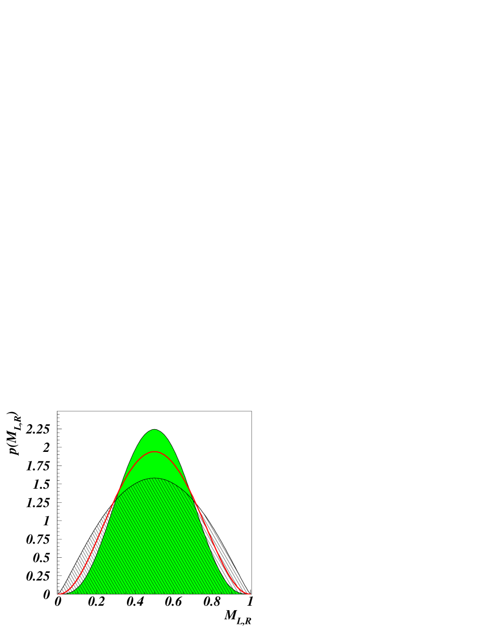
FIG. 1.: Schematic summary of the experimental findings with respect to the scale-invariant $L/R$-multiplier distributions: (thick solid line) unconditional distribution $p(M_{L/R}^{(j+1)})=p(M_{L/R}^{(j+1)}|0\leq M_{L/R}^{(j)}\leq 1)$, (grey) distribution $p(M_{L/R}^{(j+1)}|0\leq\underline{M}\leq M_{L/R}^{(j)}\leq\overline{M}\leq 1/2)$ conditioned on a small $L/R$-parent multiplier, and (hatched) distribution $p(M_{L/R}^{(j+1)}|1/2\leq\underline{M}\leq M_{L/R}^{(j)}\leq\overline{M}\leq 1)$ conditioned on a large $L/R$-parent multiplier.

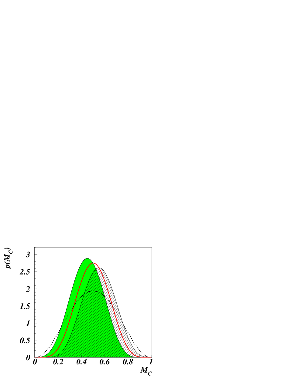
FIG. 2.: Schematic summary of the experimental findings with respect to the scale-invariant centred multiplier distributions: (thick solid line) unconditional distribution $p(M_{C}^{(j+1)})=p(M_{C}^{(j+1)}|0\leq M_{C}^{(j)}\leq 1)$, (grey) distribution $p(M_{C}^{(j+1)}|0\leq\underline{M}\leq M_{C}^{(j)}\leq\overline{M}\leq 1/2)$ conditioned on a small $C$-parent multiplier, and (hatched) distribution $p(M_{C}^{(j+1)}|1/2\leq\underline{M}\leq M_{C}^{(j)}\leq\overline{M}\leq 1)$ conditioned on a large $C$-parent multiplier. For comparison, the unconditional $L/R$-multiplier distribution $p(M_{L/R}^{(j+1)})$ of Fig. 1 is also shown as the thick dash-dotted curve.

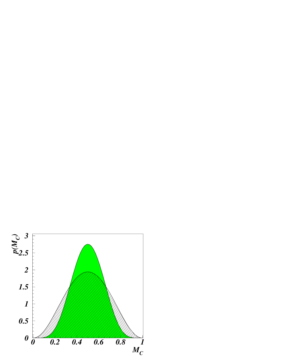
FIG. 3.: Unconditional distribution (8) of centred multipliers $M_{C}^{(j)}$ (grey) following from the $L/R$-splitting function (6) (hatched).

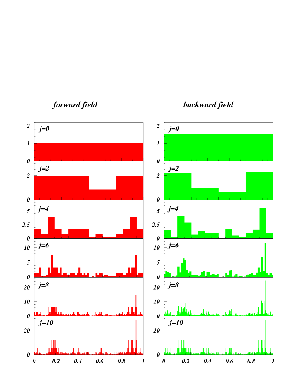
FIG. 4.: Cascade evolution of one energy dissipation field realisation from large to small scales (left column) vs. integrated energy dissipation field from small to large scales (right column). The non-energy flux conserving splitting function (10) has been employed with $\alpha=0.4$ and $J=10$. Only every second scale $j=0,2,\ldots,10$ is shown.

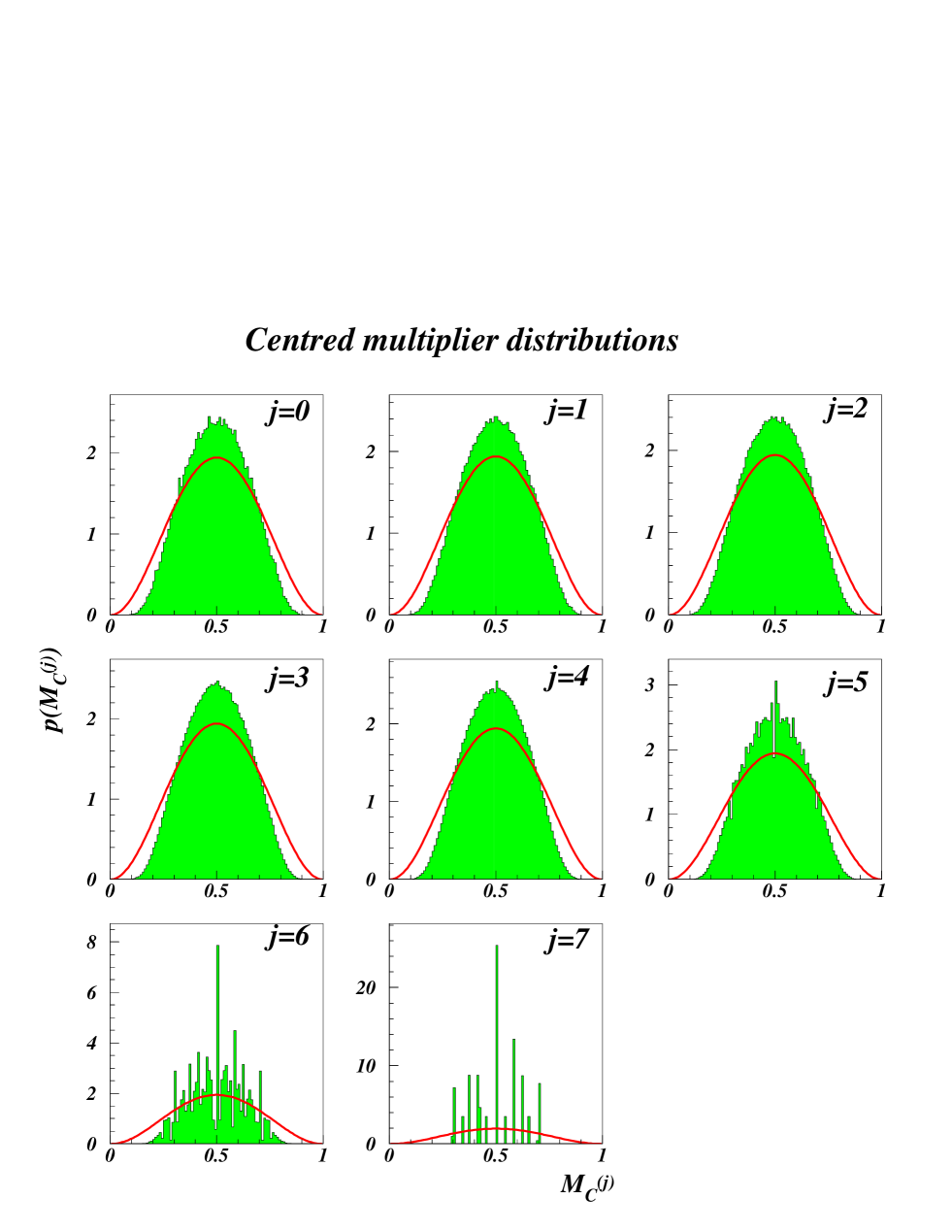
FIG. 5.: Convergence of the (a) left and (b) centred unconditional multiplier distributions $p(M_{L}^{(j)})$ and $p(M_{C}^{(j)})$ of the one-dimensionally observed three-dimensional binomial model (10) to a quasi-continuous limiting form. Parameters are $J=9$, $\alpha=0.4$. For comparison the experimentally deduced Beta-function parametrisation (5) of the left (right) unconditional multiplier distribution with $\beta=3.2$ is shown as a solid line.

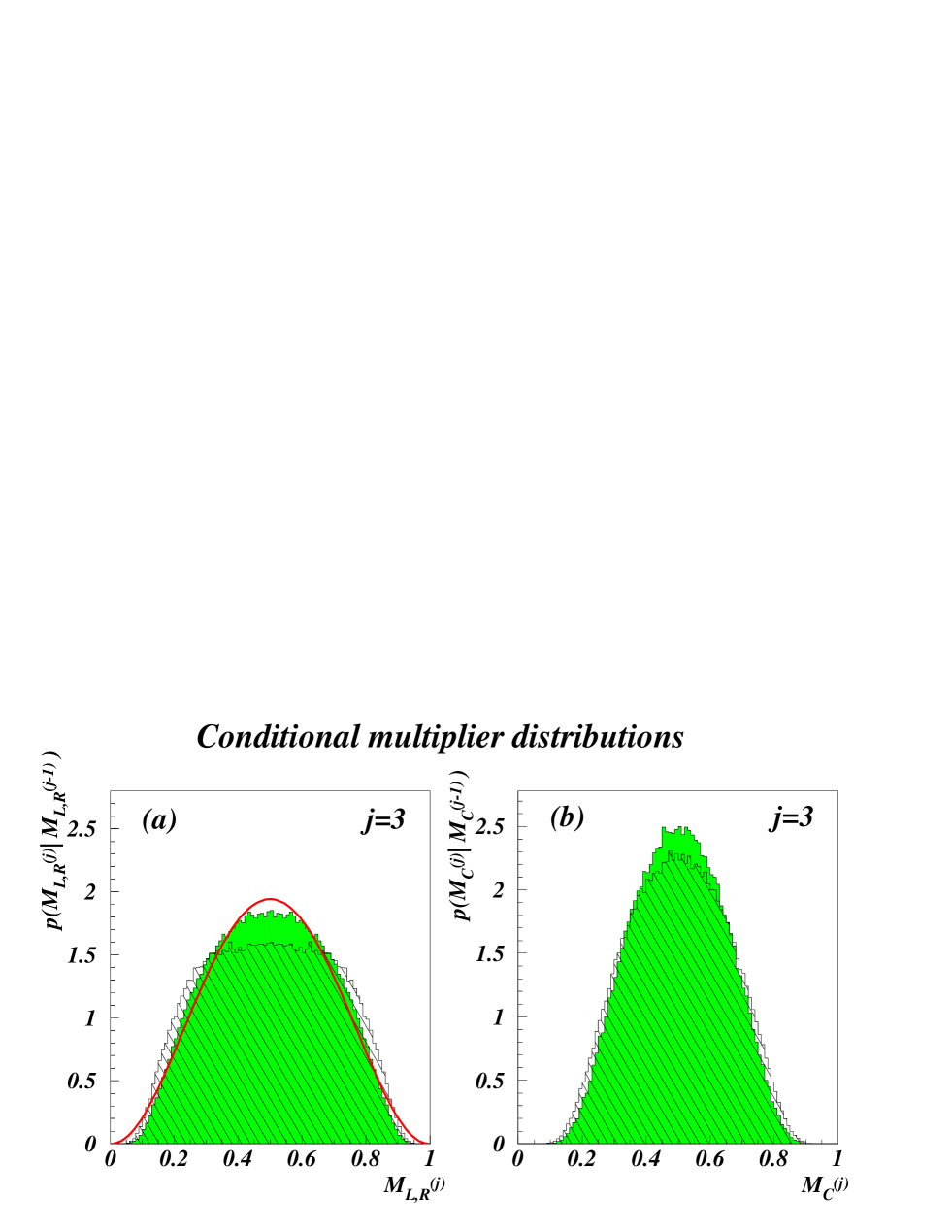
FIG. 6.: Conditional (a) left/right and (b) centred multiplier distributions for scale $j=3$ obtained from the splitting function (10) with $\alpha=0.4$ and $J=9$. (a) $p(M_{L/R}^{(j)}|\underline{M}\leq M_{L/R}^{(j-1)}\leq\overline{M})$ for $\underline{M}=0.2$, $\overline{M}=0.4$ (grey) and $\underline{M}=0.6$, $\overline{M}=0.8$ (hatched); (b) $p(M_{C}^{(j)}|\underline{M}\leq M_{C}^{(j-1)}\leq\overline{M})$ for $\underline{M}=0$, $\overline{M}=0.5$ (grey) and $\underline{M}=0.5$, $\overline{M}=1$ (hatched). For comparison the experimentally deduced Beta-function parametrisation (5) of the left (right) unconditional multiplier distribution with $\beta=3.2$ is shown as a solid curve in (a).

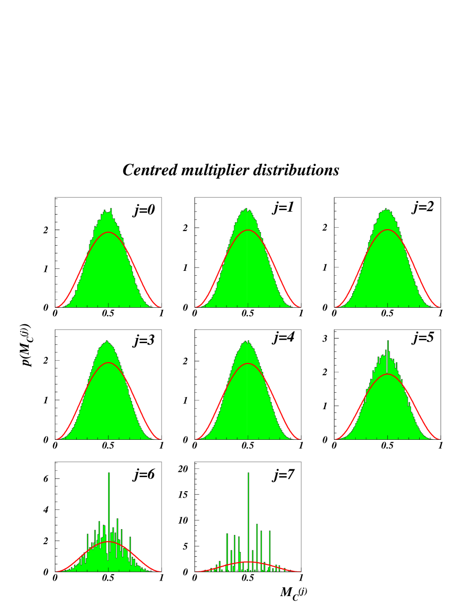
FIG. 7.: Same as Fig. 5, but now after restoration of translational invariance.

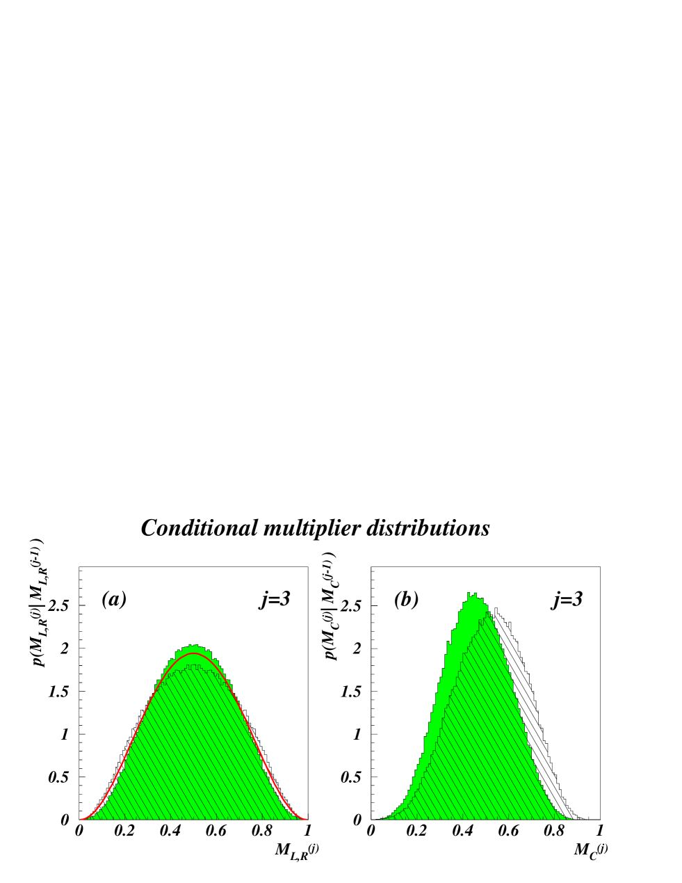
FIG. 8.: Same as Fig. 6, but now after restoration of translational invariance.

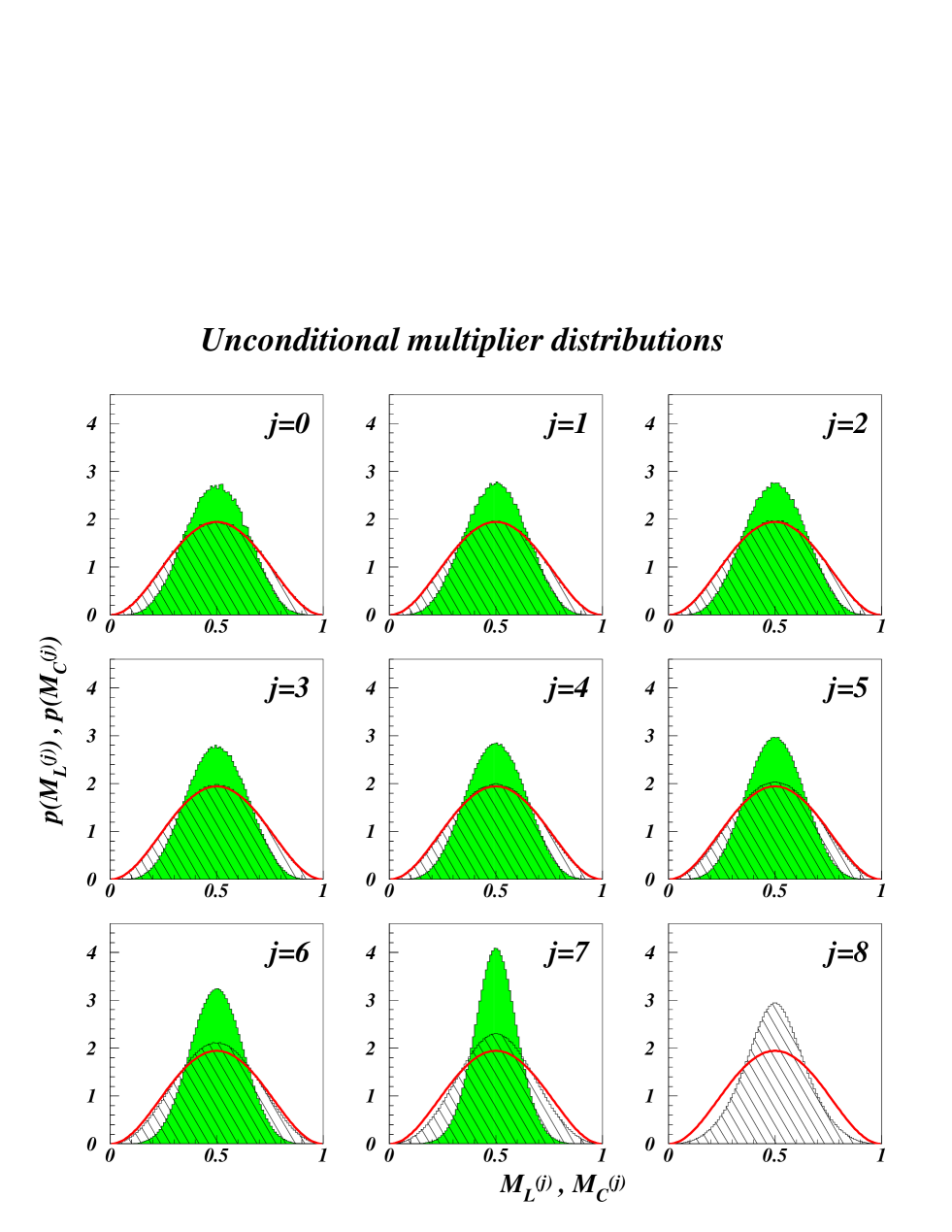
FIG. 9.: Convergence of the left (hatched) and central (grey) unconditional multiplier distributions $p(M_{L}^{(j)})$ and $p(M_{C}^{(j)})$ of the Beta-distribution cascade model (14) to respective limiting forms. Parameters are $J=9$, $\beta=3.2$. For comparison the experimentally deduced Beta-function parametrisation (5) of the left (right) unconditional multiplier distribution with $\beta=3.2$ is shown as a solid line.

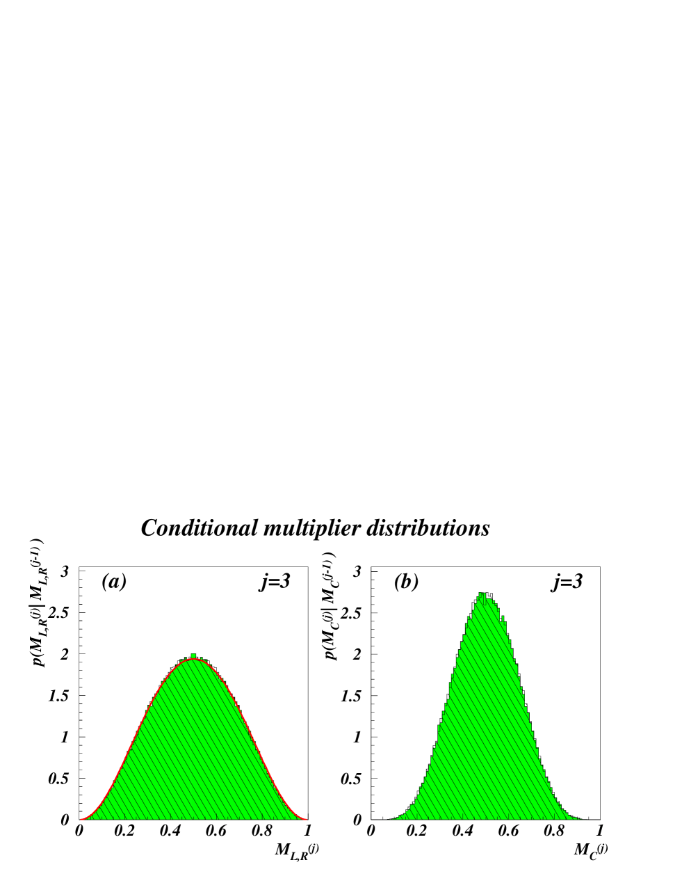
FIG. 10.: Conditional left (a) and centred (b) multiplier distributions for scale $j=3$ obtained from the splitting function (14) with $\beta=3.2$ and $J=9$. (a) $p(M_{L/R}^{(j)}|\underline{M}\leq M_{L/R}^{(j-1)}\leq\overline{M})$ for $\underline{M}=0.2$, $\overline{M}=0.4$ (grey) and $\underline{M}=0.6$, $\overline{M}=0.8$ (hatched); (b) $p(M_{C}^{(j)}|\underline{M}\leq M_{C}^{(j-1)}\leq\overline{M})$ for $\underline{M}=0$, $\overline{M}=0.5$ (grey) and $\underline{M}=0.5$, $\overline{M}=1$ (hatched). For comparison the experimentally deduced Beta-function parametrisation (5) of the left (right) unconditional multiplier distribution with $\beta=3.2$ is shown as a solid curve in (a).

FIG. 11.: Weight curdling over two intermediate cascade steps.

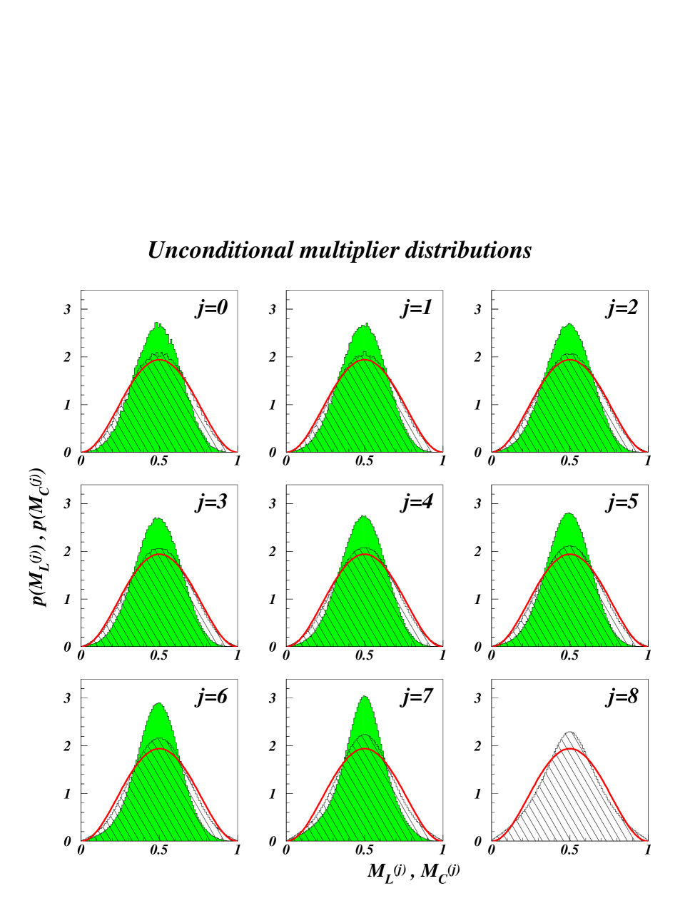
FIG. 12.: Same as Fig. 9, but now after restoration of translational invariance.

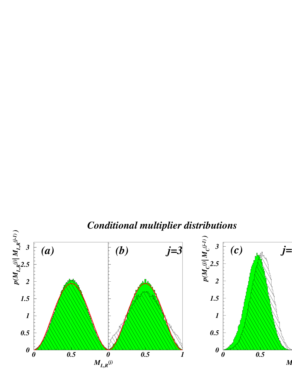
FIG. 13.: Conditional left (a,b) and centred (c) multiplier distributions for scale $j=3$ obtained from the splitting function (14) with $\beta=3.2$ and $J=9$ after restoration of translational invariance. (a) $p(M_{L/R}^{(j)}|\underline{M}\leq M_{L/R}^{(j-1)}\leq\overline{M})$ for $\underline{M}=0.2$, $\overline{M}=0.4$ (grey) and $\underline{M}=0.6$, $\overline{M}=0.8$ (hatched); (b) $p(M_{L/R}^{(j)}|\underline{M}\leq M_{L/R}^{(j-1)}\leq\overline{M})$ for $\underline{M}=0$, $\overline{M}=0.2$ (grey) and $\underline{M}=0.8$, $\overline{M}=1$ (hatched); (c) $p(M_{C}^{(j)}|\underline{M}\leq M_{C}^{(j-1)}\leq\overline{M})$ for $\underline{M}=0$, $\overline{M}=0.5$ (grey) and $\underline{M}=0.5$, $\overline{M}=1$ (hatched). For comparison the experimentally deduced Beta-function parametrisation (5) of the left (right) unconditional multiplier distribution with $\beta=3.2$ is shown as a solid curve in (a,b).

FIG. 14.: Asymmetric weight distributions: (a) asymmetric binomial (30) with $\alpha_{1}=0.5$, $\alpha_{2}=0.3$, (b) asymmetric binomial (30) with $\alpha_{1}=0.3$, $\alpha_{2}=0.65$, (c) log-normal (31) with $\sigma^{2}=0.45$, (d) log-Poisson (32) with $c_{1}=3c_{2}=2$.

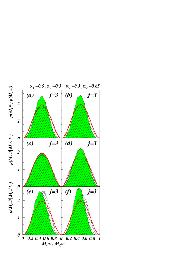
FIG. 15.: Various multiplier distributions resulting from the asymmetric binomial model after restoration of translational invariance. Left column is for model parameters $\alpha_{1}=0.5$, $\alpha_{2}=0.3$, $J=9$, and right column is for $\alpha_{1}=0.3$, $\alpha_{2}=0.65$, $J=9$. First line: unconditional left and centred multiplier distributions $p(M_{L})$ and $p(M_{C})$ at $j=3$; second line: conditional left/right multiplier distribution $p(M_{L/R}^{(j)}|\underline{M}\leq M_{L/R}^{(j-1)}\leq\overline{M})$ for $\underline{M}=0.2$, $\overline{M}=0.4$ (grey) and $\underline{M}=0.6$, $\overline{M}=0.8$ (hatched) at $j=3$; third line: conditional centred multiplier distribution $p(M_{C}^{(j)}|\underline{M}\leq M_{C}^{(j-1)}\leq\overline{M})$ for $\underline{M}=0$, $\overline{M}=0.5$ (grey) and $\underline{M}=0.5$, $\overline{M}=1$ (hatched) at $j=3$. For comparison the experimentally deduced Beta-function parametrisation (5) of the left (right) unconditional multiplier distribution with $\beta=3.2$ is shown as a solid curve in each plot.

FIG. 16.: Various multiplier distributions resulting from the log-normal-model after restoration of translational invariance; parameters are $\sigma^{2}=0.45$, $J=9$. (a) unconditional left and centred multiplier distributions $p(M_{L})$ and $p(M_{C})$ at $j=3$; (b) conditional left/right multiplier distribution $p(M_{L/R}^{(j)}|\underline{M}\leq M_{L/R}^{(j-1)}\leq\overline{M})$ for $\underline{M}=0.2$, $\overline{M}=0.4$ (grey) and $\underline{M}=0.6$, $\overline{M}=0.8$ (hatched) at $j=3$; (c) conditional centred multiplier distribution $p(M_{C}^{(j)}|\underline{M}\leq M_{C}^{(j-1)}\leq\overline{M})$ for $\underline{M}=0$, $\overline{M}=0.5$ (grey) and $\underline{M}=0.5$, $\overline{M}=1$ (hatched) at $j=3$. For comparison the experimentally deduced Beta-function parametrisation (5) of the left (right) unconditional multiplier distribution with $\beta=3.2$ is shown as a solid curve in each plot.

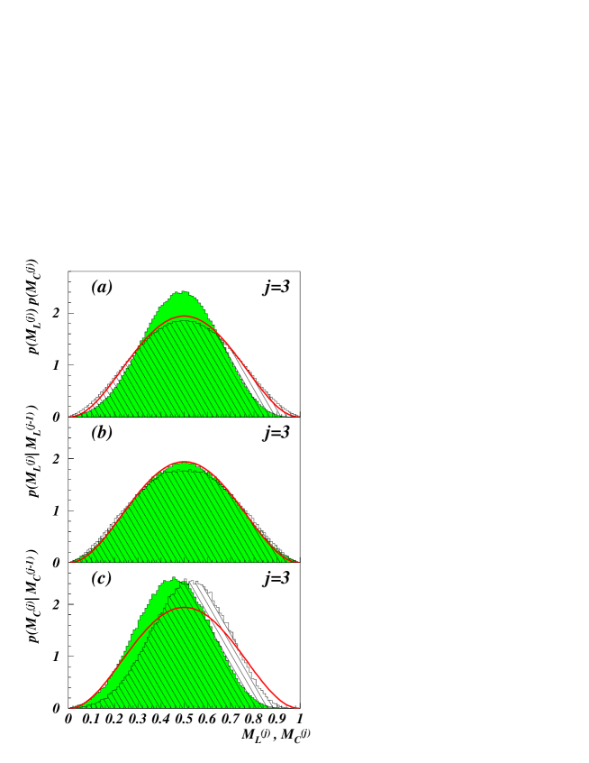
FIG. 17.: Various multiplier distributions resulting from the log-Poisson-model after restoration of translational invariance; parameters are $c_{1}=3c_{2}=2$, $J=9$. (a) unconditional left and centred multiplier distributions $p(M_{L})$ and $p(M_{C})$ at $j=3$; (b) conditional left/right multiplier distribution $p(M_{L/R}^{(j)}|\underline{M}\leq M_{L/R}^{(j-1)}\leq\overline{M})$ for $\underline{M}=0.2$, $\overline{M}=0.4$ (grey) and $\underline{M}=0.6$, $\overline{M}=0.8$ (hatched) at $j=3$; (c) conditional centred multiplier distribution $p(M_{C}^{(j)}|\underline{M}\leq M_{C}^{(j-1)}\leq\overline{M})$ for $\underline{M}=0$, $\overline{M}=0.5$ (grey) and $\underline{M}=0.5$, $\overline{M}=1$ (hatched) at $j=3$. For comparison the experimentally deduced Beta-function parametrisation (5) of the left (right) unconditional multiplier distribution with $\beta=3.2$ is shown as a solid curve in each plot.