On the strong anomalous diffusion

Abstract

The superdiffusion behavior, i.e. $<x^{2}(t)>\sim t^{2\nu}$, with $\nu>1/2$, in general is not completely characherized by a unique exponent. We study some systems exhibiting strong anomalous diffusion, i.e. $<|x(t)|^{q}>\sim t^{q\nu(q)}$ where $\nu(2)>1/2$ and $q\nu(q)$ is not a linear function of $q$. This feature is different from the weak superdiffusion regime, i.e. $\nu(q)=const>1/2$, as in random shear flows.

The strong anomalous diffusion can be generated by nontrivial chaotic dynamics, e.g. Lagrangian motion in $2d$ time-dependent incompressible velocity fields, $2d$ symplectic maps and $1d$ intermittent maps. Typically the function $q\nu(q)$ is piecewise linear. This corresponds to two mechanisms: a weak anomalous diffusion for the typical events and a ballistic transport for the rare excursions.

In order to have strong anomalous diffusion one needs a violation of the hypothesis of the central limit theorem, this happens only in a very narrow region of the control parameters space.

In the presence of the strong anomalous diffusion one does not have a unique exponent and therefore one has the failure of the usual scaling of the probability distribution, i.e. $P(x,t)=t^{-\nu}F(x/t^{\nu})$. This implies that the effective equation at large scale and long time for $P(x,t)$, cannot obey neither the usual Fick equation nor other linear equations involving temporal and/or spatial fractional derivatives.

PACS number(s): 05.45.+b, 05.60.+w;

1 Introduction

The transport of mass or heat from particles passively advected by a given velocity field is a problem of considerable practical and theoretical interest. The coupling between advection and molecular diffusitivy results in a great variety of different fields, as geophysics, chemical engineering and disordered media [1, 2]. One can have highly nontrivial behavior even in the presence of simple laminar velocity fields, e.g. very large diffusion coefficients due to the combined effects of the molecular diffusitivy and some features of the velocity fields [1, 3].

Taking into account the molecular diffusion, the Lagrangian motion of a test particle is described by the Langevin equation :

$$\dot{\mbox{\boldmath$x$}}={\mbox{\boldmath$u$}}({\mbox{\boldmath$x$}},t)+{\mbox{\boldmath$\xi$}}$$ (1)

where ${\mbox{\boldmath$u$}}({\mbox{\boldmath$x$}},t)$ is the Eulerian velocity field at the position $x$ and the time $t$, and $\xi$ is a Gaussian white noise with zero mean and correlation function

$$\langle\xi_{i}(t)\xi_{j}(t^{\prime})\rangle=2D_{0}\delta_{ij}\;\delta(t-t^{\prime}),$$ (2)

the coefficient $D_{0}$ being the molecular diffusivity. If $\Theta$ is the density of tracers, the Fokker–Planck equation associated to (1) is

$$\partial_{t}\Theta+{\mbox{\boldmath$\partial$}}({\mbox{\boldmath$u$}}\;\Theta)=D_{0}\partial^{2}\Theta.$$ (3)

For times much larger than the typical time of $u$, the large-scale density field $\langle\theta\rangle$ (i.e. the field $\theta$ averaged over a volume of linear dimension much larger than the typical length of the velocity field $u$) obeys a standard diffusion Fick equation:

$$\partial_{t}\langle\Theta\rangle=D^{E}_{ij}\partial^{2}_{x_{i}x_{j}}\langle\Theta\rangle\;\;\;\;\;\;i,j=1,\ldots,d.$$ (4)

All the (often nontrivial) effects due to the presence of the velocity field are in the eddy diffusion coefficient $D^{E}_{ij}$. Of course if the Eq. (4) holds then one has $\langle(x(t)-x(0))^{2}\rangle\simeq 2\;D^{E}_{11}\;t$. In practice at large time the test particle behaves as a Brownian particle.

The above scenario is the typical one. Nevertheless there exist cases where anomalous diffusion is observed, i.e. $\langle(x(t)-x(0))^{2}\rangle\sim t^{2\nu}$ with $\nu\neq 1/2$. The case when $\nu<1/2$ corresponds to subdiffusion while for $\nu>1/2$ one has superdiffusion. Trapping is the basic mechanism leading to subdiffusion and it occurs only in compressible fields. A remarkable example of subdiffusion, $\langle(x(t)-x(0))^{2}\rangle\sim[\ln(t)]^{4}$ is the random walk in $1d$ random potential [4].

If the velocity field is incompressible and the molecular diffusivity is non zero, either standard diffusion or superdiffusion takes place.

In the last two decades many authors have studied systems with anomalous (non Gaussian) diffusion. It is practically impossible to cite the huge literature. We just mention, among the many, the contribution of Geisel and coworkers [5] for the $1d$ intermittent maps, Ishizaki et al [6] for the symplectic maps, Zaslavky et al [7] for the lagragian motion in q-flows [8, 9], Majda & Avellaneda [10] for the random shear flows, the experimental study of Solomon at al. [11] on the superdiffusion in an anular tank, the symbolic dynamics approach of Misguich et al. [12] for the subdiffusive behavior in a stochastic layer and the anomalous diffusion of magnetic lines in the $3d$ turbulence by Zimbardo et al. [13].

The aim of this paper is a detailed study of the anomalous diffusion in simple velocity fields and discrete time dynamical systems. In particular we shall show that strong anomalous diffusion may occur, i.e.

$$\langle(x(t)-x(0))^{q}\rangle\sim t^{q\,\nu(q)}$$ (5)

where $\nu(q)$ is non-constant. In this case the probability distribution $P(x,t)$ cannot be described in term of a unique scaling exponent, as in the Lévy flight [14] or in the random shear flow.

Section 2 is devoted to a brief review of the known mechanisms for anomalous diffusion. In Sec. 3 we report detailed numerical results for the anomalous diffusion mechanism in $2d$ time-dependent incompressible velocity field, in the standard map (which can be considered a discrete time version of the Lagrangian motion in a $2d$ time periodic incompressible velocity field), and in an intermittent $1d$ map. In Sec. 4 the reader can find some conjectures and discussions.

2 A brief review on some aspects of the anomalous diffusion

Anomalous diffusion occurs when some, or all, of the hypothesis of the central limit theorem break down. Practically, the system has to violate at least one of the two following conditions :

• finite variance of the velocity;

• fast enough decay of the auto-correlation function of Lagrangian velocities.

This is, of course, an elementary remark. Nevertheless, in our opinion, a detailed discussion of this point can be useful. In the present paper we use the term anomalous diffusion to indicate a non standard diffusion in the asymptotic limit of very long time. Sometimes in the literature the term anomalous is used also for long (but non asymptotic) transient behavior. This transient anomalous behavior can have practical relevance, e.g. in geophysics. We do not discuss this point in details. Let us recall some well established results on the relation between diffusion phenomena and correlation function. It is easy to obtain the following formula :

$$\langle\left(x_{i}(t)-x_{i}(0)\right)^{2}\rangle=\int_{0}^{t}dt_{1}\int_{0}^{t}dt_{2}\langle v_{i}({\mbox{\boldmath$x$}}(t_{1}))\;v_{i}({\mbox{\boldmath$x$}}(t_{2}))\rangle\simeq 2\;t\;\int_{0}^{t}d\tau\;C_{ii}(\tau)$$ (6)

where $C_{ij}(\tau)$ is the correlation function of the Lagrangian velocity, namely ${\mbox{\boldmath$v$}}=\dot{\mbox{\boldmath$x$}}$,

$$C_{ij}(\tau)=\langle\;v_{i}({\mbox{\boldmath$x$}}(\tau))\;v_{j}({\mbox{\boldmath$x$}}(0))\;\rangle.$$ (7)

Eq. (6) is the so-called Taylor relation [15] for a test particle evolving according to the Langevin equation (1).

For test particles whose dynamics is described by a map (discrete time),

$${\mbox{\boldmath$x$}}(n+1)={\mbox{\boldmath$F$}}({\mbox{\boldmath$x$}}(n)),$$ (8)

the Taylor formula (6) is still valid with the obvious changes : ${\mbox{\boldmath$v$}}({\mbox{\boldmath$x$}}(t))\mapsto{\mbox{\boldmath$F$}}({\mbox{\boldmath$x$}}(n))-{\mbox{\boldmath$x$}}(n)$ and $\int_{0}^{t}C_{ii}(\tau)\mapsto C_{ii}(0)/2+\sum_{j=1}^{n}C_{ii}(j)$. If both $\langle v^{2}\rangle<\infty$ and $\int_{0}^{t}d\tau\;C_{ii}(\tau)<\infty$ then one has standard diffusion and the effective diffusion coefficients are

$$D^{E}_{ii}=\lim_{t\rightarrow\infty}\frac{1}{2\;t}\langle\left(x_{i}(t)-x_{i}(0)\right)^{2}\rangle=\int_{0}^{\infty}\;d\tau\;C_{ii}(\tau)$$ (9)

From the above remarks it stems that anomalous diffusion occurs only in two circumstances:

• $\langle v^{2}\rangle=\infty$

• $\langle v^{2}\rangle<\infty$ and $\int_{0}^{t}d\tau\;C_{ii}(\tau)=\infty$, i.e. $C_{ii}(\tau)\sim\tau^{-\beta}$ with $\beta>1$, that means very strong correlations.

2.1 Simple systems exhibiting anomalous diffusion

The Lévy flight [14] belongs to the first case. Let us briefly discuss it for discrete one dimensional systems. The position $x(t+1)$ at the time $t+1$ is obtained from $x(t)$ as follows:

$$x(t+1)=x(t)+U(t),$$ (10)

where $U(t)$’s are independent variables identically distributed according to a $\alpha$–Lévy–stable distribution, $P_{\alpha}(U)$, with the following well-known properties :

$$\int\;dUe^{ikU}P_{\alpha}(U)\propto e^{-c\mid k\mid^{\alpha}}\;\;\;\;{\rm and}\;\;\;\;P_{\alpha}(U)\sim U^{-(1+\alpha)}\;\;\;\;{\rm for}\;\;\;\;\mid U\mid\gg 1$$ (11)

with $0<\alpha\leq 2$. An easy computation gives

$$\langle x(t)^{q}\rangle=\left\{\begin{array}[]{cc}C_{q}\;t^{q/\alpha}&q<\alpha\\ \infty&q\geq\alpha.\end{array}\right.$$ (12)

Note that $\langle x^{2}\rangle=\infty$ for any $\alpha<2$, nevertheless one can consider the Lévy flight as a sort of anomalous diffusion in the sense that $x\sim t^{1/\alpha}\gg t^{1/2}$.

In spite of the relevance of the $\alpha$–Lévy–stable distribution in probability theory, the Lévy flight model, in our opinion, has a rather weak importance for physical systems. This is due to the very unrealistic property of infinite variance.

An elegant way to overcome the above trouble is the introduction of a stochastic model, called Lévy walk [16], corresponding to (10) but now $U(t)$ is a random variable with nontrivial correlations. The velocity $U(t)$ can assume the values $\pm u_{0}$ and it maintains its value for a duration $T$ which is a random variable with probability density $\psi(T)$. Practically, the particle moves with constant velocity for a certain time after which it changes direction and so on. In the Lévy walk the origin of the possible anomaly is transferred to the correlation function of the Lagrangian velocity. Actually, taking

$$\psi(T)\sim T^{-(\alpha+1)},$$ (13)

one has standard diffusion if $\alpha>2$ while for $\alpha<2$ one has anomalous (super) diffusion :

$$\langle x(t)^{2}\rangle\sim t^{2\nu}\;\;\;\;\;\nu=\left\{\begin{array}[]{cc}1/2&\alpha>2\\ (3-\alpha)/2&1<\alpha<2\\ 1&\alpha<1.\end{array}\right.$$ (14)

Sometimes in the literature the Lévy walk is (erroneously) called Lévy flight.

2.2 Nontrivial anomalous diffusion

From the above considerations one realizes that it is not particularly difficult to build up ad hoc probabilistic models exhibiting anomalous diffusion. On the contrary it is much more difficult and much more interesting the understanding of the anomalous diffusion in nontrivial systems like the transport in incompressible velocity fields or deterministic maps, where the explicit probabilistic aspect (given for example by an external noise related to the molecular diffusivity) cannot play a relevant role.

Avellaneda and Majda [17], (see also Avellaneda & Vergassola [18] for the generalization to the time dependent case), obtained a very important and general result about the diffusion in an incompressible velocity field ${\mbox{\boldmath$u$}}({\mbox{\boldmath$x$}})$. If the molecular diffusivity $D_{0}$ is non zero and the infrared contribution to the velocity field are weak enough, namely

$$\int d{\mbox{\boldmath$k$}}\;\frac{\langle\mid\hat{{\mbox{\boldmath$u$}}}({\mbox{\boldmath$k$}})\mid^{2}\rangle}{k^{2}}<\infty$$ (15)

where $\langle\;\cdot\;\rangle$ indicates the time average and $\hat{{\mbox{\boldmath$u$}}}$ represents the Fourier transform of the velocity field, then one has standard diffusion, i.e. the diffusion coefficients $D_{ii}$’s in (9) are finite. Therefore there exist two possible origins for the superdiffusion

• $D_{0}>0$ and, in order to violate the (15), the velocity field with very long spatial correlation;

• $D_{0}=0$ and strong correlation between ${\mbox{\boldmath$u$}}({\mbox{\boldmath$x$}}(t))$ and ${\mbox{\boldmath$u$}}({\mbox{\boldmath$x$}}(t+\tau))$ at large $\tau$.

For the sake of completeness we briefly remind one of the few nontrivial systems for which the presence of anomalous diffusion can be proven in a rigorous way.

Consider a $2d$ random shear flow :

$${\mbox{\boldmath$u$}}=\left(u(y)\;,\;0\right)$$ (16)

where $u(y)$ is a random function such that

$$u(y)=\int_{-\infty}^{\infty}dk\;e^{iky}\;\hat{u}(k)\;\;\;\;\;\;\;\langle\hat{u}(k)\;\hat{u}(k^{\prime})\rangle=S(k)\;\delta(k-k^{\prime}),$$ (17)

$S(k)$ is the spectrum and the average $\langle\;\cdot\;\rangle$ is taken over the field realizations. Matheron & De Marsily [8] showed that the anomalous diffusion in the $x$-direction occurs if

$$\int dk\;\frac{S(k)}{k^{2}}=\infty.$$

On the contrary, if this integral is finite one has standard diffusion and

$$D^{E}_{11}=D_{0}+\frac{1}{D_{0}}\int_{0}^{\infty}dk\;\frac{S(k)}{k^{2}}.$$ (18)

Eq. (18) is a well-known exact result already obtained by Zeldovich [19]. For the sake of simplicity we consider the case

$$S(k)\sim k^{\gamma}\;\;\;\;\;k\mapsto 0.$$ (19)

If $\gamma>1$ then one has standard diffusion. On the contrary, if $-1\leq\gamma\leq 1$ one has a superdiffusion, namely

$$\langle\;\mid x(t)-x(0)\mid^{2}\;\rangle\sim t^{2\nu}\;\;\;\;\;\;\nu=\frac{3-\gamma}{4}\geq\frac{1}{2}.$$ (20)

The condition $\int dk\;S(k)\;k^{-2}=\infty$ for the anomalous diffusion can be understood by means of the following simple physical argument. Note that $\int dk\;S(k)\;k^{-2}\sim\langle u^{2}\rangle\;L^{2}$ where $L$ is the typical length of the function $u(y)$, i.e. the typical distance between two sequent zeros of $u(y)$. If $\langle u^{2}\rangle<\infty$ and $\int dk\;S(k)\;k^{-2}<\infty$ the diffusion process is basically similar to that one characterized by a velocity field given by a sequence of strips of size $L$ and velocity $\pm\sqrt{\langle u^{2}\rangle}$ and therefore the (18) is nothing but the transversal Taylor diffusion [20] in channels. The origin of the anomalous diffusion in this case is due to the fact that a test particle travels in a given direction for a very long time before it changes direction and so on. In some sense the Lagrangian motion in the random shear flow for $-1\leq\gamma\leq 1$ is a nontrivial realization of a Lévy walk. The generalization to the $3d$ case ${\mbox{\boldmath$u$}}=\left(u(y,z),0,0\right)$ is straightforward.

Another nontrivial system where the presence of anomalous diffusion has been rigorously proven is the Kraichnan’s passive scalar model [21], where the velocity advecting the scalar field, is rapidly varying in time. For such a model, generally, the distance between pairs of particles tends to increase with the time elapsed but, occasionally, particles may come very close and stay so; this is the source of the anomalies in the scaling [22] [23].

If the inequality (15) holds then in order to have anomalous diffusion one needs $D_{0}=0$ and a correlation function $C_{ii}(\tau)$ going to zero not too fast. These conditions are satisfied, e.g., in time periodic velocity fields whose Lagrangian phase space has a complicated self-similar structure of island and cantori [7]. In this case superdiffusion is essentially due to the almost trapping of the trajectories for arbitrarily long time, close to the cantori which are organized in complicated self-similar structures.

In addition, there exist a strong numerical evidence (and sometimes also theoretical arguments) for superdiffusion in $1$-d intermittent maps as well as in the standard map, which is a $2$-d symplectic map and therefore it can be considered as the Poincaré map of a Lagrangian motion in a time periodic velocity field.

2.3 About the meaning of anomalous

Up to now we used the term anomalous as synonymous of non-Gaussian. Let us consider now in more detail the cases with superdiffusion. There are two possibilities :

• weak anomalous diffusion when

  $$\langle\mid x(t)-x(0)\mid^{q}\rangle\sim t^{q\nu}\;\;\;\;\forall q>0\;\;{\rm and}\;\;\nu>\frac{1}{2}$$ (21)

• strong anomalous diffusion when

  $$\langle\mid x(t)-x(0)\mid^{q}\rangle\sim t^{q\,\nu(q)}\;\;\;\;\nu(q)\neq cost\;\;\;\nu(2)>\frac{1}{2}$$ (22)

  where $\nu(q)$ is a nondecreasing function of $q$.

In the weak anomalous diffusion one has for the probability distribution $P(\Delta x,t)$ of $\Delta x=x(t)-x(0)$ at time $t$, the following expression :

$$P(\Delta x,t)=t^{-\nu}F(\Delta x\;t^{-\nu})$$ (23)

where in general the function $F$ is different from the Gaussian one. The random shear flow is an example of the weak anomalous diffusion [9].

Bouchaud at al. [24] have shown that in the case of the random shear flow (16)-(18) with $\gamma=0$

$$F(a)\sim e^{-c\mid a\mid^{4/3}}\;\;\;{\rm for}\;\;\mid a\mid\gg 1.$$ (24)

There are very few numerical studies on the strong anomalous diffusion. Let us mention the work of Sneppen & Jensen [25] on the motion of particles passively advected by the dynamical membranes (the authors use the term multidiffusion) and an $1$-d intermittent map studied by Pikovsky [26].

Of course the strong anomalous diffusion is not compatible with the simple scaling (23). Obviously in the presence of anomalous diffusion $P(x,t)$ cannot obey to the usual Fickian diffusion Eq. (8). Therefore, a quite natural problem is to find the effective evolution equation for $P(x,t)$ at large $t$. The answer to this question up to now as far as we know, is not well understood in the general case.

For the Lévy flight one can naively write

$$\partial_{t}P=-c\;(-\partial^{2})^{\alpha/2}\;P.$$ (25)

The above equation can be considered the proper one for the Lévy flight in the sense that starting at $t=0$ with $P(x,0)=\delta(x)$ at any $t>0$ the probability $P(x,t)$ is given by th $\alpha$-stable Lévy function. Of course, if $\alpha=2$ one has the usual Fick equation and the Gaussian shape for $P(x,t)$. For the more complicated anomalous diffusion there are many proposal in terms of fractional time, and/or spatial, derivatives. We do not enter in a detailed discussion of these works, the interested readers can see [27].

3 Numerical results

In this section we report detailed numerical results for anomalous diffusion in $2$-d time dependent velocity fields and maps.

3.1 Strong anomalous diffusion in a simple flow mimicking the Rayleigh–Bénard convection

We investigate here anomalous diffusion in a simple model mimicking the Rayleigh–Bénard convection [28, 29]. Two-dimensional convection with rigid boundary conditions is described by the following stream function:

$$\psi(x,y,t)=\psi_{0}\sin(x+B\sin\omega t)\sin y\;\;\;,$$ (26)

where the periodicity of the cell is $L\equiv 2\pi$, and the even oscillatory instability [30] is accounted for by the term $B\sin\omega t$, representing the lateral oscillation of the rolls. The capability of the simple flow (26) to capture the essential features of the convection problem is discussed in Ref. [29].

It is worth noting that, at fixed $B$, the only relevant parameter controlling the diffusion process in the flow (26) is $\epsilon\equiv\omega L^{2}/\psi_{0}$, i.e., the ratio between the lateral roll oscillation frequency and the characteristic frequency of the passive scalar motion. Different regimes take place for different values of $\epsilon$. The two limiting cases $\epsilon\ll 1$ and $\epsilon\gg 1$ have been investigated in Ref. [31]. The regime $\epsilon\sim 1$ has recently been studied in Ref. [32], in particular the synchronization between the lateral roll oscillation frequency (of the order of $\omega$) and the characteristic frequencies of the scalar field motion (of the order of $\psi_{0}/L^{2}$) has been investigated. This mechanism leads to enhanced diffusion.

We briefly recall the main results of Ref. [32]. It has been found that the synchronization between the circulation in the cells and their global oscillation is a very efficient way of jumping from cell to cell. This mechanism, similar to stochastic resonance [33, 34], makes the effective diffusivity as a function of the frequency $\omega$ very structured. In the limit where the molecular diffusion vanishes, anomalous superdiffusion takes place for narrow windows of values of $\omega$ around the peaks.

In Fig. 1 the $x$-component, $D^{E}_{11}$, of the eddy diffusivity versus the frequency $\omega L^{2}/\psi_{0}$ is shown for different values of $D_{0}/\psi_{0}$.

Figure 1: The turbulent diffusivity $D^{E}_{11}/\psi_{0}$ vs the frequency $\omega L^{2}/\psi_{0}$ for different values of the molecular diffusivity $D_{0}/\psi_{0}$. $D_{0}/\psi_{0}=3\times 10^{-3}$ (dotted curve); $D_{0}/\psi_{0}=1\times 10^{-3}$(broken curve); $D_{0}/\psi_{0}=5\times 10^{-4}$ (full curve).

We anticipate that anomalous diffusion in the strong sense (according to the definition given in Sec. 2.2) takes place, making highly nontrivial the diffusion process only around the values of $\omega$ corresponding to the peaks of enhanced diffusion. Specifically, let us focus our attention on the anomalous regime occurring for $D_{0}=0$ and $\omega L^{2}/\psi_{0}\simeq 1.1$. We have then integrated the Eq. (11) with $D_{0}=0$ and $u$ obtained from the flow (26), using a second-order Runge-Kutta scheme. In the following, averages are over different realizations and performed by uniformly distributing $10^{6}$ particles in the basic periodic cell. The system evolution is computed up to times of the order of $10^{4}\;L^{2}/\psi_{0}$.

In order to investigate the anomalous diffusion in the strong sense, a measure of $\langle[x(t)-x(0)]^{q}\rangle$ for different $q$’s has to be made.

Figure 2: The mean-squared displacement vs the time for the flow (26) with $D_{0}=0$, and $\omega=1.1$. Lengths and times are shown in units of $L$ and $L^{2}/\psi_{0}$, respectively. The best-fit (dashed) line corresponds to $2\nu(2)=1.3$.

To that end, we have performed a linear fit of $\ln\langle[x(t)-x(0)]^{q}\rangle$ versus $\ln t$, the slope of which being the exponent $q\,\nu(q)$ in (22). As an example, in Fig. 2 the mean-squared displacement, as a function of the time, has been presented. Superdiffusive transport takes thus place for $\omega=1.1$ in the limit $D_{0}\to 0$, i.e.:

$$\langle[x(t)-x(0)]^{2}\rangle\propto t^{2\nu(2)}\qquad\mbox{with}\qquad\nu(2)>1/2\;\;\;.$$ (27)

The presence of genuine anomalous diffusion is also supported by the behavior of the coefficient $D^{E}_{11}$ as a function of $D_{0}$. As suggested in Ref. [35], in the presence of genuine anomalous diffusion, the effective diffusivity must diverge and it is expected that $D^{E}_{11}\sim D_{0}^{-\beta}$ with $\beta>0$.

Figure 3: The diffusion coefficient $D^{E}_{11}$ as a function of $D_{0}$ for the frequency of the roll oscillation $\omega=1.1$. The diffusivities are reported in units of $\psi_{0}$. The best-fit (dashed) line has the slope $-\beta=-0.18$.

The curve $D^{E}_{11}$ versus $D_{0}$ is shown in Fig. 3. The data are well fitted by a straight line with slope $\beta\simeq 0.18$, confirming the presence of anomalous diffusion at $D_{0}=0$.

Fits similar to that one presented in Fig. 2 have been obtained also for other values of the order $q$, ranging between $0$ and $6$. The results are summarized in Fig. 4,

Figure 4: The measured scaling exponents $q\,\nu(q)$’s (joined by dot-dashed straight lines) of the moments of the displacement $\Delta x$, as a function of the order $q$. The dashed line corresponds to $0.65\;q$ while the dotted line corresponds to $q-1.04$.

where the exponents $q\,\nu(q)$’s are shown as a function of $q$.

Some remarks are in order. The curve, as a whole, displays a nonlinear behavior, the first clue of anomalous diffusion in the strong sense. Two linear regions are actually present: the first one behaves up to $q\sim 2$, the second elsewhere. The two linear regions are associated to two different mechanisms in the diffusion process, as suggested by the following simple considerations. For small $q$’s, i.e. for the core of the probability distribution function $F(\Delta x,t)$, only one exponent $\nu_{1}\equiv\nu(q)\simeq 0.65$ for $q\lesssim 2$ fully characterizes the diffusion process even if anomalous. The typical, i.e. non rare, events obey a (weak) anomalous diffusion process, roughly speaking, one can say that at scale $l$ the characteristic time $\tau(l)$ behaves like

$$\tau(\l)\sim l^{1/\nu_{1}}.$$ (28)

On the other hand, the behavior $q\,\nu(q)\simeq q-1.04$ suggests that the large deviations are essentially associated to ballistic transport

$$\tau(\l)\sim l$$ (29)

basically due to the mechanism of synchronization between the circulation in the cells and their global oscillation.

The character of strong anomalous diffusion, already evident from Fig. 4, is highlighted by the behavior of the probability density function (p.d.f.), $P(\Delta x,t)$, of the displacement $\Delta x=x(t)-x(0)$ at different times t’s. As already pointed out in Sec. 2.3, weak and strong anomalous diffusion can indeed carefully be discriminated by means of the simple scaling law (23), which is not compatible with the strong anomalous diffusion. We have considered three different probability distribution functions for three different times, namely: $P_{1}(\Delta x,t_{1})$, $P_{2}(\Delta x,t_{2})$ and $P_{3}(\Delta x,t_{3})$, with $t_{3}=2t_{2}=4t_{1}$ and $t_{1}$, $t_{2}$ and $t_{3}$ are well inside the scaling regions of the moments of the displacement. In Fig. 5

Figure 5: The normalized probability distribution function $P(\Delta x(t)/\tilde{\sigma})$ vs $\Delta\tilde{x}\equiv\Delta x/\tilde{\sigma}$ for the three times $t_{1}=500$ (circles), $t_{2}=2t_{1}$ (diamond) and $t_{3}=2t_{2}$ (squares). The dashed line represents the Gaussian function, shown for comparison.

the three renormalized probability distribution functions $P(\Delta x(t)/\tilde{\sigma})$, with $\tilde{\sigma}=\exp\langle\ln\mid\Delta x(t)\mid\rangle$, at $t=t_{1}$, $t_{2}$ and $t_{3}$, respectively, are shown.

Some remarks are in order. The first one concerns the tails of the three probability distribution functions which are clearly much higher than those of the Gaussian one. The strong character of the anomalous diffusion can be easily investigated by observing that if the scaling law (23) holds then the three functions rescaled probability distributions at different times have to be superimposed one on the other. As one can see from Fig. 5, this is not the case in our system. In fact, one satisfies (23) but only for small deviations, that means that only the cores of the probability distribution functions obey the above scaling law. This fact is not surprising being a direct consequence of the behavior shown for the scaling exponents $q\,\nu(q)$’s. It is worth noting that the anomalous behavior disappears for a very small changes of the parameters, e.g. for $\omega=1.075$ standard diffusion takes place.

3.2 Standard and anomalous diffusion in the standard map

The standard map is a well-known symplectic map [36], [37], given by:

$$\left\{\begin{array}[]{l}J_{t+1}=J_{t}+\frac{A}{2\,\pi}\sin(2\,\pi\,\theta_{t})\\ \theta_{t+1}=\theta_{t}+J_{t+1}\quad\;\;\;\;{\rm mod}\;1.\end{array}\right.$$ (30)

A short review of its phenomenology follows. For $A=0$ it is integrable

$$\left\{\begin{array}[]{l}J_{t}=J_{0}\quad\forall\,t\\ \theta_{t}=\theta_{0}+t\,J_{0}\quad{\rm mod}\,1;\end{array}\right.$$ (31)

for all rational $J_{0}$ one has periodic motion on resonant tori. As soon as $A>0$ the resonant tori disintegrate in pairs of elliptic and hyperbolic fixed points according to the Poincaré-Birkhoff theorem [36]. In the corresponding regions chaotic motions may occur. Still for small values of $A$ the orbits remain trapped in invariant sets. This is due to the persistence under small perturbation of the nonresonant (KAM) tori where aperiodic motions take place and to the topological constraint imposed by the dimensionality of the system. In two dimensions the chaotic orbits generated by the disintegration of resonant tori are restricted to lie between two bounding KAM curves. Since the latter ones are invariant and the area enclosed by them is conserved by symplecticity the chaotic regions are also invariant and no diffusion can take place [36]

In order to observe diffusive behaviors one must consider values of $A$ large enough so that all KAM tori which connect $\theta=-0.5$ to $\theta=0.5$ disappear. The critical value of $A$ has been numerically determined to be $A_{c}\simeq 0.97$ [38]. For $A>A_{c}$ the phase space can be pictorially described as a chaotic sea where islands of regular motions emerge. Such islands are related to the existence of accelerator modes i.e. stable periodic solutions of (30) specified by:

$$\left\{\begin{array}[]{l}J_{t+p}-J_{t}=l\\ A\sum_{t=1}^{p}\sin(2\,\pi\theta_{t})=2\pi l\end{array}\right.$$ (32)

Each accelerator mode can be labelled with the integer pair $(p,l)$. It is easy to check the stability for $(1,l)$: the symplectic property implies that the Jacobian matrix of (30) computed on a stable solution must give a pair of complex eigenvalues of magnitude one. The condition is satisfied for all $A$ such that:

$$2\,\pi|l|\leq\,A\,\leq 2\,\pi|l|\sqrt{1+\left(\frac{2}{\pi\,l}\right)^{2}}$$ (33)

Expression (33) implies that period one accelerator modes with different $l$ cannot coexist. Furthermore the length of the interval of $A$ values such that $(1,l)$ is stable decreases for large $l$ as:

$$\Delta A\sim\frac{1}{|l|}$$ (34)

If only one stable island exists no sensitive contribution to the diffusion properties of the chaotic orbits is expected. A trajectory that arrives in the neighbourhood of a stable island sticks to it for a finite amount of time before getting away. On average the contribution to the encircling orbit is zero. Typically one observes normal diffusion [39]:

$$\langle[J_{t}-J_{0}]^{2}\rangle\simeq 2\,D\,t\;\;\;\;\;t\gg 1$$ (35)

where the average is over the initial conditions, the diffusion coefficient $D$ can be estimated with a crude random phase approximation as:

$$D\simeq D_{QL}=\frac{1}{2}\langle\left(J_{t+1}-J_{t}\right)^{2}\rangle=\frac{1}{2}\left(\frac{A}{2\,\pi}\right)^{2}\int_{0}^{1}d\theta\,\sin^{2}(2\pi\theta)=\frac{A^{2}}{16\pi^{2}}.$$ (36)

In Fig. 6 the standard diffusion behavior of the exponent $q\,\nu(q)$ as a function of $q$ is shown for $A=3.86$ i.e. in the absence of any stable islands whereas. The same standard diffusion occurs for $A=10.492927$ when one stable island exists [37],[6]. For both the cases standard diffusion occurs.

Figure 6: The diffusion exponent $q\,\nu(q)$ as a function of $q$ for $A=3.86$. The results have been obtained by averaging over $10^{6}$ trajectories with $J_{0}=0$.

The coexistence of many accelerator modes has relevant consequences on the diffusive behavior of the system. For values of $A$ corresponding to such a situation, the variance goes asymptotically as

$$\langle[J_{t}-J_{0}]^{2}\rangle\sim t^{2\nu(2)}\;\;\;\;\;t\gg 1\;\;\;\;{\rm with}\;\;\;\;\nu(2)\neq 1/2.$$ (37)

The sticking of the chaotic orbits to stable islands leads to the appearance of blocks of long range correlation in the sequences of the $J_{t}$ variable. This behavior is qualitatively similar to the features of the Lévy walk.

For the case corresponding to $A=6.9115$, where the fundamental accelerator mode $(1,1)$ coexists with the two orbits with period three $(3,\pm 3)$, we have found $2\nu(2)\simeq 1.32$ in agreement with previous works [6].

On the other hand, in order to investigate the presence of strong anomalous diffusion, the knowledge of $\nu(2)$ does not characterize completely the diffusion properties of the orbits. From the numerical results (see Fig. 7), one can extrapolate with fair agreement

Figure 7: The diffusion exponent $q\,\nu(q)$ as a function of $q$ for $A=6.9115$. The averages are over a sample of $10^{6}$ trajectories. The dashed line corresponds to $0.59\;q$ while the dotted line corresponds to $q-0.69$.

$$q\,\nu(q)=\left\{\begin{array}[]{cc}0.59q&q\lesssim 2\\ q-0.69&q\gtrsim 2.\end{array}\right.$$ (38)

The second moment $\nu(2)\simeq 0.65$ falls in a crossover region between the two behaviors. The feature (38) suggests the presence of two mechanisms for the typical events and the rare (ballistic) ones as already discussed for the $2$-d time dependent flow in the previous subsection.

Such a conjecture can be tested by a direct inspection of the probability distribution function. In Fig. 8 the rescaled probability distribution function of $\tilde{\Delta J_{t}}={\delta J_{t}}/{\tilde{\sigma}}$ with $\tilde{\sigma}=\exp\{<\ln|\Delta J_{t}|>\}$ for different times $t$ is shown.

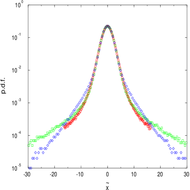
Figure 8: The rescaled probability distribution function $P(\Delta J(t)/\tilde{\sigma})$ after $N=4\times 10^{6}$ iterations, for $A=6.9115$ and $t_{1}=10^{2}$ (circles), $t_{2}=10^{3}$ (squares), $t_{4}=10^{4}$ (diamonds) with $\tilde{\sigma}(t)=\exp\{<\ln|\Delta J_{t}|>\}$.

A further natural question to be addressed is how generic is the strong anomalous behavior observed for $A=6.9115$ in the standard map. To inquire this point we have studied the diffusion properties for $(a),\,\,A=6.8115$, $(b)\,\,A=7.0115$ and $(c)\,\,A=6.4717$.

The rationale of $(a)$ and $(b)$ is to check the stability of the result (38) with respect to small changes of $A$. In the case $(a)$ strong anomalous diffusion is observed. The behavior of the moments practically coincides with that one observed for $A=6.9115$. For $(b)\,\,A=7.0115$ we observe normal diffusion: the fact has to be related to the destabilisation of the pair $(3,\pm 3)$. Finally $(c)$ corresponds to the coexistence with $(1,1)$ of two other stable islands now generated by the pair of period five accelerator modes $(5,\pm 5)$. Also in this case there is fair evidence of strong anomalous diffusion although now the crossover region between the two regimes is more extended.

At the end of this subsection we briefly discuss some results recently obtained in [42, 43] where the transport in $2-d$ symplectic maps (practically a modification of the standard map) is considered. The authors find that the anomalous diffusion is rather rare. This is particularly clear in Figs.  $5$ and $6$ of [42] where the exponent $\nu(2)$ for the kicked Harper map is shown to be always equal to $1/2$ apart very narrow regions in the control parameter space.

3.3 Anomalous diffusion in $1$-d intermittent maps

Strong anomalous diffusion may also occur in simpler dynamical systems of the form

$$\left\{\begin{array}[]{ccc}x_{t+1}&=&f(x_{t})\\ y_{t+1}&=&y_{t}+x_{t}\end{array}\right.$$ (39)

where $f(x)$ is a symmetrical Lorenz type map on the interval $[-1,1]$. Diffusion may then appear in the variable $y_{t}$. As an example we reconsidered a map previously studied by Pikovsky [26]. The function $f(x)$ is implicitly specified, $\forall z>1$, for $x\in]0,1]$ by

$$x=\left\{\begin{array}[]{ccc}\frac{1}{2\,z}[1+f(x)]^{z}&\hbox{for}&0<x<\frac{1}{2\,z}\\ f(x)+\frac{1}{2\,z}[1-f(x)]^{z}&\hbox{for}&\frac{1}{2\,z}<x<1\end{array}\right.$$ (40)

with the further requirement of monotonicity. The extension to the interval $[-1,0[$ is obtained by imposing

$$f(-x)=-f(x)$$ (41)

The resulting shape of $f(x)$ is plotted in Fig. 9.

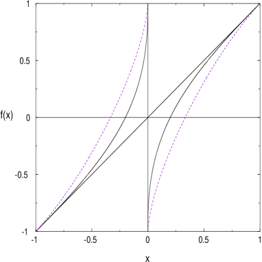
Figure 9: $f(x)$ vs $x$ from Eq. (42) for $z=2.5$ (full line) and $1.5$ (dashed line).

Thank to the implicit definition (40), by a straightforward computation, it is easy to verify that the map has a uniform density invariant distribution.

As discussed in Sec. 2 anomalous diffusion follows from power-law behavior of the correlation function of the increments of the diffusing variable. Here the latter property stems from the intermittency of the dynamics. The mapping (40) induces in the interval $[-1,1]$ two qualitatively different regions. It is not restrictive to focus on $[0,1]$

In the neighbourhood of $x=1$ the orbits perform laminar motions. The basic features of the dynamics are captured [8] by the polynomial behavior around the unstable fixed point.

$$f(x)=x+\frac{(1-x)^{z}}{2\,z}+o((1-x)^{z})$$ (42)

¿From (42) it follows that the typical duration of the laminar phase for an orbit starting from $x\approx 1$ is $T_{x}\sim(1-x)^{-(z-1)}$. Since the invariant measure is uniform a reasonable inference [40] is that the probability distribution of having laminar motion of duration $t$ scales as

$$P_{lam}(t)\sim t^{-\frac{1}{z-1}}.$$ (43)

A qualitatively different picture comes from the set $[0,\frac{1}{2\,z}]$. There the mapping has the explicit representation:

$$f(x)=[(2\,z\,|x|)^{\frac{1}{z}}-1].$$ (44)

In this second region the motion is chaotic and the increments $\Delta x_{t}=x_{t+1}-x_{t}$ decorrelate after few steps. The coexistence of the two regimes prevents the dynamics from having a typical timescale so that the increments correlation function obeys to a power law

$$C(\tau)=<\Delta x_{t+\tau}\;\Delta x_{t}>\sim P_{lam}(t)\sim t^{-1/(z-1)}$$ (45)

as it has been shown in [41]. Anomalous diffusion is therefore expected for $z>2$.

We studied the diffusion behavior of the dynamics for four values of $z$.

For $z=1.5$ the integral of the correlation (45) is convergent therefore the second moment grows linearly with time. We observe standard scaling for all the moments of power $q<3$ as shown in Fig. 10.

Figure 10: The measured scaling exponents $q\,\nu(q)$’s of the moments of the displacement $\Delta x_{t}$, as a function of the order $q$ for $z=1.5$. The dashed line $0.5\;q$ while the dotted line corresponds to $q-1.50$.

Let us note that in this case, since $\nu(2)=1/2$, the diffusion seems to be standard. Actually, because of the nonlinear behavior of $q\,\nu(q)$, one can say that this is an example of strong anomalous diffusion.

For $z=2$ the mapping coincides with (44) in all the interval $[0,1]$. This allows the use of a faster iteration algorithm. The value $z=2$ is also critical for the appearance of anomalous diffusion, in the sense $\nu(2)>1/2$, due to the divergence of $\sum_{\tau=1}^{\infty}C(\tau)$. Actually the plot of the diffusion exponent $q\,\nu(q)$ versus $q$ gives a fair evidence for strong anomalous diffusion. In Fig. 11 the moments larger than the fourth are in agreement with a ballistic dynamics $q\,\nu(q)\simeq q-0.54$ while for moments with $q<2$ it results $q\,\nu(q)\simeq 0.61\,q$.

Figure 11: The same as in Fig. 10 for $z=2.0$. The dashed line corresponds to $0.61q$ while the dotted line corresponds to $q-1.03$.

The non Gaussian behavior of the core of the probability distribution function appears also from the direct inspection of the distribution as shown in Fig. 12 where the probability distributions functions calculated for different times and rescaled by $\tilde{\sigma}$ are compared with the normal distribution.

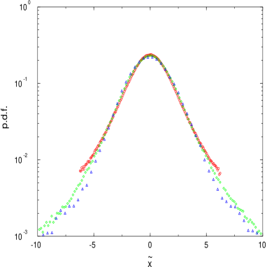
Figure 12: The rescaled probability density as in Fig. 8 but for the Pikovsky map when $z=2$ in Eq. (39).

In Fig. 13 and 14 $q\,\nu(q)$ versus $q$ is reported for $z=2.5$ and $z=3.0$.

Figure 13: The same as Fig. 10 but for $z=2.5$. The dashed line corresponds to $0.73q$ while the dotted line corresponds to $q-0.54$.

Figure 14: The same as Fig. 10 but for $z=3.0$. The dashed line corresponds to $0.78q$ while the dotted line corresponds to $q-0.44$.

As in [26] we can infer from the previous analysis the following form of the PDF of the diffusing variable $y_{t}$ for $z\geq 2$:

$$P(y,t)=[1-P_{lam}(t)]t^{-\nu_{core}}\,F_{core}(J\,t^{-\nu_{core}})+P_{lam}(t)[\delta(y-t)+\delta(y+t)].$$ (46)

A consequence of (46) is

$$q\,\nu(q)=\left\{\begin{array}[]{cc}q\,\nu_{core}&q<2\\ q-1/(z-1)&q>2\end{array}\right.$$ (47)

The predictions of (47) are in qualitative agreement with the numerical experiments. For $z<2$ the core of the probability distribution functions becomes Gaussian.

4 Conjectures and remarks

We have given rather clear numerical evidence of the presence of strong anomalous diffusion generated by nontrivial dynamics. Let us do some remarks and conjectures. As first we note (Sec. 3) that the anomalous diffusion is, in some sense, rare. For example in the flow mimicking the Rayleigh-Bénard convection (Sec. 3.1) the anomalous diffusion occurs only for some precise values of the parameter $\omega$. Something similar, even if in a weaker way, happens for the standard map (Sec. 3.2) or other $2$-d symplectic maps [42, 43]. Even though for the $1$-d intermittent maps anomalous diffusion could seem a generic feature this is not the case. Actually the origin of the superdiffusion is in the very peculiar property (marginal instability) of the fixed point (see Eq. (42)) destroyed by any generic modifications of the map. Asymptotic anomalous diffusion, at least that one generated by non ad hoc dynamical systems, seems to be a nongeneric property i.e. it disappears as soon as a small perturbation ${\cal}O(\epsilon)$ in the evolution law is introduced. However transient anomalous diffusion appears in the perturbed system up to a crossover time $t_{*}\sim\epsilon^{-\alpha}$ while for larger time standard diffusion takes place with a rather large diffusion coefficient. Therefore one can say that, even if asymptotic anomalous diffusion is very rare, its ghost is visible [35].

In all the cases here considered strong anomalous diffusion has been found to correspond to a rather simple shape of the $\nu(q)$:

$$q\,\nu(q)\simeq\left\{\begin{array}[]{ll}\nu_{1}\;q&q<q_{c}\\ q-c&q>q_{c}.\end{array}\right.$$ (48)

The above behavior suggests the existence of two different mechanisms in the diffusion process. The typical (i.e. non rare) events obey a (weak) anomalous diffusion process characterized by the exponent $\nu_{1}$, i.e. the characteristic time $\tau(l)$ at the scale $l$ behaves like $\tau(l)\sim l^{1/\nu_{1}}$, but the large deviations are essentially associated to a ballistic transport $\tau(l)\sim l$. In the flow mimicking the Rayleigh-Bénard convection the ballistic mechanism is due to the synchronization between the circulation in the cells and their oscillations. In the standard map it arises from the accelerator modes while in the $1$-d intermittent maps is due to the marginally unstable fixed point.

We do not claim of course that the above shape (48) is universal. It is rather easy, in fact, to build up a toy system for which $\nu(q)$ can be any function with the only constraint that $q\,\nu(q)$ is a convex function. Following Elliott et al. [44] we consider the velocity field

$${\mbox{\boldmath$u$}}=(u(y),w)$$ (49)

where $w$ is a constant and $u(y)$ is a given quenched random field. Neglecting the molecular diffusion the Lagrangian evolution is governed by the following equations :

$$\left\{\begin{array}[]{l}\dot{x}=u(y)\\ \dot{y}=w.\end{array}\right.$$ (50)

Now, taking for the sake of simplicity $w=1$, and $y(0)=0$ the following equation holds

$$x(t)-x(0)=\int_{0}^{t}dt^{\prime}\;u(t^{\prime})$$ (51)

which trivially relates the Lagrangian and the Eulerian statistical properties of the system. Thus, from Eq. (51) it is not difficult understand that adopting a suitable multiaffine process [45, 46] for $u(y)$ one can find the relation defining strong anomalous diffusion

$$\langle\mid x(t)-x(0)\mid^{q}\rangle\sim t^{q\,\nu(q)}\;\;\;\;\nu(q)\neq cost\;\;\;\nu(2)>\frac{1}{2}$$ (52)

with any proper shape for $\nu(q)$. A fast and efficient algorithm to generate a multiaffine process is done in [47].

A very interesting open problem is the determination of the effective diffusion equation both at long times and large scales for a system with strong anomalous diffusion. We stress the fact that if $\nu(q)\neq const$ the probability distribution $P(\Delta x,t)$ cannot obey a simple generalization of the standard diffusion equation. For sure a $P(\Delta x,t)$ corresponding to a $\nu(q)$ such that (52) holds cannot be obtained from generalized linear diffusion equation involving fractional spatial derivative as Eq. (25). Even other recently proposed linear diffusion equations with fractional derivatives both in space and in time are not able to produce such nontrivial behavior [27].

References

- [1] H.K. Moffatt, Rep. Prog. Phys., 46 (1983), 621.
- [2] J.P. Bouchaud and A. Georges, Phys. Rep., 195 (1990), 127.
- [3] A. Crisanti, M. Falcioni, G. Paladin and A. Vulpiani, La Rivista del Nuovo Cimento, 14 (1991), n.12, 1.
- [4] Ya.G. Sinai, Theor. Prob. Appl., 27 (1982), 247.
- [5] T. Geisel, J. Nierwetberg and A. Zachert, Phys. Rev. Lett., 54 (1985), 616.
- [6] R. Ishizaki, T. Horita, T. Kobayashi and H. Mori, Progr. of Theor. Phys., 85 (1991), 1013.
- [7] G.M. Zaslavsky, D. Stevens, and H. Weitzener, Phys. Rev. E, 48 (1993), 1683.
- [8] G. Matheron and G. De Marsily, Water Resouces Res., 16 (1980), 901.
- [9] G. Zumofen, J. Klafter and A. Blumen, Phys. Rev. A, 42 (1990), 4601.
- [10] M. Avellaneda and A. Majda, J. Stat. Phys., 69 (1992), 385.
- [11] T.H. Solomon, E.R. Weeks and H.L. Swinney, Physica D, 76 (1994), 70.
- [12] J.H. Misguich, J.-D. Reuss, Y.Elskens and R. Balescu, Chaos, 8 (1998), 248.
- [13] G. Zimbardo, P. Veltri, G. Basile and S. Principato, Physics of Plasmas, 7 (1995), 2653.
- [14] E. Montroll and M. Schlesinger, in Studies in Statistical Mechanics, edited by E.W. Montroll and J.L.lebowitz vol. 11, p.1, North-Holland, Amsterdam, 1984.
- [15] G.I. Taylor, Proc. Lond. Math. Soc. Ser. 2, 20 (1921), 196.
- [16] M.F. Schlesinger, B. West and J. Klafter, Phys. Rev. Lett., 58 (1987), 1100.
- [17] M. Avellaneda and A. Majda, Commun. Math. Phys., 138 (1991), 339.
- [18] M. Avellaneda and M. Vergassola, Phys. Rev. E, 52 (1995), 3249.
- [19] Ya.B. Zeldovich, Sov. Phys. Dokl., 27 (1982), 10.
-
[20]
G.I. Taylor,
Proc. R. Soc. A, 219 (1953), 186;
Proc. R. Soc. A, 225 (1954), 473 - [21] R.H. Kraichnan, Phys. Rev. Lett., 52 (1994), 1016
- [22] D. Bernard, K. Gawȩdzki, and A. Kupiainen, J. Stat. Phys., 90 (1998), 519
- [23] U. Frisch, A. Mazzino, and M. Vergassola, Phys. Rev. Lett., 80 (1998), 5532
- [24] J.-P. Bouchaud, A. Georges, J. Koplik, A. Provat and S. Redner, Phys. Rev. Lett., 64 (1990), 2503.
- [25] K. Sneppen and M.H. Jensen, Phys. Rev. E, 49 (1994), 919.
- [26] A.S. Pikovsky, Phys. Rev. A 3 (1991), 3146.
-
[27]
A.I. Saichev and G. Zaslavsky,
Chaos, (1997), 753
H.C. Fogedby, Phys. Rev. Lett. 3 (1994), 2517. - [28] J.P. Gollub and T.H. Solomon, in Proceedings of the Fritz Haber International Symposium (pagina), ed. by I. Procaccia (Plenum, New York, 1988)
- [29] T.H. Solomon and J.P. Gollub, Phys. Rev. A, 38 (1988), 6280.
- [30] R.M. Clever and F.H. Busse, J. Fluid Mech., 65 (1974), 625.
- [31] A.A. Chernikov, A.I. Neishtadt, A.V. Rogal’sky and V.Z. Yakhnin, Chaos, 1 (1991), 206.
- [32] P. Castiglione, A. Crisanti, A. Mazzino, M. Vergassola and A. Vulpiani, J. Phys. A 31, (1998), 7197.
- [33] R. Benzi, A. Sutera and A. Vulpiani, J. Phys., 14 (1981), L453.
- [34] R. Benzi, G. Parisi, A. Sutera and A. Vulpiani, SIAM Journal Appl. Math., 43 (1983), 565.
- [35] L. Biferale, A. Crisanti, M. Vergassola and A. Vulpiani, Phys. Fluids, 7 (1995), 2725.
- [36] E. Ott Chaos in Dynamical systems, Cambridge University Press, Cambridge (1993).
- [37] A.J. Lichtenberg and M.A. Lieberman Physica D 3(1988), 211.
-
[38]
J.M. Greene, J. Math. Phys. 0 (1979), 1183
(also reprinted in R.S. MacKay and J.D. Meiss, Hamiltonian Dynamical Systems Adam Hilger Bristol 1987) - [39] Y.H. Ichikawa, T. Kamimura and T. Hatori Physica D, 9 (1987) 247.
- [40] Y. Pomeau and P. manneville Com. Math. Phys., 4 (1980) 149.
- [41] S. Grossmann and H. Horner, Z. Phys. B, 6 (1985) 79.
- [42] P. Leboeuf, Physica D, 16 (1998), 8.
- [43] D. Bénisti and D.F. Escande, Phys. Rev. Lett. , 0 (1998), 4871.
- [44] F.W. Elliott, Jr., D.J. Horntrop and A.J. Majda, Chaos, 7 (1997), 39.
- [45] R. Benzi, L. Biferale, A. Crisanti, G. Paladin, M. Vergassola and A. Vulpiani, Physica D, 65 (1993), 352.
- [46] A. Juneja, D.P. Lathrop, K.R. Sreenivasan and G. Stolovitzky, Phys. Rev. E, 49 (1994), 5179.
- [47] L. Biferale, G. Boffetta, A. Celani, A. Crisanti and A. Vulpiani Phys. Rev. E, 57 (1998), R6261.