Time Delay Induced Death in Coupled Limit Cycle Oscillators

Abstract

We investigate the dynamical behaviour of two limit cycle oscillators that interact with each other via time delayed coupling and find that time delay can lead to amplitude death of the oscillators even if they have the same frequency. We demonstrate that this novel regime of amplitude ”death” also exists for large collections of coupled identical oscillators and provide quantitative measures of this death region in the parameter space of coupling strength and time delay. Its implication for certain biological and physical applications is also pointed out.

PACS numbers : 05.45.+b,87.10.+e

Coupled limit cycle oscillators provide a simple but powerful mathematical model for simulating the collective behaviour of a wide variety of systems that are of interest in physics [3, 4, 5, 6, 7, 8, 9, 10, 11, 12], chemistry [13, 14] and biological sciences [15, 16]. These oscillators have also attracted some large scale numerical [17] and novel experimental efforts [18]. For weakly coupled oscillators the predominant effect is a synchronization of the frequencies of the individual oscillators to a single common frequency once the coupling strength exceeds a certain threshold, while the amplitudes remain unaffected. For stronger couplings the amplitudes also play an important role and give rise to interesting phenomena like the Bar-Eli effect [13] where all the oscillators suffer an amplitude quenching or death [8, 11]. In general there can be a wide variety of collective behaviour including partial synchronisation, phase trapping, large amplitude Hopf oscillations and even chaotic behaviour[5, 6, 7]. In recent times there have been extensive investigations of coupled oscillator systems including elegant statistical mechanics formulations in the limit of infinite number of oscillators [9, 12].

The salient features of the behaviour of a finitely large number of oscillators (usually obtained from numerical or approximate analytic means) can often be understood by analysing just two coupled oscillators. We have carried out such an analysis to investigate the effect of time delay on the interaction between two limit cycle oscillators. Time delay is ubiquitous in most physical and biological systems [19, 20, 21], arising from finite propagation speeds of signals for example, and have not been widely studied in the context of coupled limit cycle oscillator systems. Niebuhr et al [22] and Schuster and Wagner [23] who are one of the few who have carried out such an investigation, have restricted themselves to the simpler coupled phase models where the phenomenon of amplitude death does not exist. In our model equations we have retained both the phase and amplitude response of the oscillators and we find that time delay has a significant effect on the characteristics of all the major cooperative phenomena like frequency locking, phase drift and amplitude deaths. In particular our detailed numerical investigations show that in the presence of time delay the parameter regime of amplitude death can extend down to the region of zero frequency mismatch between the oscillators. This is in sharp contrast to the situation with no time delay where all previous numerical and analytical studies [5, 7, 8, 11] show that amplitude death can occur only if the coupling between oscillators is sufficiently strong and when the frequencies are sufficiently disparate. In this Letter we confine ourselves primarily to the effect of time delayed coupling on the phenomenon of amplitude death and present a detailed numerical and analytical estimate of the parameter space in coupling strength and time delay where such a death can occur for identical oscillators. We also establish that this effect is not an artefact of the simple two oscillator model, but can occur for a system of large number of globally (or locally) coupled identical oscillators (including the continuum limit of $N\rightarrow\infty$).

We analyse the following model equations:

$$\dot{Z}_{1}(t)=(1+i\omega_{1}-\mid Z_{1}(t)\mid^{2})Z_{1}(t)$$ (1)

$$+K[Z_{2}(t-\tau)-Z_{1}(t)],$$ (2)

$$\dot{Z}_{2}(t)=(1+i\omega_{2}-\mid Z_{2}(t)\mid^{2})Z_{2}(t)$$ (3)

$$+K[Z_{1}(t-\tau)-Z_{2}(t)],$$ (4)

where $\tau$ is a measure of the time delay, $K$ is the coupling strength, $\omega_{1,2}$ are the intrinsic frequencies of the two oscillators and $Z_{1,2}$ are complex. The model is a generalization of the diffusively and linearly coupled oscillators studied extensively for example in [5, 13]. The time delay parameter is introduced in the argument of the coupling oscillator (e.g. $Z_{2}$ in (1)) to physically account for the fact that its phase and amplitude information is received by oscillator $Z_{1}$ only after a finite time $\tau$ (due to finite propagation speed effects). In the absence of coupling ($K=0$) each oscillator has a stable limit cycle at $\mid Z_{i}\mid=1$ on which it moves at its natural frequency $\omega_{i}$. The coupled equations represent the interaction between two weakly nonlinear oscillators (that are near a Hopf bifurcation) and whose coupling strength is comparable to the attraction of the limit cycles. It is important then to retain both the phase and amplitude response of the oscillators[5]. The state $Z_{i}=0$ is an equilibrium solution of the system of equations [(1) and (3)]. For $K=0$ this equilibrium state is linearly unstable since the individual oscillators tend to stable limit cycle states $\mid Z_{i}\mid=1$. The stability of amplitude death for $K\neq 0$ has been studied in great detail by Aronson et al[5] for system ((1,(3)) in the absence of any time delay in the coupling (i.e. for $\tau=0$). The conditions for stability found by them are,

$$K>1\;\;\;and\;\;\;\Delta=\mid\omega_{1}-\omega_{2}\mid>2\sqrt{2K-1},$$ (5)

which shows that amplitude death can occur in this case only for sufficiently large values of $\Delta$ provided $K>1$.

In Fig. 1(a), we reproduce the bifurcation diagram of Aronson et.al[5] where the region marked $I$ represents the amplitude death region and the dotted curves mark the boundary as defined by condition (5). The two bounding curves intersect at the point ($K=1,\Delta=2$). Regions marked ($II$) and ($III$) represent phase locked and phase drift regions respectively which we will not discuss in detail here. In Fig. 1(b) we present the bifurcation diagram of (1-3) for $\tau=0.0817$. Note that in contrast to the diagram of Fig. 1(a), the amplitude death region now extends down to $\Delta=0$ and has a finite extent along the coupling strength ($K$) axis. We find that the phenomenon persists for a range of $\tau$ after which the bifurcation curve lifts up from the $\Delta=0$ line and identical oscillators can no longer suffer death. Fig. 2(a) shows this region, for different values of $\omega$, in $\tau-K$ space for which amplitude death of identical oscillators can occur. The size of this death island is a function of the frequency of the oscillators ($\omega$), as shown by the other curves. We shall soon show that the size is also a function of $N$, the number of oscillators. The bifurcation curves (including the island boundaries) have been obtained from a linear stability analysis of (1),(3) about the origin $(Z_{1}=Z_{2}=0$) as well as direct numerical integration of the equations. Assuming the linear perturbations to vary as $e^{\lambda t}$ the

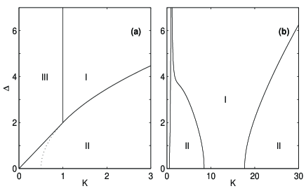
FIG. 1.: Bifurcation diagram of Eqns.(1-3). (a) $\tau=0$. Region $I$ is the amplitude death region, $II$ is the phase locked region, and $III$ corresponds to the phase drift or incoherent region. (b) $\tau=0.0817$, and $\bar{\omega}=10$. The death region extends down to $\Delta=0$ indicating that identical oscillators can suffer amplitude death. The phase locked region is split into two disjoint regions.

characteristic eigenvalue equation we get is,

$$(1-K+i\omega_{1}-\lambda)(1-K+i\omega_{2}-\lambda)-$$ (6)

$$K^{2}e^{-2\lambda\tau}=0,$$ (7)

where $\lambda$ is the complex eigenvalue and the complete set of eigenvalues includes those arising from the complex conjugate equations of (1) and (2) . Setting ${\it Real}(\lambda)=0$ in (6) and separating the real and imaginary parts, the equations for the critical curves (i.e. the marginal stability condition) are,

$$\lambda_{I}^{2}+2\lambda_{I}\bar{\omega}+\bar{\omega}^{2}-\frac{\Delta^{2}}{4}-(1-K)^{2}$$ (8)

$$+K^{2}\cos(2\lambda_{I}\tau)=0,$$ (9)

$$2(1-K)(\bar{\omega}+\lambda_{I})+K^{2}\sin(2\lambda_{I}\tau)=0.$$ (10)

where $\lambda_{I}={\it Imag}(\lambda)$ and $\bar{\omega}=(\omega_{1}+\omega_{2})/2$ is the mean frequency. Eliminating $\lambda_{I}$ between (8) and (10) and considering the full set of eigenvalues , we obtain the following transcedental relation between $K,\Delta$ and $\tau$ which is now the modified marginal stability condition in place of (5),

$$g\alpha=K^{2}\sin(\alpha\tau\pm 2\bar{\omega}\tau),$$ (11)

where $\alpha=\sqrt{\Delta^{2}-4g^{2}\mp 4\sqrt{K^{4}-g^{2}\Delta^{2}}}$, and $g=1-K$. Note that for $\tau=0$, the above relation readily simplifies to (5) and yields the marginal stability curves $K=1$ and $2K=1+\frac{\Delta^{2}}{4}$. Figure 1(b). is a numerical plot of (11) for $\tau=0.0817$.

To obtain a condition for the death of identical oscillators we repeat the analysis with $\omega_{1}=\omega_{2}=\omega$ in (6) and after eliminating $\lambda_{I}$, obtain the relations

$$\tau=\frac{\cos^{-1}(1-1/K)}{\omega-\sqrt{2K-1}}\;;\;\;\tau=\frac{\pi-\cos^{-1}(1-1/K)}{\omega+\sqrt{2K-1}}.$$ (12)

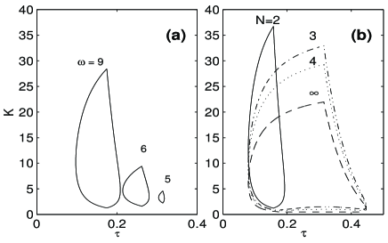
FIG. 2.: (a) The region of amplitude death for $N=2$ as a function of the common intrinsic frequency. The size of the the island decreases with decreasing frequency and vanishes below a certain threshold. (b) The death islands as a function of the number of globally coupled oscillators. Each oscillator is assumed to have an intrinsic frequency of $\omega=10$. The death island survives even in the limit of $N\rightarrow\infty$.

The region of intersection between the two curves (12) corresponds to the death island region of Fig. 2(a). It demonstrates the only stability switches (of the origin) that take place as a function of $\tau$. For a given value of $\omega$ and at a fixed $K$ we move (by varying $\tau$) from an unstable region into a stable region as we cross the left boundary of the island to emerge again into an unstable region as we cross the right boundary of the island. No other amplitude death islands are seen for larger values of $\tau$ (for a fixed $\omega$). We have also confirmed this analytically by looking at the behaviour of the supremum of the real parts of the roots of the transcedental equation, $d\lambda_{R}/d\tau$ (obtained from (4) with $\Delta=0$) as a function of $\tau$ in the various parameter regimes[20]. The detailed mathematical proof of this result will be published elsewhere.

Can this phenomenon occur for an arbitrary number of oscillators? To answer this question we have investigated the following generalized set of globally coupled equations:

$$\dot{Z}_{i}(t)=(1+i\omega_{i}-\mid Z_{i}(t)\mid^{2})Z_{i}(t)+$$ (13)

$$\frac{2K}{N}\sum_{j=1}^{N}[Z_{j}(t-\tau)-Z_{i}(t)]-$$ (14)

$$\frac{2K}{N}[Z_{i}(t-\tau)-Z_{i}(t)],$$ (15)

where $i=1,....,N$ and the last term on the right hand side has been included to remove the self-coupling term. For $\tau=0$, (13) reduces to the set of equations that have been extensively studied by Ermentrout [11], Mirollo and Strogatz [8], and others[6]. Mirollo and Strogatz[8] have provided rigorous analytical and numerical conditions for amplitude death in such a system. Their conclusions, in general, are similar to the case of $N=2$, namely, that one needs a sufficiently large variance in frequencies for death to occur and $K$ has to be sufficiently large. We have been able to carry out a similar linear stability analysis of (13) around the origin for the case of finite $\tau$ and for a large number of identical oscillators ($\omega_{j}=\omega,\;\;\;j=1,...,N$). The resulting stability condition yields the following bounding curves for the death island region:

$$\tau=\frac{\cos^{-1}p}{\omega-\sqrt{4Kb-1}}\;;\;\;\tau=\frac{2\pi-\cos^{-1}p}{\omega+\sqrt{4Kb-1}},$$ (16)

$$\tau=\frac{\cos^{-1}(\frac{b}{b-1}p)}{\omega+\sqrt{q}}\;;\;\;\tau=\frac{2\pi-\cos^{-1}(\frac{b}{b-1}p)}{\omega-\sqrt{q}},$$ (17)

where $p=1-1/(2Kb)$, $q=4K^{2}-1+4Kb(1-2K)$ and the factor $b=(1-1/N)$ introduces the $N$ dependence of the island size explicitly. In Fig. 2(b) we have plotted these islands for $N=2,3,4$ and $N=\infty$. To confirm these results we have also numerically scanned the region with a direct numerical integration of (13) for a large number of oscillators, upto $N=10000$, and found excellent agreement. We have also carried out a similar study for a large number of locally coupled identical oscillators (nearest neighbour coupling [4]) with periodic boundaries and find that time delay introduces death islands in such systems as well. Thus it appears that in the presence of finite time delay in the mutual coupling, amplitude death of identical oscillators is a fairly universal phenomenon and occurs for any arbitrary number $N$ of oscillators extending upto $N=\infty$ over a range of $\tau$ and $K$ values. To the best of our knowledge such a result has not been realised in the past and may have important applications in biological or physical systems. There are many physical examples of amplitude death in real systems. One of the earliest that was investigated both theoretically and experimentally is that of coupled chemical oscillator systems e.g. coupled Belousov-Zhabotinskii reactions carried out in coupled stirred tank reactors[13, 14]. They can also occur in ecological contexts where one can imagine two sites each having the same predator-prey mechanism which causes the number density of the species to oscillate. If the species are capable of moving from site to site at a proper rate (appropriate coupling strength) the two sites may become stable (stop oscillating) and acquire constant populations. Another important application of this concept is in pathologies of biological oscillator networks e.g. an assembly of cardiac pacemaker cells[15]. Amplitude death signifies cessation of rhythmicity in such a system which is otherwise normally spontaneously rhythmic for other choices of parameters. For the onset of such an arrhythmia, current models based on coupled oscillator networks need to assume a significant spread in the natural frequencies of the constituent cells (oscillators)[8]. Our work demonstrates that this assumption may not be necessary if one takes into account time delay effects arising naturally from the finite propagation times of the signals exchanged between the cells. Another possible application is in the area of high power microwave sources where it is proposed to enhance the microwave power production by phase locking a large number of sources such as relativistic magnetrons[24]. Time delay effects, arising from the finite propagation time of information signals traveling through the connecting waveguide bridges, could impose important limitations on the connector lengths and geometries in these schemes. Our findings could provide a guideline in this direction. It should be noted that a form of oscillator death described in [25] for identical oscillators is not a genuine amplitude death since it occurs in the context of a phase only model. Time delay in our study provides a new mechanism for genuine amplitude death to occur in coupled identical oscillators.

Finally, it is worthwhile to mention that time delay can introduce other interesting phenomena as well, some of which have been studied in the context of the phase only model and need to be investigated for the more general phase and amplitude model. Our numerical results, for

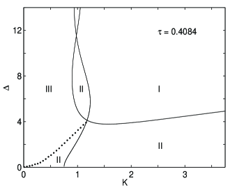
FIG. 3.: The bifurcation diagram of Eqs. (1) and (3) for $\tau=0.4084$ and $\bar{\omega}=10$. The amplitude death region (I) is surrounded by the phase locked regions (II). The dotted curve which separates the incoherent (III) and the phase locked regions is obtained from numerical integration of the original equations.

example, show that the bifurcation diagram of the system in the presence of time delay has a significantly richer structure. Fig. 3 is an example for the $N=2$ system for $\tau=0.4084$, which can be contrasted with the Aronson et al[5] diagram of Fig. 1(a). Note that one no longer has the clean separation of the Bar-Eli region, the phase locked region and the phase drift region into three disjoint regions that converge at a single degenerate point. Instead the phase locked region now always surrounds the Bar-Eli region and the single degenerate point is replaced by a series of $X$ points resulting from the braided structure of the phase locked region in the vertical direction. At large values of $K$ other bifurcation curves appear in the phase locked region indicating the appearance of higher frequency states [23]. A detailed investigation of various properties of this rich phase diagram, including stability studies of the various states, is now in progress and will be reported elsewhere.

REFERENCES

- [1] Email address: tapovan@plasma.ernet.in
- [2] Permanent address: 12 Billings St., Acton, MA 01720.
- [3] A.K. Jain, K.K. Likharev, J.E. Lukens and J.E. Sauvageau, Phys. Rep. 109, 309 (1984);D.S. Fisher, Phys. Rev. B 31, 1396 (1985); P. Hadley, M. R. Beasley and K. Wiesenfeld, Phys. Rev. B 38, 8712 (1988); Appl. Phys. Lett. 52, 1619 (1988).
- [4] S. H. Strogatz, R. E. Mirollo, J. Phys. A.:Math. Gen. 21, L699 (1988); S. H. Strogatz, R. E. Mirollo, Physica (Amsterdam) 31D, 143 (1988).
- [5] D.G. Aronson, G.B. Ermentrout and N. Koppel, Physica (Amsterdam) 41D, 403 (1990).
- [6] Y. Aizawa, Prog. Theor. Phys. 56, 703 (1976); M. Shiino and M. Frankowicz, Phys. Lett. A 136, 103 (1989).
- [7] P. C. Matthews and S. H. Strogatz, Phys. Rev. Lett. 65, 1701 (1990); P. C. Matthews, R. E. Mirollo, and S. H. Strogatz, Physica (Amsterdam) 52D, 293 (1991); N. Nakagawa and Y. Kuramoto, Physica (Amsterdam) D75, 74 (1994).
- [8] R. E. Mirollo and S. H. Strogatz, J. Stat. Phys. 60, (1990) 245-262.
- [9] Y. Kuramoto, Prog. Theor. Phys. Suppl. No.79, 223-240 (1984); Y. Kuramoto and I. Nishikawa, J. Stat. Phys. 49, 569 (1987).
- [10] J. W. Swift, S. H. Strogatz, and K. Wiesenfeld, Physica (Amsterdam) 55D, 239 (1992).
- [11] G. B. Ermentrout, Physica (Amsterdam) 41D, 219 (1990).
- [12] H. Daido, J. Stat. Phys. 60, 753 (1990); H. Daido, Physica (Amsterdam) 91D, 24 (1996) and references there in; H. Daido, Phys. Rev. Lett. 78, 1683 (1997).
- [13] K. Bar-Eli, Physica (Amsterdam) 14D, 242 (1985).
- [14] Michael F. Crowley and Irving R. Epstein, J. Phys. Chem. 93, 2496 (1989).
- [15] A. T. Winfree, The Geometry of Biological Time (Springer-Verlag, New York, 1980); The Three-Dimensional Dynamics of Electrochemical Waves and Cardiac Arrythmias (Princeton University Press, Princeton, NJ, 1987).
- [16] Mitsuo Kawato and Ryoji Suzuki, J. theor. Biol. 86, 547 (1980).
- [17] Kazuhiro Satoh, J. Phys. Soc. Japan 58, 2010 (1989).
- [18] A. A. Brailove and P. S. Linsay, Int. J. Bifurcation Chaos 6, 1211 (1996).
- [19] L. Glass and M. C. Mackey, Science 197, 287 (1977).
- [20] K. L. Cooke and Z. Grossman, J. Math. Anal. App. 86, 592 (1982); F. G. Boese, J. Math. Anal. App. 140, 510 (1989).
- [21] J. K. Hale and N. Sternberg, J. Comp. Phys. 77, 221 (1988); W. Wischert, et. al., Phys. Rev. E 49, 203 (1994).
- [22] E. Niebur, H.G. Schuster and D. Kammen, Phys. Rev. Lett. 67, 2753 (1991).
- [23] H.G. Schuster and P. Wagner, Prog. Theor. Phys. 81, 939 (1989).
- [24] J. Benford, H. Sze, W. Woo, R.R. Smith and B. Harteneck, Phys. Rev. Letts. 62, 969 (1989).
- [25] G.B. Ermentrout and N. Kopell, SIAM J. App. Math 50, 125 (1990).